2602.15547

# jina-embeddings-v5-text: Task-Targeted Embedding Distillation **Authors**: - xxx, xxx (Jina AI GmbH, Prinzessinnenstraße 19–20, 10969 Berlin, Germany) - Jina by Elastic (2024/02/26) Abstract Text embedding models are widely used for semantic similarity tasks, including information retrieval, clustering, and classification. General-purpose models are typically trained with single- or multi-stage processes using contrastive loss functions. We introduce a novel training regimen that combines model distillation techniques with task-specific contrastive loss to produce compact, high-performance embedding models. Our findings suggest that this approach is more effective for training small models than purely contrastive or distillation-based training paradigms alone. Benchmark scores for the resulting models, jina-embeddings-v5-text-small and jina-embeddings-v5-text-nano, exceed or match the state-of-the-art for models of similar size. jina-embeddings-v5-text models additionally support long texts (up to 32k tokens) in many languages, and generate embeddings that remain robust under truncation and binary quantization. Model weights are publicly available, hopefully inspiring further advances in embedding model development. footnotetext: Equal contribution. 1 Introduction Information retrieval (IR) systems increasingly rely on text embedding models as first-stage retrievers, replacing or augmenting traditional methods. These models map queries and documents into a shared dense vector space, enabling efficient retrieval via nearest-neighbor search. These dense embeddings see use in a wide array of IR applications, including web search, question-answering, and retrieval-augmented generation, as well as other purposes like recommendation systems, clustering, classification and quantification of semantic similarity. The prevailing architecture for embedding models is a transformer architecture augmented with a pooling layer, first introduced for Sentence-BERT Reimers and Gurevych (2019). Recent models, like Qwen3Embeddings Zhang et al. (2025b) and Embedding-Gemma Vera et al. (2025), are trained using contrastive learning. Alternatively, knowledge distillation provides an efficient mechanism for training small models to mimic the behavior of one or more teacher models, as exemplified by the Jasper model Zhang et al. (2024a). This work combines model distillation with task-specific contrastive loss training, demonstrating that (1) distillation outperforms naive contrastive training, (2) our combined approach leads to further improvements compared to a pure distillation-based approach, and (3) the resulting models perform on the MTEB benchmarks Enevoldsen et al. on-par with or better than recent models with comparable sizes. Specifically, this work’s contributions are: - Training Method: We introduce a new training method that combines distillation with task-specific, specialized training objectives - Empirical Analysis of Distillation Methods: We present a comparative analysis of different distillation methods for embedding models. - Model Release: We have released the resulting model weights to the public https://huggingface.co/collections/jinaai/jina-embeddings-v5-text in order to foster advances in the field. 2 Related Work Related work spans work about distilling language models in general, research into distillation specifically for embedding models, and contrastive multi-task learning. 2.1 Language Model Distillation Model distillation is an approach to creating compact language models that has been used to create models like DistilBERT Sanh et al. (2019). Distillation uses specialized loss functions to align a “student” model with a “teacher.” For DistilBERT, this means one function to align their outputs, and one to align the hidden layers using cosine loss. Alternatively, MiniLM models Wang et al. (2020) are distilled by mimicking the self-attention behavior of the parent model. TinyBERT Jiao et al. (2020) uses a pre-trained version of BERT during pre-training and a fine-tuned version for fine-tuning. Chen et al. (2021) follow up on this work by developing a reranker model using the same technique with additional labeled data. 2.2 Embedding Model Distillation Early approaches Hofstätter et al. (2020); Menon et al. (2022) to the distillation of embedding models focused on aligning new models with the similarity scores of teacher models. Kim et al. (2023) employ a projection layer to align teacher and student embedding spaces and perform distillation on the embeddings directly. Yang et al. (2024); Musacchio et al. (2025) train cross-lingual dense retrieval models using machine translation. Zhang et al. (2024a) introduce techniques for multi-teacher distillation, using both embedding alignment and score-based distillation methods, applied over multiple training stages. Formont et al. add a Gaussian kernel-based loss component for multi-teacher distillation. This appears to improve performance for embedding-based distillation with a projection layer setup. Also, Zhang et al. (2025a) recently proposed an approach that consists of a distillation and a contrastive training stage. Unlike our method, it only fine-tunes an existing embedding model and does not address differences in optimization methods for different task types. 2.3 Task-Specific Embedding Training Researchers have also proposed a variety of techniques to train embedding models to jointly optimize for different tasks and thereby resolve task conflicts. Joint optimization to support multiple target domains commonly involves combinations of loss functions Wang et al. (2014); Chen et al. (2024) or varying the training objective during training Mohr et al. (2024). Additionally, generating multiple models via task-specific fine-tuning and then merging their weights using “model soup” methods has proven productive Vera et al. (2025). Instruction tuning has been proposed to resolve task conflicts in both text Su et al. (2023) and image Zhang et al. (2024b) retrieval models. Instructions enable fine-grained manual adjustments to improve embedding performance for specific domains and task types. However, achieving strong performance with hand-crafted instructions requires additional labeling effort from practitioners. Alternatively, LoRA adapters allow task-specific adaptations to be trained independently and have also been shown to resolve task conflicts effectively Sturua et al. (2025). 3 Model Architecture <details> <summary>img/architecture.png Details</summary>  ### Visual Description \n ## Diagram: Transformer Model with LoRA Adapters ### Overview This diagram illustrates the architecture of a Transformer model augmented with Task-Specific LoRA (Low-Rank Adaptation) adapters. The diagram shows the flow of data from model inputs, through the Transformer model, to an embedding vector, and highlights the role of LoRA adapters in tailoring the model for specific tasks. ### Components/Axes The diagram consists of the following components: * **Model Inputs:** Labeled "Model Inputs" at the bottom. * **Transformer Model:** A large teal-colored rectangle labeled "Transformer Model". * **Task-Specific LoRA Adapters:** Three teal-colored boxes labeled "[RETRIEVAL]", "[CLUSTERING]", and "[TEXT MATCHING]". An ellipsis (...) indicates that there are more adapters. * **Last Token Pooling:** A rectangular box labeled "Last Token Pooling". * **Embedding Vector:** A rectangular box labeled "Embedding Vector". * **Input Text:** A text label within the "Model Inputs" section, reading "Input Text". * **prompt_name:** A text label within the "Model Inputs" section, reading "prompt_name = document". * **task:** A text label within the "Model Inputs" section, reading "task = text-matching". * **truncate_dim:** A text label on the left side, reading "truncate_dim = 512". * **Embedding Vector Values:** Three values displayed within the "Embedding Vector" box: 8.31, -0.17, and 1.95. * **Arrow with Length Indicator:** An arrow pointing from the "Embedding Vector" box, with a yellow line indicating a length and associated values. ### Detailed Analysis or Content Details The diagram shows a data flow starting from "Model Inputs". 1. **Model Inputs:** The inputs consist of "Input Text", a "prompt_name" set to "document", and a "task" set to "text-matching". A "truncate_dim" parameter is set to 512. 2. **Transformer Model:** The "Input Text" and other inputs are fed into the "Transformer Model". 3. **Task-Specific LoRA Adapters:** The output of the "Transformer Model" is then passed through one of several "Task-Specific LoRA Adapters". The diagram shows three adapters: "[RETRIEVAL]", "[CLUSTERING]", and "[TEXT MATCHING]". The ellipsis suggests there are more adapters available. 4. **Last Token Pooling:** The output of the LoRA adapters is then passed to "Last Token Pooling". 5. **Embedding Vector:** The output of "Last Token Pooling" is an "Embedding Vector". The vector contains three values: 8.31, -0.17, and 1.95. 6. **Feedback Loop:** A feedback loop is shown on the left side of the diagram, connecting the "Embedding Vector" back to the "Transformer Model". An arrow indicates a length, with values associated with it. The Embedding Vector values are: * 8.31 * -0.17 * 1.95 ### Key Observations The diagram highlights the modularity of the Transformer model through the use of LoRA adapters. This allows the same base Transformer model to be adapted for different tasks without retraining the entire model. The feedback loop suggests a potential iterative refinement process. The values within the embedding vector are numerical representations of the input data after processing. ### Interpretation The diagram demonstrates a technique for efficiently adapting large language models (LLMs) to specific tasks. LoRA adapters provide a lightweight mechanism for task specialization, reducing the computational cost and data requirements compared to full fine-tuning. The "truncate_dim" parameter suggests that the input text is being truncated to a maximum length of 512 tokens. The embedding vector represents a condensed, numerical representation of the input text, capturing its semantic meaning. The feedback loop could represent a mechanism for refining the embedding based on the task-specific adapter's output. The diagram suggests a system designed for flexibility and efficiency in applying a powerful Transformer model to a variety of downstream tasks. 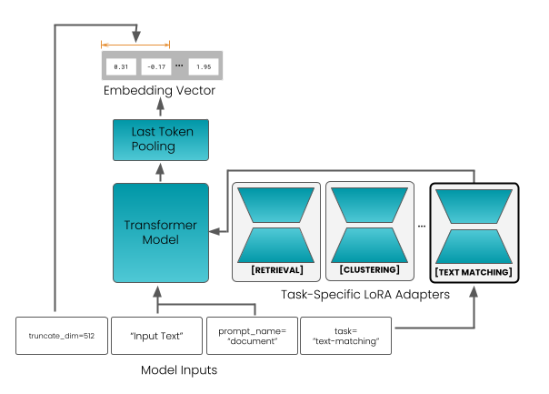</details> Figure 1: Architecture of jina-embeddings-v5-text. Table 1: Attributes of the Base Models and the Resulting Embedding Models | Model | Parameters | RoPE | Max. | Emb. | | | --- | --- | --- | --- | --- | --- | | Name | Base | LoRA | $\bm{\theta}$ | Tokens | Dim. | | j-v5-text-small | 596M | 4 $×{}$ 20.2M | 3.5M | 32K | 1024 | | j-v5-text-nano | 212M | 4 $×{}$ 6.7M | 1M | 32K | 768 | | Base Models | | | | | | | Qwen3-0.6B | 600M | – | 1M | 32K | 1024 | | EuroBERT-210M | 210M | – | 250K | 8K | 768 | Figure 1 displays the model architecture. It is a transformer model that closely follows the schema of other pre-trained language models Boizard et al. (2025); Yang et al. (2025). The model translates a text input into a single embedding via last-token pooling, i.e., it uses the embedding of the end-of-sequence token produced by the transformer layers. Following the approach of Sturua et al. (2025), the model includes LoRA adapters to support multiple tasks that are difficult to optimize for jointly. These tasks are: retrieval, semantic similarity, clustering, and classification. Adapters are loaded together with the model weights, and users select the appropriate one at inference time. To support asymmetric retrieval, jina-embeddings-v5-text distinguishes between query and document inputs by pre-pending a prefix to the input text – either "Query:" or "Document:". Other tasks use a single "Document:" prefix. Embeddings can also be truncated for downstream efficiency, enabled by using Matryoshka Representation Learning during training Kusupati et al. (2022). Table 1 summarizes the attributes of both embedding models and their underlying backbone models. 4 Training For training our embedding models we use the pre-trained language models EuroBERT-210m Boizard et al. (2025) for jina-embeddings-v5-text-nano and Qwen3-0.6B-Base Yang et al. (2025) for jina-embeddings-v5-text-small (see Table 1). Both models are multilingual. EuroBERT’s training focuses on 15 major European and global languages: English, French, German, Spanish, Chinese, Italian, Russian, Polish, Portuguese, Japanese, Vietnamese, Dutch, Arabic, Turkish, and Hindi. It also includes some materials in other languages. Qwen3-0.6B-Base lists 119 languages: https://qwen.ai/blog?id=qwen3 (Last Access: 01/27/2026). Our training method consists of two main stages: Embedding Distillation: We use distillation to transfer knowledge from Qwen3-Embedding-4B model https://huggingface.co/Qwen/Qwen3-Embedding-4B (Last Access: 01/27/2026), a much larger, trained embedding model Zhang et al. (2025b). The goal is to enable a small model to approximate the performance of the larger model without requiring instruction-style prompts or other prompt engineering for embedding generation. Task-Specific Adapter Training: In this stage, we freeze the model weights and train LoRA adapters for better performance in broad task categories: retrieval, semantic similarity, clustering, and classification. 4.1 First-Stage: Embedding Distillation Distillation requires a “student” model, a “teacher” model, and training data for both to process. Our training data consists of text pairs $(q,d)$ that consist of a text that functions as a query $q$ and one that functions as a document to retrieve $d$ , e.g., title-abstract and question-answer pairs. The Qwen3 teacher model has been trained to follow instructions when generating embeddings, enabling users to provide relevant extra-textual information, like whether an embedding is to be used as a query or a document, or domain-relevant information like that a text is a scientific abstract or encyclopedia entry. This enables the model to position the embedding better in its semantic space and improves task performance. However, it leads to ambiguity when we do not know what instructions are empirically most useful and makes it harder for us to transfer knowledge through distillation. Therefore, we make only minimal use of instructions during distillation. For the student, we only provide generic query/document prefixes (described in Section 4.2.1), and for the teacher, the general instruction: “Given a web search query, retrieve relevant passages that answer the query”, which is provided as a default in its sentence transformer configuration. https://huggingface.co/Qwen/Qwen3-Embedding-4B/blob/main/config_sentence_transformers.json (Last Access: 02/13/2026) 4.1.1 Positional Information We use rotary positional embeddings (RoPE) Su et al. (2024) to inject positional information during attention calculation. This technique uses rotation matrices and a parameter $\theta$ , which controls the rotation frequencies. Using a higher $\theta$ at inference time and a lower one during training has been shown to improve performance on texts that are longer than those seen during training Zhang et al. (2024c); Liu et al. (2024). Since our training data consists of relatively short texts, but we want the models to perform well on long ones, we train with much smaller $\theta$ values, as seen in Table A1, than the ones we use at inference time, as shown in Table 1. 4.1.2 Loss Function At each training step, we apply the student/teacher model to a batch of pairs $(q,d)$ , resulting in two batches of embeddings: $$ \mathcal{B}_{S}=\{(\mathbf{x}^{S}_{i},\mathbf{y}^{S}_{i})\}_{i=1}^{B},\;\mathbf{x}^{S}_{i},\mathbf{y}^{S}_{i}\in\mathbb{R}^{n} $$ and $$ \mathcal{B}_{T}=\{(\mathbf{x}^{T}_{i},\mathbf{y}^{T}_{i})\}_{i=1}^{B},\;\mathbf{x}^{T}_{i},\mathbf{y}^{T}_{i}\in\mathbb{R}^{m} $$ The dimensionality of the teacher embeddings $m$ is higher than the dimensionality of the student embeddings $n$ . We use a linear projection layer $\psi:\mathbb{R}^{n}→\mathbb{R}^{m},\;\psi(\mathbf{z})=W\mathbf{z}+\mathbf{b}$ to project the student embeddings into the teacher’s embedding space, enabling us to use cosine similarity $\phi$ to determine similarity scores. Our distillation loss $\mathcal{L}_{\mathrm{distill}}$ is a sum of cosine distances between the two sets of embeddings: $$ \displaystyle\mathcal{L}_{\mathrm{distill}}=\sum_{i=1}^{B}\Bigg(\sum_{\mathbf{z}\in\{\mathbf{x},\mathbf{y}\}}\bigl[1-\phi\bigl(\psi(\mathbf{z}^{S}_{i}),\;\mathbf{z}^{T}_{i}\bigr)\bigr]\Bigg) \tag{1} $$ Theoretically, it is possible to project the teacher embeddings to the dimensionality of the student embeddings instead. However, we found that this is less effective, as shown in Section 5.3.2. 4.1.3 Training Procedure Distillation proceeds in two phases: General-Purpose Training: First, we performed training using a large, diverse collection of text pairs, drawn from over 300 datasets in over 30 languages. Training is conducted for 50,000 steps with the hyperparameters documented in Table A1. Long Context Training: General-purpose training for jina-embeddings-v5-text-small produced unsatisfactory performance on long documents, as shown in Table A18, and we undertook further training on that model to improve long sequence embeddings quality. This training incorporated a curated collection of materials, including synthetic documents designed to retrieve documents based on specific contents embedded in long, high-density, noisy texts. It also contained natural long texts, such as book chapters and long-form articles, paired with LLM-generated queries. This dataset includes multilingual document-query pairs with texts of 1,000 to 4096 tokens, ensuring that long document performance is robust across languages. We also lowered the $\theta$ parameter of the positional embeddings and increased the maximum sequence length. That facilitates smoother interpolation of frequencies across the extended context window, leading to better performance on long texts. Detailed hyperparameter configurations are stated in Table A1. 4.2 Second-Stage: Task-Specific Adapters We froze the weights in the distillation-trained model to train the LoRA adapters for specific tasks. For each task category, we have a separate adapter. This avoids problems with conflicting optimization objectives. In this second stage of training, we used different loss functions and training data for each adapter. We also re-used the projection layer weights trained in the first stage. 4.2.1 Asymmetric Retrieval Adapter Asymmetric retrieval is based on the insight that queries and retrieval targets are usually very different from each other. Queries are almost always much shorter than the document they’re matched to, and are often worded differently, or use different syntax, like question answering. Consequently, encoding queries and documents differently can yield large improvements in retrieval. We implement this asymmetry with prefixes, specifically by pre-pending "Query:" to inputs intended to be used as queries and "Document:" to texts intended to be retrieval targets (see Section 3). Training data for this adapter consists of triplet datasets containing queries, relevant documents, and hard negatives, as well as the long-context datasets described in Section 4.1.3. For texts in the long-context datasets, the maximum sequence length and batch size were adjusted dynamically in each training step, depending on which dataset was sampled. Detailed hyperparameter values are provided in Appendix A1. We also use a combination of three loss functions: Contrastive Loss: We use InfoNCE loss Oord et al. (2018) with hard negatives Karpukhin et al. (2020). Given a batch of size $B$ , let $X=\{\bm{x}_{i}\}_{i=1}^{B}$ denote the query embeddings and $Y=\{\bm{y}_{i}\}_{i=1}^{B}$ their corresponding relevant document embeddings. For each query embedding $\bm{x}_{i}$ , we define a negative set $\mathcal{N}_{x_{i}}$ consisting of all non-matching in-batch document embeddings and additional mined hard negatives, i.e., semantically related but incorrect documents. Based on the the temperature-scaled exponential cosine similarity $S(\bm{x},\bm{y})=\exp(\phi(\bm{x},\bm{y})/\tau)$ , the contrastive loss is defined as follows: $$ \mathcal{L}_{\text{NCE}}^{q\rightarrow d}=-\frac{1}{B}\sum_{i=1}^{B}\log\left(\frac{S(x_{i},y_{i})}{S(x_{i},y_{i})+\sum\limits_{n\in\mathcal{N}_{x_{i}}}S(x_{i},n)}\right) \tag{2} $$ where $\tau$ is a learnable temperature parameter. Distillation Loss: We retain the same knowledge distillation loss used during the first stage of training (Equation (1)), ensuring that the retrieval adapter preserves the general-purpose embedding quality established by the base model. Spread-Out Regularizer Following Vera et al. (2025), we apply a global orthogonal regularizer (GOR) (Zhang et al., 2017) that encourages embeddings to be distributed more uniformly across the embedding space, improving their expressive capacity. This also improves robustness to quantization and enables more efficient retrieval under approximate nearest neighbor (ANN) search. The GOR loss is defined as: $$ \displaystyle\mathcal{L}_{\text{GOR}}={} \displaystyle\frac{1}{B(B-1)}\sum_{\begin{subarray}{c}i,j\in\mathcal{B}\\ i\neq j\end{subarray}}(\mathbf{q}_{i}^{\top}\mathbf{q}_{j})^{2} \displaystyle+\frac{1}{B(B-1)}\sum_{\begin{subarray}{c}i,j\in\mathcal{B}\\ i\neq j\end{subarray}}(\mathbf{p}_{i}^{+\top}\mathbf{p}_{j}^{+})^{2} \tag{3} $$ where $\mathbf{q}_{i}$ and $\mathbf{p}_{i}^{+}$ denote the query and positive document embeddings, respectively. This loss penalizes high pairwise similarity between non-matching embeddings, driving them to behave as if uniformly sampled from the unit sphere. Combined Objective: The final training objective for the retrieval adapter is a linear combination of the three loss functions: $$ \mathcal{L}_{\text{retrieval}}=\lambda_{\text{NCE}}\,\mathcal{L}_{\text{NCE}}^{q\rightarrow d}+\lambda_{D}\,\mathcal{L}_{\text{distill}}+\lambda_{S}\,\mathcal{L}_{\text{GOR}} \tag{4} $$ where $\lambda_{\text{NCE}}$ , $\lambda_{D}$ , and $\lambda_{S}$ are scalar weights balancing the three objectives. The final LoRA adapter averages the weights of the last training checkpoint with an earlier checkpoint, employing model averaging to improve performance and robustness. 4.2.2 Text Matching (STS) Adapter We designed the text-matching adapter for semantic text similarity (STS) tasks, i.e., tasks where both text inputs are treated symmetrically, unlike asymmetric retrieval. This makes the adapter ideal for use cases like duplicate detection, paraphrase identification, or quantifying the similarity of documents in general. To achieve better symmetric encoding, this adapter uses only the "Document:" prefix during training and inference. Accurately capturing semantic similarity requires training data with graded annotations, for which we used STS12 Agirre et al. (2012), SICK Marelli et al. (2014), and similar datasets. Our training data is multilingual, including English, German, Spanish, French, and Japanese, among others. For less-resourced languages, we have relied on machine-translated versions of existing graded annotated datasets. High-quality human-annotated STS data is very limited in volume, so we supplemented the training data with text pairs drawn from parallel translations and paired paraphrases of texts. CoSENT Ranking Loss: For a batch $\{(\bm{x_{i}},\bm{y_{i}},s_{i})\}_{i=1}^{B}$ of $B$ training triplets, where $x_{i},y_{i}∈\mathbb{R}^{d}$ are embeddings of two text inputs and $s_{i}∈\mathbb{R}$ is their ground-truth semantic similarity score. we optimize the following ranking-based objective: $$ \mathcal{L}_{\mathrm{co}}=\ln\!\Bigg[1+\sum_{\begin{subarray}{c}i,j\in\{1,\dots,B\}\\ s_{i}>s_{j}\end{subarray}}\frac{e^{\phi(x_{j},y_{j})}-e^{\phi(x_{i},y_{i})}}{\tau^{\prime}}\Bigg] \tag{5} $$ This loss function ensures that embedding pairs with higher ground-truth similarity tend to receive higher similarity scores than less ground-truth similarity. By aggregating ranking constraints across the batch, it performs a listwise optimization that aligns model-predicted similarities with the ground-truth ordering indicated by human-provided scores. The temperature parameter $\tau^{\prime}>0$ controls the smoothness of the objective. Combined Objective and Distillation: To optimize the adapter, we employ a hybrid strategy. During each training step, a batch is sampled from a dataset that either contains annotated similarity scores or pairs or triplets without scores. If scores are available, we use the CoSENT loss $\mathcal{L}_{co}$ described above. If the dataset contains unscored pairs and triplets, we use a combination of InfoNCE loss $\mathcal{L}_{\text{NCE}}^{q→ d}$ and the knowledge distillation loss $\mathcal{L}_{distill}$ as described in Section 4.1.2: $$ \mathcal{L}_{\text{sts}}=\begin{cases}\mathcal{L}_{\text{co}},&\text{if has scores}\\[6.0pt] \lambda_{\text{NCE}}\,\mathcal{L}_{\text{NCE}}^{q\rightarrow d}+\lambda_{\text{D}}\,\mathcal{L}_{\text{distill}},&\text{otherwise}\end{cases} \tag{6} $$ For unranked pairs or triplets, we set the weight ratio $\lambda_{nce}:\lambda_{d}$ to $1:2$ . This makes sure that the adapter preserves the high-quality semantic features of the teacher model while learning to do symmetric matching. For parallel datasets lacking explicit negatives, we use in-batch negatives. This switching logic allows the model to benefit from the precision of human-annotated scores while remaining robust through large-scale distillation and contrastive learning. 4.2.3 Clustering Adapter While retrieval tasks require distinguishing documents that are relevant from documents that are only related to a query, clustering tasks require an embedding model to group related documents near each other. This use is different enough to merit a separate adapter for this task. As documented in Section 4.1, the initial distillation training stage uses a generic instruction for the teacher model. We found this to be distinctly suboptimal for clustering tasks. (See Table A15). To solve this problem, we did new distillation training, following the approach in Section 4.1 and using the distillation loss in Equation (1), but with a clustering-specific instruction for the teacher model: “Identify the topic or theme of the given document:”. We trained on pairs of texts derived from sources that are typically used for clustering tasks, e.g., titles and descriptions of news articles. All texts receive the prefix “Document:” when presented to the the student model. We detail the hyperparameters in Table A1. 4.2.4 Classification Adapter Classification is a common use case for embeddings, encompassing document categorization, sentiment analysis, intent recognition, and recommendation systems. This can involve embeddings that encode fine-grained semantic information. Our training data comprises standard classification datasets, including multilabel data, which we converted to single-label format. All datasets consist of text-label pairs, which we transformed into a triplet format: each sample includes one "anchor", one "positive" item that shares the same label as the anchor, and seven "negative" items with different labels. Random selection determined which items from the labeled dataset were deemed anchors, positives, and negatives. For both jina-embeddings-v5-text-small and jina-embeddings-v5-text-nano, we used the contrastive loss from Equation (2). To adapt it for supervised learning, we use pairs $(q,p)$ of an anchor text and a randomly selected target with the same label. We optimize with a bi-directional loss function that aligns the representations: $$ \mathcal{L}=\mathcal{L}_{\text{NCE}}^{q\rightarrow d}+\mathcal{L}_{\text{NCE}}^{d\rightarrow q} \tag{7} $$ For $\mathcal{L}_{\text{NCE}}^{q→ d}$ , the set $\mathcal{N}_{x_{i}}$ includes all other positives and negatives in the batch. In contrast, $\mathcal{L}_{\text{NCE}}^{d→ q}$ uses only in-batch negatives. We also added a relational knowledge distillation regularizer (Park et al., 2019) $\mathcal{L}_{\text{r}}$ to prevent feature collapse and enhance the classifier adapter’s zero-shot abilities. The teacher model for this regularization is the base model without the adapter. $$ \mathcal{L}_{\text{r}}=\sum_{\begin{subarray}{c}i,j=1\end{subarray}}^{M}\frac{1}{M^{2}}\left(\frac{1-\phi(\bm{s}_{i},\bm{s}_{j})}{\mu_{S}}-\frac{1-\phi(\bm{t}_{i},\bm{t}_{j})}{\mu_{T}}\right)^{2} \tag{8} $$ where $\bm{s},\bm{t}$ are embeddings from the set of all anchors, positives, and negatives; $M$ is the total number of embeddings (batch size $×$ 9); and $\mu$ is the scalar mean values of the student and teacher distance matrices. The loss and the regularizer were respectively scaled by weights $\lambda_{\text{NCE}}$ and $\lambda_{R}$ . Hyperparameters are described in Table A1. 5 Evaluation To evaluate our two new models, we apply a variety of embedding evaluation benchmarks to our models, as well as to a selection of comparable models, in order to provide a baseline for comparison. Where evaluation results for those models are reported elsewhere, we took those values instead of redoing all benchmarks. For general embedding evaluation, we relied on the English MTEB benchmark Muennighoff et al. (2023) and its multilingual version Enevoldsen et al. , with results summarized in Section 5.1. We also conducted a more extensive evaluation of retrieval performance with additional benchmarks outlined in Section 5.2. To investigate the effects of our novel design choices during the training, we performed ablation studies described in Section 5.3, and we tested the robustness of embeddings under truncation in Section 5.4. For comparison, we primarily focus on state-of-the-art multilingual models with similar parameter counts to our models, specifically: - jina-embeddings-v3 (jina-v3) Sturua et al. (2025) - snowflake-arctic-embed-l-v2 (snowflake-l-v2) Yu et al. (2024) - multilingual-e5-large-instruct (mult.-e5-l-instr.) Wang et al. (2024) - KaLM-embedding-multilingual-mini-instruct-v2.5 (KaLM-mini-v2.5) Zhao et al. (2025) - voyage4-nano Voyage AI (2026) - embeddinggemma-300m (Gemma-300M) Vera et al. (2025) - Qwen3-Embedding-0.6B (Qwen3-0.6B) Zhang et al. (2025b) Note that Qwen3-Embedding-0.6B has been trained on the same backbone model as jina-embeddings-v5-text-small. To determine the influence of instruction-tuning on the performance, we distinguish between Qwen3-0.6B (instr.) and Qwen3-0.6B (generic). The generic version of the model uses one prefix for each category only, i.e. retrieval, clustering, etc., while the instruction version has an individualized instruction for each dataset. We also provide reference comparisons to two much larger models: our teacher model Qwen3-Embedding-4B (Qwen3-4B) Zhang et al. (2025b), and our previous model jina-embeddings-v4 (jina-v4) Günther et al. (2025). Scores published here come from the relevant MTEB learderboards https://huggingface.co/spaces/mteb/leaderboard (Last Access: 02/09/2026) or our own evaluation if not published elsewhere. All retrieval tasks were evaluated using nDCG@10, except for Passkey and Needle, which used nDCG@1. For semantic textual similarity (STS) and summarization tasks, we calculated the Spearman correlation coefficient. For clustering tasks, we used the V-measure Specifically, the scikit-learn implementation Pedregosa et al. (2011): the harmonic mean of homogeneity and completeness, $V=\frac{2hc}{h+c}$ . Homogeneity measures cluster purity (each cluster contains mostly one true class), while completeness measures class concentration (each true class is mostly assigned to a single cluster). to evaluate the quality of the embeddings. Classification and reranking tasks were evaluated using accuracy and precision metrics. 5.1 Performance on MTEB Benchmarks Table 2: MTEB (Multilingual, v2) Evaluation Results | Model | Params | Dim | Avg Tasks | Avg Type | BM | Cls | Clu | IR | MLC | Pair | RR | Ret | STS | | --- | --- | --- | --- | --- | --- | --- | --- | --- | --- | --- | --- | --- | --- | | Qwen3-4B | 4B | 2560 | 69.5 | 60.9 | 79.4 | 72.3 | 57.1 | 11.6 | 26.8 | 85.1 | 65.1 | 69.6 | 80.9 | | jina-v4 | 3.8B | 2048 | 58.17 | 51.55 | 62.4 † | 55.2 † | 44.0 † | 0.7 † | 19.3 † | 79.3 † | 62.20 † | 66.4 | 74.4 | | Qwen3-0.6B (instr.) | 596M | 1024 | 64.3 | 56.0 | 72.2 | 66.8 | 52.3 | 5.1 | 24.6 | 80.8 | 61.4 | 64.7 | 76.2 | | Qwen3-0.6B (generic) | 596M | 1024 | 61.1 | 54.3 | 72.2 | 58.4 † | 49.8 † | 3.8 † | 21.1 † | 80.8 | 62.2 † | 64.2 † | 76.2 | | jina-v3 | 572M | 1024 | 58.4 | 50.7 | 65.3 | 58.8 | 45.6 | -1.3 | 18.4 | 79.3 | 57.1 | 55.8 | 77.1 | | snowflake-l-v2 | 568M | 1024 | 57.0 | 50.0 | 64.1 | 57.4 | 42.8 | -2.5 | 18.9 | 76.7 | 63.7 | 58.4 | 70.1 | | mult.-e5-l-instr. | 560M | 1024 | 63.2 | 55.1 | 80.1 | 64.9 | 50.8 | -0.4 | 22.9 | 80.9 | 62.6 | 57.1 | 76.8 | | j-v5-text-small | 677M | 1024 | 67.0 | 58.9 | 69.7 | 71.3 | 53.4 | 1.3 | 42.0 | 82.9 | 65.7 | 64.9 | 78.9 | | KaLM-mini-v2.5 | 494M | 896 | 60.1 | 52.4 | 65.0 † | 61.2 † | 53.8 † | -0.6 † | 21.0 † | 79.1 † | 62.4 † | 57.9 † | 71.9 † | | voyage-4-nano | 480M | 2048 | 58.9 | 52.0 | 64.1 † | 58.6 † | 45.4 † | 3.5 † | 20.1 † | 76.3 † | 63.1 † | 63.6 † | 73.0 † | | Gemma-300M | 308M | 768 | 61.1 | 54.3 | 64.4 | 60.9 | 51.2 | 5.6 | 24.8 | 81.4 | 63.2 | 62.5 | 74.7 | | j-v5-text-nano | 239M | 768 | 65.5 | 57.7 | 67.7 | 69.2 | 52.7 | 0.0 | 41.3 | 81.9 | 64.6 | 63.3 | 78.2 | Task Abbreviations: Avg Tasks: Average (Task), Avg Type: Average (Task Type), BM: Bitext Mining, Cls: Classification, Clu: Clustering, IR: Instruction Reranking, MLC: Multilabel Classification, Pair: Pair Classification, RR: Reranking, Ret: Retrieval, STS: Semantic Textual Similarity † (partially) self-evaluated Table 2 shows results on the multilingual MTEB (MMTEB) benchmark for jina-embeddings-v5-text-small (j-v5-text-small), jina-embeddings-v5-text-nano (j-v5-text-nano) and other multilingual models. Scores for individual tasks appear in Appendix A.3. Compared to other small models, both jina-embeddings-v5-text models achieve the highest average scores in their size category. The Qwen3-4B model, which we used as the teacher model, still significantly outperforms our models, but it has more than five times as many parameters as jina-embeddings-v5-text-small and sixteen times as many as jina-embeddings-v5-text-nano. KaLM-mini-v2.5 achieves slightly better results on clustering tasks than our models, and Voyage-4-nano has been narrowly trained to focus on retrieval, and has slightly higher benchmark performance than jina-embeddings-v5-text-nano in that one category. Qwen3-0.6B and Gemma-300M also have generally good average MMTEB scores. Our evaluation of Qwen3-0.6B (generic) with only one instruction defined individually for each task category shows that performance is generally higher when task-level instructions are used, with the exception of reranking tasks. The differences are most pronounced for classification tasks and less significant for other task categories. Note that for STS, pair classification, and bitext mining, Qwen does not define task-specific instructions at the individual task level, accordingly, the scores are identical. <details> <summary>img/v5-small_language_heatmap.png Details</summary>  ### Visual Description \n ## Heatmap: Correlation Matrix ### Overview The image presents a heatmap displaying a correlation matrix. The matrix is labeled with two-letter codes along both the x and y axes, representing different variables or entities. The color intensity of each cell indicates the strength and direction of the correlation between the corresponding variables. The color scale ranges from blue (negative correlation) to red (positive correlation), with white representing no correlation. A legend is present at the bottom-right corner, mapping colors to correlation values. There is a label "Best μ+3σ" in the top-right corner. ### Components/Axes * **X-axis:** Labeled with two-letter codes: ace, acm, acq, aeb, af, ajp, ak, am, apc, ar, arq, ars, ary, arz, as, ast, awa, ay, az, azb, ba, ban, bbc, be, bem, bew, bg, bho, bjn, bm. * **Y-axis:** Labeled with two-letter codes: dyu, dz, ee, el, en, eo, es, et, eu, fa, fi, fj, fo, fon, fr, fur, fuv, ga, gaz, gd, gl, gn, gu, gv, ha, he, hi, hne, hr, ht. * **Color Scale/Legend:** Located at the bottom-right. Ranges from blue (-1) to red (1), with white (0). Values indicated are -1, -0.5, 0, 0.5, 1. * **Label:** "Best μ+3σ" located in the top-right corner. ### Detailed Analysis The heatmap displays correlation coefficients between the variables represented by the two-letter codes. Due to the size of the matrix, a complete listing of all values is impractical. However, key observations can be made based on color intensity: * **Strong Positive Correlations (Red):** Several cells exhibit strong positive correlations (close to 1). For example: * `kk` and `km` show a very strong positive correlation (approximately 0.95-1.0). * `it` and `ja` show a strong positive correlation (approximately 0.85-0.95). * `tr` and `tu` show a strong positive correlation (approximately 0.85-0.95). * **Strong Negative Correlations (Blue):** Fewer cells show strong negative correlations (close to -1). * `dyu` and `dz` show a moderate negative correlation (approximately -0.5 to -0.6). * **Near-Zero Correlations (White):** Many cells are white, indicating little to no correlation. For example: * `ace` and `dyu` show a near-zero correlation. * `ace` and `dz` show a near-zero correlation. * **Moderate Correlations:** Many cells display moderate correlations (between -0.5 and 0.5) in varying shades of blue and red. * **Specific Values (Approximate):** * `ace` and `acm`: ~0.55 * `ace` and `acq`: ~0.55 * `ace` and `aeb`: ~0.54 * `dyu` and `ee`: ~0.68 * `dyu` and `el`: ~0.68 * `fur` and `fuv`: ~0.48 * `kg` and `ki`: ~0.32 * `kg` and `kk`: ~0.68 * `lmo` and `lmn`: ~0.47 * `lmo` and `lmp`: ~0.35 * `tr` and `ts`: ~0.66 * `tr` and `tt`: ~0.77 * `tr` and `tu`: ~0.95 * `va` and `vb`: ~0.34 * `va` and `vc`: ~0.25 ### Key Observations * The matrix appears to be symmetrical, as expected for a correlation matrix. * There is a cluster of strong positive correlations among variables `kk`, `km`, `kn`, `ko`, `ks`, `ku`, `ky`, `lb`, `lg`, `li`, `lij`. * The "Best μ+3σ" label suggests that the data used to generate this correlation matrix may have been pre-processed or filtered based on a statistical criterion involving the mean (μ) and standard deviation (σ). This implies that only the most significant correlations are being displayed. * The distribution of correlation values is not uniform, with a higher concentration of values near zero. ### Interpretation This heatmap represents the relationships between a set of variables. The strong positive correlations suggest that certain variables tend to increase or decrease together. The strong negative correlations indicate that variables move in opposite directions. The "Best μ+3σ" label implies that the matrix focuses on the most statistically significant correlations, potentially filtering out noise or less relevant relationships. The clustering of strong positive correlations suggests that the variables within those clusters are likely related to a common underlying factor or process. The heatmap could be used to identify redundant variables (those with very high correlations) or to understand the complex interplay between different variables in a system. The absence of strong negative correlations could indicate a generally harmonious relationship between the variables, or it could simply be a result of the data selection or pre-processing. Without knowing the specific meaning of the two-letter codes, it is difficult to provide a more specific interpretation. However, the heatmap provides a valuable visual summary of the correlation structure within the dataset. The data suggests a complex interplay of relationships, with some variables strongly linked and others largely independent. Further investigation would be needed to understand the underlying causes of these correlations and their implications. 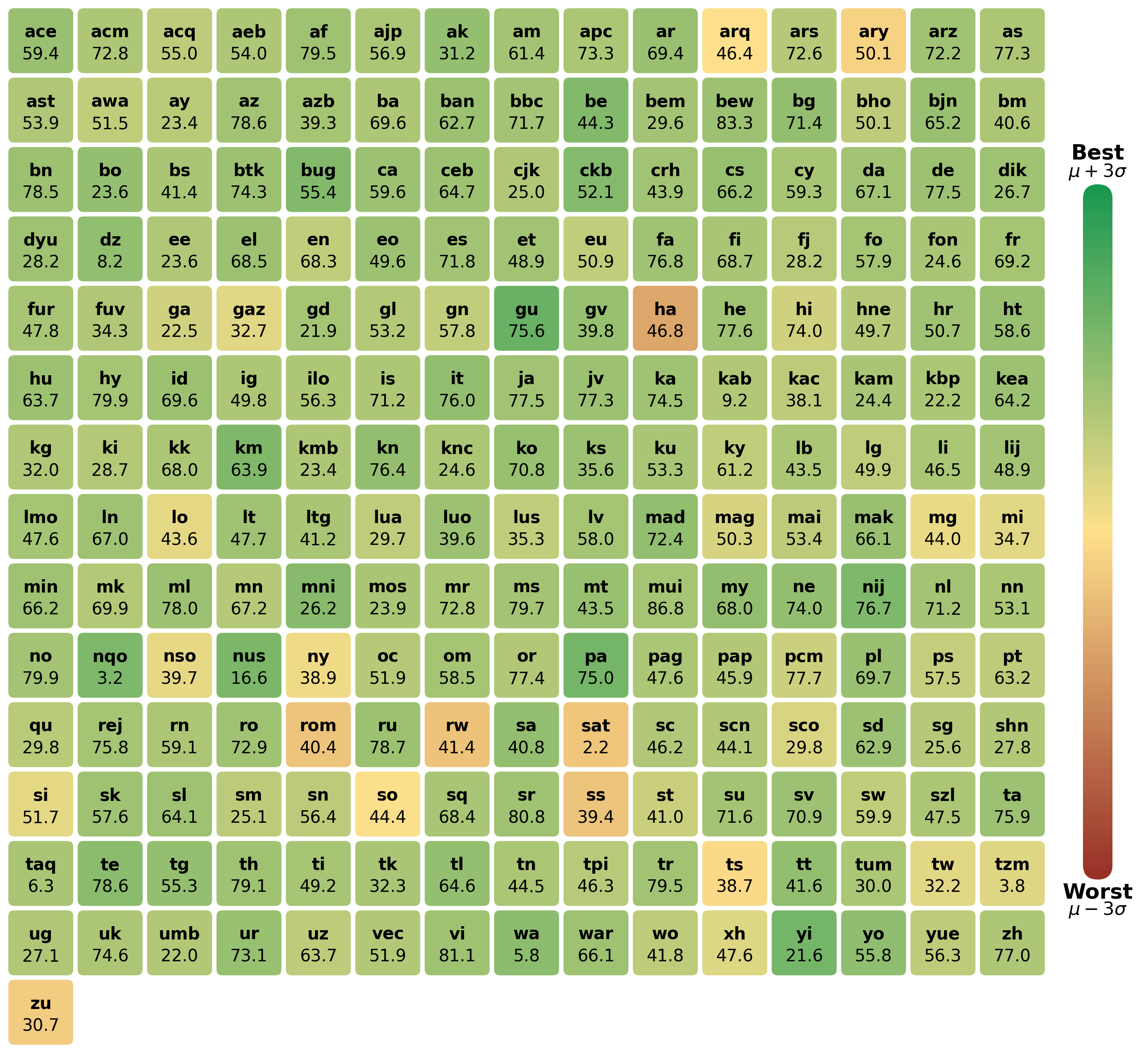</details> Figure 2: Performance of j-v5-text-small on different languages on MMTEB compared to other models Table 2 does not provide insight into language-specific differences in performance, so we conducted separate analyses, calculating average scores for individual languages, for five small multilingual models with published scores for all MMTEB tasks: - Gemma-300M - Qwen3-0.6B (instr.) - BGE-M3 Chen et al. (2024) - jina-embeddings-v5-text-small - jina-embeddings-v5-text-nano Figure 2 presents the average scores per language for jina-embeddings-v5-text-small as a heat map, with colors them based on its performance compared to the other four models. Specifically, the color space is mapped to the interval $\mu± 3\sigma$ for each individual language. Appendix A.6 contains heat maps for all five models. Table 3: MTEB(eng, v2) Evaluation Results | Model | Params | Dim | Avg Tasks | Avg Type | Cls | Clu | Pair | RR | Ret | STS | Sum | | --- | --- | --- | --- | --- | --- | --- | --- | --- | --- | --- | --- | | Qwen3-4B | 4B | 2560 | 74.6 | 68.1 | 89.8 | 57.5 | 87.0 | 50.8 | 68.5 | 88.7 | 34.4 | | jina-v4 | 3.8B | 2048 | 65.09 | 60.68 | 74.1 † | 45.5 † | 83.1 † | 48.04 † | 56.2 | 85.9 | 32.0 † | | Qwen3-0.6B (instr.) | 596M | 1024 | 70.5 | 64.7 | 84.6 | 54.1 | 84.4 | 48.2 | 61.8 | 86.6 | 33.4 | | Qwen3-0.6B (generic) | 596M | 1024 | 67.0 | 62.0 | 72.0 † | 51.8 † | 84.4 | 46.2 † | 59.8 † | 86.6 | 33.4 | | jina-v3 | 572M | 1024 | 65.7 | 62.6 | 85.8 | 47.4 | 84.0 | 47.9 | 54.3 | 85.8 | 32.9 | | snowflake-l-v2 | 568M | 1024 | 63.6 | 59.8 | 73.4 | 44.4 | 83.0 | 47.5 | 58.6 | 78.1 | 33.8 | | mult.-e5-l-instr. | 560M | 1024 | 65.5 | 61.2 | 75.5 | 49.9 | 86.2 | 48.7 | 53.5 | 84.7 | 29.9 | | j-v5-text-small | 677M | 1024 | 71.7 | 65.6 | 90.4 | 54.7 | 85.0 | 49.4 | 60.1 | 88.1 | 31.8 | | KaLM-mini-v2.5 | 494M | 896 | 71.3 | 65.3 | 90.5 | 58.1 | 86.6 | 47.4 | 58.5 | 84.8 | 31.2 | | voyage-4-nano | 480M | 2048 | 63.3 | 58.8 | 73.9 † | 46.9 † | 83.0 † | 47.7 † | 52.3 † | 81.6 † | 26.2 † | | Gemma-300M | 308M | 768 | 69.7 | 65.1 | 87.6 | 56.6 | 87.3 | 47.4 | 55.7 | 83.6 | 37.6 | | j-v5-text-nano | 239M | 768 | 71.0 | 65.2 | 89.7 | 53.5 | 84.7 | 49.2 | 58.8 | 88.3 | 31.9 | Task Abbreviations: Avg Tasks: Average (Task), Avg Type: Average (Task Type), Cls: Classification, Clu: Clustering, Pair: Pair Classification, RR: Reranking, Ret: Retrieval, STS: Semantic Textual Similarity, Sum: Summarization † (partially) self-evaluated Table 3 presents the English MTEB benchmark results for all included models. For results on individual tasks, see Appendix A.2. Here, jina-embeddings-v5-text-small achieves the highest average score among the small multilingual models, but a lower score than Qwen3-4B. When examining specific task categories, Qwen3-0.6B achieves slightly better retrieval performance when used with instructions, and multilingual-e5-large-instruct obtains the best results on pair classification tasks. Using Qwen3-0.6B without individual instructions for each task leads to a similar loss of performance for English benchmarks as was observed for MMTEB. Among models with fewer than 500M parameters, KaLM-mini-v2.5 achieves the highest average scores, only slightly better than jina-embeddings-v5-text-nano, despite having more than twice as many parameters. jina-embeddings-v5-text-nano achieves higher performance than all other models under 0.5B parameters in retrieval, reranking, and STS tasks. We note that Gemma-300M has the highest overall performance on summarization. 5.2 Performance on Various Retrieval Benchmarks Table 4: Retrieval Benchmark Results | Model | Params | Dim | Avg Tasks | MTEB-M | MTEB-E | RTEB | BEIR | Long | | --- | --- | --- | --- | --- | --- | --- | --- | --- | | Qwen3-4B | 4B | 2560 | 67.95 | 69.60 | 68.46 | 70.77 † | 61.58 | 78.82 † | | jina-v4 | 3.8B | 2048 | 63.62 | 66.43 | 56.15 | 66.52 | 53.97 † | 69.88 | | Qwen3-0.6B | 596M | 1024 | 61.87 | 64.65 | 61.83 | 64.21 † | 55.52 | 72.20 † | | jina-v3 | 572M | 1024 | 56.11 | 55.76 | 54.29 | 54.58 † | 53.17 | 55.67 | | snowflake-l-v2 | 568M | 1024 | 57.59 | 58.36 | 58.56 | 53.95 | 55.22 | 63.74 | | mult.-e5-l-instr. | 560M | 1024 | 54.22 | 57.12 | 53.47 | 54.78 | 52.74 | 41.76 | | j-v5-text-small | 677M | 1024 | 63.28 | 64.88 | 60.07 | 66.84 | 56.67 | 66.39 | | KaLM-mini-v2.5 | 494M | 896 | 56.58 | 57.90 | 58.45 | 56.51 † | 55.00 † | 43.35 † | | voyage-4-nano | 480M | 2048 | 61.48 | 63.58 † | 52.30 † | 70.36 † | 49.93 † | 74.93 † | | Gemma-300M | 308M | 768 | 59.66 | 62.49 | 55.69 | 63.75 † | 53.69 † | 55.29 † | | j-v5-text-nano | 239M | 768 | 61.43 | 63.26 | 58.80 | 64.08 | 56.06 | 63.65 | Task Abbreviations: Avg Tasks: Task-level mean across benchmarks, MTEB-M: MTEB Multilingual v2, MTEB-E: MTEB English v2, RTEB: RTEB (Multilingual, Public), BEIR: BEIR Retrieval, Long: LongEmbed † (partially) self-evaluated To provide a more global view of model performance, we used three additional benchmarks: RTEB (Multilingual) This benchmark contains a mixture of publicly-available tasks and additional private tasks. These scores here refer to only the public tasks because we do not have access to the private ones. Liu et al. (2025), BeIR Thakur et al. , and LongEmbed Zhu et al. (2024). We summarize the results together with the retrieval scores on the MTEB benchmarks from Section 5.1 in Table 4. Detailed results for individual datasets are presented in Appendix A.4 In contrast to the MTEB retrieval benchmarks, BeIR contains very large English datasets, demonstrating the models’ performance on million document-scale corpora. LongEmbed contains tests on relatively long documents when most benchmarks only contain passages. RTEB’s tests emphasize model performance on enterprise use cases. jina-embeddings-v5-text-small achieves the highest task-level average across all retrieval benchmarks among the models tested, outperforming comparably-sized Qwen3-0.6B on three out of five benchmarks. Qwen3-0.6B enjoys stronger scores on MTEB English and LongEmbed, suggesting that it has an advantage on English and long-document retrieval tasks. Both jina-embeddings-v5-text models substantially outperform jina-v3, snowflake-L-v2, and multilingual e5-large-instruct. Among models with under 500M parameters, jina-embeddings-v5-text-nano achieves the best BEIR and MTEB English scores while being the smallest model tested. Voyage-4-nano has a slightly higher task-level average than jina-embeddings-v5-text-nano and significantly higher scores on RTEB and LongEmbed. However, voyage-4-nano is roughly twice the size of j-v5-text-nano and has an embedding dimensionality of 2048 compared to jina-embeddings-v5-text-nano ’s 768. Gemma-300M and KaLM-mini-v2.5 also achieve competitive results on individual benchmarks but fall behind for the overall average across benchmarks. The Qwen3-4B teacher model unsurprisingly achieves the best results across all benchmarks by a considerable margin. 5.3 Ablation Studies We analyzed the effect of key design choices in our training setup through ablation testing. We focused on several factors that directly influence retrieval performance. Section 5.3.1 describes empirical studies on different distillation strategies and Section 5.3.2 studies the role of student and teacher projections for aligning embedding spaces during distillation. Furthermore, in Section 5.3.3, we investigate the influence of the three loss components used to train the retrieval adapter, and in Section 5.3.4 how GOR regularization makes the model more robust towards binary quantization. 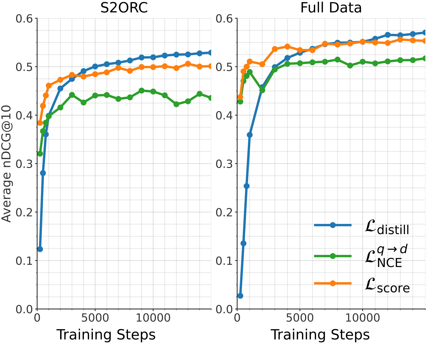5.3.1 Comparison of Training Objectives We studied the impact of different training objectives on retrieval performance by comparing three distinct loss functions: InfoNCE $\mathcal{L}_{\text{NCE}}^{q→ d}$ (see Equation (2)), embedding-based distillation $\mathcal{L}_{\mathrm{distill}}$ (see Equation (1)), and score-based distillation $\mathcal{L}_{\mathrm{score}}$ . All models are evaluated on the MTEB English v2 retrieval benchmark, with nDCG@10 reported across training steps. Score-based distillation loss: As an alternative to direct embedding alignment with $\mathcal{L}_{\mathrm{distill}}$ , we evaluated a score-based distillation loss that aims to match the distribution of pairwise similarities produced by the teacher and student models. Specifically, we compute the Mean Squared Error (MSE) between the softmax-normalized similarity matrices: $$ \mathcal{L}_{\mathrm{score}}=\sum_{\mathbf{z}\in\{\mathbf{x},\mathbf{y}\}}\frac{1}{B}\sum_{i=1}^{B}\sum_{j=1}^{B}\Bigl(p^{S}_{i,j}(\mathbf{z})-p^{T}_{i,j}(\mathbf{z})\Bigr)^{2} \tag{9} $$ where the probability distributions $p^{\alpha}_{i,j}$ for student model ( $S$ ) and teacher model ( $T$ ) are defined as: $$ p^{\alpha}_{i,j}(\mathbf{z})=\frac{\exp\!\bigl(\phi(\mathbf{z}^{\alpha}_{i},\,\mathbf{z}^{\alpha}_{j})/\tau\bigr)}{\sum_{k=1}^{B}\exp\!\bigl(\phi(\mathbf{z}^{\alpha}_{i},\,\mathbf{z}^{\alpha}_{k})/\tau\bigr)},\;\alpha\in\{S,T\}. \tag{10} $$ Here, $\phi$ denotes the cosine similarity and $\tau$ is a temperature hyperparameter. To emphasize the importance of higher similarity scores compared to lower similarity scores, we use temperature-scaled softmax values with $\tau=0.02$ . <details> <summary>x1.png Details</summary>  ### Visual Description ## Line Chart: Training Performance Comparison ### Overview The image presents two line charts comparing the training performance of different loss functions on two datasets: S2ORC and Full Data. The performance metric is Average nDCG@10, plotted against Training Steps. Each chart displays three loss functions: $\mathcal{L}_{distill}$, $\mathcal{L}^{q \rightarrow d}_{NCE}$, and $\mathcal{L}_{score}$. ### Components/Axes * **X-axis:** Training Steps (ranging from 0 to approximately 10,000) * **Y-axis:** Average nDCG@10 (ranging from 0.0 to 0.6) * **Left Chart Title:** S2ORC * **Right Chart Title:** Full Data * **Legend:** Located on the bottom-right of the image. * Blue Line: $\mathcal{L}_{distill}$ (Distillation Loss) * Green Line: $\mathcal{L}^{q \rightarrow d}_{NCE}$ (NCE Loss) * Orange Line: $\mathcal{L}_{score}$ (Score Loss) ### Detailed Analysis or Content Details **S2ORC Chart (Left):** * **$\mathcal{L}_{distill}$ (Blue Line):** Starts at approximately 0.42, increases rapidly to around 0.54 by 2000 training steps, then plateaus around 0.55-0.57 for the remainder of the training. * **$\mathcal{L}^{q \rightarrow d}_{NCE}$ (Green Line):** Begins at approximately 0.41, increases to around 0.48 by 2000 training steps, then fluctuates between 0.45 and 0.49, showing a slight downward trend after 8000 steps. * **$\mathcal{L}_{score}$ (Orange Line):** Starts at approximately 0.45, increases to around 0.52 by 2000 training steps, then plateaus around 0.52-0.54 for the remainder of the training. **Full Data Chart (Right):** * **$\mathcal{L}_{distill}$ (Blue Line):** Starts at approximately 0.38, increases rapidly to around 0.56 by 2000 training steps, then plateaus around 0.57-0.60 for the remainder of the training. * **$\mathcal{L}^{q \rightarrow d}_{NCE}$ (Green Line):** Begins at approximately 0.40, increases to around 0.50 by 2000 training steps, then fluctuates between 0.50 and 0.54, showing a slight upward trend after 8000 steps. * **$\mathcal{L}_{score}$ (Orange Line):** Starts at approximately 0.42, increases to around 0.53 by 2000 training steps, then plateaus around 0.53-0.56 for the remainder of the training. ### Key Observations * In both datasets, $\mathcal{L}_{distill}$ consistently achieves the highest Average nDCG@10, indicating superior performance compared to the other loss functions. * The performance gap between the loss functions appears to be more pronounced in the "Full Data" chart than in the "S2ORC" chart. * All loss functions exhibit diminishing returns after approximately 2000 training steps, suggesting that further training may not yield significant improvements. * $\mathcal{L}^{q \rightarrow d}_{NCE}$ shows more fluctuation in performance compared to the other two loss functions, particularly in the S2ORC dataset. ### Interpretation The charts demonstrate the effectiveness of the distillation loss ($\mathcal{L}_{distill}$) in improving the ranking performance of the model on both the S2ORC and Full Data datasets. The higher nDCG@10 values achieved by $\mathcal{L}_{distill}$ suggest that it is better at learning to rank relevant documents higher than irrelevant ones. The difference in performance between the two datasets could be attributed to the size and diversity of the data. The "Full Data" dataset likely contains more examples and a wider range of document types, which allows the model to learn more robust ranking functions. The plateauing of performance after 2000 training steps suggests that the model is approaching its capacity on these datasets. Further improvements may require more complex model architectures, larger datasets, or different training strategies. The fluctuations observed in $\mathcal{L}^{q \rightarrow d}_{NCE}$ could indicate instability during training, potentially due to the specific properties of the NCE loss function or the dataset. </details> Figure 3: Performance comparison of different training objectives. Average nDCG@10 on the MTEB (English, v2) benchmark for S2ORC (left) and the full training data mixture (right). We conducted these experiments under two data regimes: a filtered version of the S2ORC dataset https://huggingface.co/datasets/sentence-transformers/s2orc (Last Access: 02/09/2026) and the full data mixture used during the first stage of our training. Detailed hyperparameter configurations for each objective and extended results at different learning rates are provided in Appendix A.5. Figure 3 illustrates training progress for all three loss functions on the MTEB English v2 retrieval benchmark at nDCG@10. We observe clear differences in both convergence speed and final performance. While $\mathcal{L}_{\text{score}}$ and $\mathcal{L}_{\text{NCE}}$ provide a significantly faster initial increase in scores, they plateau relatively early, with score-based distillation showing very limited progress in later stages. In contrast, embedding-based distillation ( $\mathcal{L}_{\text{distill}}$ ) converges more slowly at the beginning, yet improves steadily and ultimately achieves the highest final retrieval performance in both data regimes. This suggests that while score-level matching is efficient for early alignment, directly aligning student and teacher embeddings provides a stronger and more sustained supervisory signal for long-term refinement. 5.3.2 Projection Layer <details> <summary>img/s2orc_projection1.png Details</summary>  ### Visual Description \n ## Line Chart: Average nDCG@10 vs. Training Steps ### Overview This image presents a line chart illustrating the performance of "Student" and "Teacher" models, both in "frozen" and "trainable" projection states, as measured by Average nDCG@10 over a range of Training Steps. The chart aims to compare the learning curves of these different configurations. ### Components/Axes * **X-axis:** Training Steps, ranging from 0 to approximately 6000, with tick marks at 0, 1000, 2000, 3000, 4000, 5000, and 6000. * **Y-axis:** Average nDCG@10, ranging from 0 to 0.6, with tick marks at 0, 0.1, 0.2, 0.3, 0.4, 0.5, and 0.6. * **Legend:** Located at the bottom-right of the chart. It contains the following labels and corresponding colors: * Student (proj. frozen) - Blue * Student (proj. trainable) - Green * Teacher (proj. frozen) - Orange * Teacher (proj. trainable) - Red * **Grid:** A light gray grid is present across the chart, aiding in value estimation. ### Detailed Analysis The chart displays four distinct lines, each representing a different model configuration. * **Student (proj. frozen) - Blue Line:** This line starts at approximately 0.18 at 0 Training Steps and rapidly increases to around 0.45 by 1000 Training Steps. It continues to rise, reaching approximately 0.53 by 4000 Training Steps, and plateaus around 0.54-0.55 for the remainder of the training period. * **Student (proj. trainable) - Green Line:** This line begins at approximately 0.12 at 0 Training Steps and exhibits a slower initial increase compared to the frozen student. It reaches around 0.40 by 1000 Training Steps, and continues to climb, eventually surpassing the frozen student, reaching approximately 0.55 by 4000 Training Steps. It plateaus around 0.56-0.57 for the remainder of the training period. * **Teacher (proj. frozen) - Orange Line:** This line starts at approximately 0.02 at 0 Training Steps and shows a very slow initial increase. It reaches around 0.45 by 4000 Training Steps and plateaus around 0.48-0.50 for the remainder of the training period. * **Teacher (proj. trainable) - Red Line:** This line begins at approximately 0.03 at 0 Training Steps and exhibits a slow initial increase. It reaches around 0.47 by 4000 Training Steps and plateaus around 0.50-0.52 for the remainder of the training period. ### Key Observations * The "trainable" projections consistently outperform the "frozen" projections for both Student and Teacher models. * The Student model, regardless of projection state, generally outperforms the Teacher model. * The Student (proj. trainable) line shows the highest overall performance, reaching the highest nDCG@10 value. * The Teacher (proj. frozen) line shows the lowest overall performance, reaching the lowest nDCG@10 value. * All lines exhibit diminishing returns in performance as training progresses beyond 4000 steps, indicating convergence. ### Interpretation The data suggests that allowing the projection layers to be trainable during training leads to improved performance (higher nDCG@10) for both Student and Teacher models. The Student model, in general, demonstrates a stronger learning capacity than the Teacher model, potentially due to differences in model architecture or initialization. The plateauing of the lines after 4000 training steps indicates that the models are converging and further training may not yield significant improvements. The initial low performance of the Teacher (proj. frozen) model suggests that the frozen projection layers are not effectively capturing the relevant information for the task. The difference in performance between the frozen and trainable models highlights the importance of adapting the projection layers to the specific training data. This could be due to the projection layers learning to better represent the data in a way that is more suitable for the downstream task. 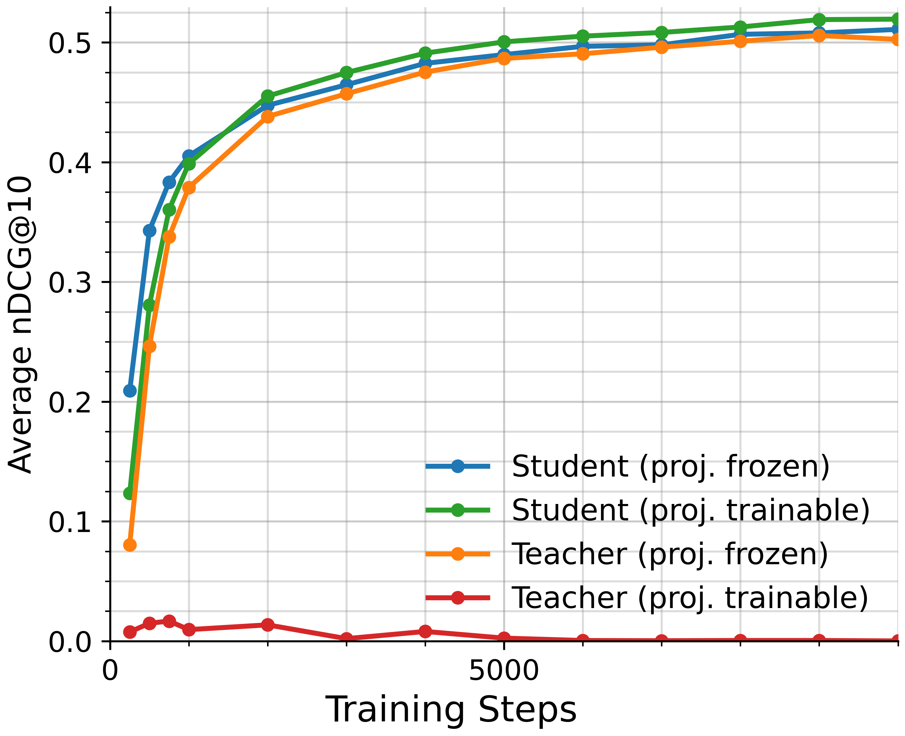</details> Figure 4: Comparison of projection configurations on S2ORC. Performance is measured by average nDCG@10 on MTEB (English, v2). We study the effect of projection head placement in embedding-based distillation when aligning models with mismatched embedding dimensions. All experiments use embedding-based distillation and the S2ORC dataset with the same hyperparameters used for the experiments in Section 5.3.1. We consider two projection strategies to align the embedding spaces: student projection, where the student’s embeddings are projected into the teacher’s embedding space before computing the distillation loss, and teacher projection, where the teacher’s embeddings are projected into the student’s embedding space. In both cases, we evaluated configurations with randomly initialized projections, and with the heads frozen and unfrozen, resulting in four experimental settings. As shown in Figure 4, we observe that while teacher projection without freezing simply does not work The training probably collapses into a trivial solution., all three other configurations perform comparably well. Freezing the student projection leads to faster convergence, and leaving it unfrozen yields the best final results. 5.3.3 Retrieval Loss Components Table 5: Evaluation of retrieval adapter training losses on MTEB v2 Retrieval subset and public RTEB tasks. | Loss Configuration | MTEB | RTEB | | --- | --- | --- | | $\mathcal{L}_{\text{NCE}}+\mathcal{L}_{\text{distill}}+\mathcal{L}_{\text{GOR}}$ | 64.50 | 66.45 | | $\mathcal{L}_{\text{NCE}}+\mathcal{L}_{\text{distill}}$ | 64.21 | 66.16 | | $\mathcal{L}_{\text{NCE}}+\mathcal{L}_{\text{GOR}}$ | 64.11 | 66.11 | | $\mathcal{L}_{\text{distill}}+\mathcal{L}_{\text{GOR}}$ | 63.49 | 65.05 | | $\mathcal{L}_{\text{NCE}}$ | 63.38 | 65.14 | | $\mathcal{L}_{\text{distill}}$ | 63.16 | 64.37 | Table 6: Impact of GOR loss on quantization robustness, evaluated on MTEB v2 Retrieval subset and public RTEB tasks. | | MTEB | RTEB | | | | --- | --- | --- | --- | --- | | Configuration | BF16 | Binary | BF16 | Binary | | Full (w/ GOR) | 64.50 | 62.60 (-1.90) | 66.45 | 63.94 (-2.51) | | w/o GOR | 64.21 | 61.13 (-3.08) | 66.16 | 62.24 (-3.92) | Table 5 presents an ablation study on the components of our retrieval adapter training loss. We systematically remove individual losses from the full combination (Equation 4) to assess their individual contributions. The results show that combining all three losses yields the best performance across both benchmarks. Notably, we show that relying solely on embedding distillation is insufficient, as $\mathcal{L}_{\text{distill}}$ alone has the lowest scores (63.16 on MTEB, 64.37 on RTEB) of our tested combinations. This validates our two-stage training approach. While $\mathcal{L}_{\text{distill}}$ distillation provides strong initialization in stage 1 training, the addition of task-specific losses ( $\mathcal{L}_{\text{NCE}}$ and $\mathcal{L}_{\text{GOR}}$ ) in stage 2 is critical for maximizing retrieval performance. 5.3.4 GOR Loss and Quantization Robustness In Table 6, we present the results of training the model with and without the GOR loss component of Equation 4, both at full-precision (BF16) and binary quantization. At full precision, $\mathcal{L}_{\text{GOR}}$ contributes only modestly to performance, improving MTEB scores from 64.21 to 64.50 and RTEB from 66.16 to 66.45. However, its benefit becomes evident under quantization. Without $\mathcal{L}_{\text{GOR}}$ , performance degrades over 50% more on both MTEB and RTEB benchmarks, from -1.90 to -3.08 on MTEB and from -2.51 to -3.92 on RTEB. This robustness was the goal of GOR regularization: Ensuring fuller use of the available dimensions in embedding space, making the resulting representations less sensitive to information loss. 5.4 Truncation Robustness of Embeddings We evaluated the performance of truncated embeddings, the result of using Matryoshka Representation Learning Kusupati et al. (2022). We progressively reduced to smaller dimensions, in order to assess the efficiency and adaptability of the model’s latent space. Figure 5 shows scores on MMTEB’s retrieval benchmarks for embeddings of varying sizes, providing us with a systematic and quantitative analysis of the trade-off between retrieval accuracy and computational efficiency. <details> <summary>x2.png Details</summary>  ### Visual Description \n ## Line Chart: MMTEB Score vs. Truncate Dimension ### Overview This line chart depicts the relationship between the "Truncate Dimension" and the "MMTEB Score" for two different models: "j-v5-text-small" and "j-v5-text-nano". The chart shows how the MMTEB score changes as the truncate dimension is reduced. ### Components/Axes * **X-axis:** "Truncate Dimension" with markers at 1024, 768, 512, 256, and 32. * **Y-axis:** "MMTEB Score" with a scale ranging from approximately 0.4 to 0.65. * **Legend:** Located in the bottom-left corner, identifying two data series: * "j-v5-text-small" (represented by a magenta/purple line with diamond markers) * "j-v5-text-nano" (represented by a blue line with circular markers) * **Gridlines:** A light gray grid is present to aid in reading values. ### Detailed Analysis **j-v5-text-small (Magenta Line with Diamond Markers):** The line starts at approximately 0.65 at a truncate dimension of 1024. It remains relatively stable, fluctuating around 0.63-0.64 until a truncate dimension of 256. At 256, the line begins to decline, reaching approximately 0.58. At a truncate dimension of 32, the score drops to approximately 0.60. * 1024: 0.65 * 768: 0.64 * 512: 0.63 * 256: 0.62 * 32: 0.60 **j-v5-text-nano (Blue Line with Circular Markers):** The line begins at approximately 0.64 at a truncate dimension of 1024. It remains relatively stable, fluctuating around 0.63-0.64 until a truncate dimension of 256. At 256, the line begins to decline, reaching approximately 0.59. At a truncate dimension of 32, the score drops sharply to approximately 0.44. * 1024: 0.64 * 768: 0.64 * 512: 0.63 * 256: 0.60 * 32: 0.44 ### Key Observations * Both models exhibit a general trend of decreasing MMTEB score as the truncate dimension decreases. * The "j-v5-text-nano" model experiences a much more significant drop in MMTEB score at a truncate dimension of 32 compared to the "j-v5-text-small" model. * For truncate dimensions of 1024, 768, 512, and 256, the MMTEB scores for both models are relatively close. ### Interpretation The data suggests that reducing the truncate dimension impacts the performance of both models, as measured by the MMTEB score. However, the "j-v5-text-nano" model is more sensitive to this reduction, experiencing a substantial performance loss at lower dimensions. This could indicate that the "j-v5-text-nano" model relies more heavily on the higher dimensions for its performance, or that it has a lower capacity to retain information when dimensionality is reduced. The relatively stable performance of both models at higher truncate dimensions (1024, 768, 512, 256) suggests that these dimensions contribute to a baseline level of performance, but that further dimensionality reduction leads to diminishing returns and, eventually, significant performance degradation, particularly for the "j-v5-text-nano" model. The sharp decline of the blue line at 32 is a notable outlier, indicating a critical threshold for this model. </details> Figure 5: Average MMTEB score across reduced embedding dimensions. Our results show a sizable decline in retrieval performance when the embedding dimensions fall below 256. This aligns with expectations from the Johnson-Lindenstrauss Lemma (Johnson and Lindenstrauss, 1984), which establishes theoretical limits on dimensionality reduction while maintaining pairwise distances between data points. 6 Conclusion We have introduced two compact multilingual embedding models jina-embeddings-v5-text-small and jina-embeddings-v5-text-nano, and a novel training method for them that combines distillation-based and task-specific training. We demonstrate through extensive ablation studies that this approach outperforms existing alternatives. Our models achieve state-of-the-art performance among comparable multilingual embedding models and remain robust under truncation and binary quantization, with only minimal performance degradation in response to large increases in storage and computational efficiency. To support reproducibility and accelerate future research, we have released the models publicly along with out-of-the-box integration with Sentence Transformers (Reimers and Gurevych, 2019) and vLLM (Kwon et al., 2023), in addition to multiple quantized variants for llama.cpp ggml-org and contributors (2026). References - E. Agirre, D. Cer, M. Diab, and A. Gonzalez-Agirre (2012) SemEval-2012 Task 6: A Pilot on Semantic Textual Similarity. In SEM 2012: 1st Joint Conference on Lexical and Computational Semantics (SemEval), Cited by: §4.2.2. - N. Boizard, H. Gisserot-Boukhlef, D. M. Alves, A. Martins, A. Hammal, C. Corro, C. Hudelot, E. Malherbe, E. Malaboeuf, F. Jourdan, et al. (2025) EuroBERT: scaling multilingual encoders for european languages. arXiv preprint arXiv:2503.05500. Cited by: §3, §4. - J. Chen, S. Xiao, P. Zhang, K. Luo, D. Lian, and Z. Liu (2024) M3-embedding: multi-linguality, multi-functionality, multi-granularity text embeddings through self-knowledge distillation. In Findings of the Association for Computational Linguistics: ACL 2024, L. Ku, A. Martins, and V. Srikumar (Eds.), Bangkok, Thailand, pp. 2318–2335. Cited by: §2.3, 3rd item. - X. Chen, B. He, K. Hui, L. Sun, and Y. Sun (2021) Simplified tinybert: knowledge distillation for document retrieval. In European Conference on Information Retrieval, pp. 241–248. Cited by: §2.1. - [5] K. Enevoldsen, I. Chung, I. Kerboua, M. Kardos, A. Mathur, D. Stap, J. Gala, W. Siblini, D. Krzemiński, G. I. Winata, et al. MMTEB: massive multilingual text embedding benchmark. In The Thirteenth International Conference on Learning Representations, Cited by: §1, §5. - [6] P. Formont, M. DARRIN, B. Karimian, E. Granger, J. C. Cheung, I. B. Ayed, M. Shateri, and P. Piantanida Learning task-agnostic representations through multi-teacher distillation. In The Thirty-ninth Annual Conference on Neural Information Processing Systems, Cited by: §2.2. - ggml-org and contributors (2026) Llama.cpp: llm inference in c/c++. Note: https://github.com/ggml-org/llama.cpp GitHub repository, Accessed: 2026-02-16 Cited by: §6. - M. Günther, S. Sturua, M. K. Akram, I. Mohr, A. Ungureanu, B. Wang, S. Eslami, S. Martens, M. Werk, N. Wang, et al. (2025) Jina-embeddings-v4: universal embeddings for multimodal multilingual retrieval. In Proceedings of the 5th Workshop on Multilingual Representation Learning (MRL 2025), pp. 531–550. Cited by: §5. - S. Hofstätter, S. Althammer, M. Schröder, M. Sertkan, and A. Hanbury (2020) Improving efficient neural ranking models with cross-architecture knowledge distillation. arXiv preprint arXiv:2010.02666. Cited by: §2.2. - X. Jiao, Y. Yin, L. Shang, X. Jiang, X. Chen, L. Li, F. Wang, and Q. Liu (2020) Tinybert: distilling bert for natural language understanding. In Findings of the association for computational linguistics: EMNLP 2020, pp. 4163–4174. Cited by: §2.1. - W. Johnson and J. Lindenstrauss (1984) Extensions of lipschitz maps into a hilbert space. Contemporary Mathematics 26, pp. 189–206. Cited by: §5.4. - V. Karpukhin, B. Oguz, S. Min, P. S. Lewis, L. Wu, S. Edunov, D. Chen, and W. Yih (2020) Dense passage retrieval for open-domain question answering.. In EMNLP (1), pp. 6769–6781. Cited by: §4.2.1. - S. Kim, A. S. Rawat, M. Zaheer, S. Jayasumana, V. Sadhanala, W. Jitkrittum, A. K. Menon, R. Fergus, and S. Kumar (2023) EmbedDistill: a geometric knowledge distillation for information retrieval. arXiv preprint arXiv:2301.12005. Cited by: §2.2. - A. Kusupati, G. Bhatt, et al. (2022) Matryoshka Representation Learning. In Advances in Neural Information Processing Systems (NeurIPS 2022), Cited by: §3, §5.4. - W. Kwon, Z. Li, S. Zhuang, Y. Sheng, L. Zheng, C. H. Yu, J. E. Gonzalez, H. Zhang, and I. Stoica (2023) Efficient memory management for large language model serving with pagedattention. In Proceedings of the ACM SIGOPS 29th Symposium on Operating Systems Principles, Cited by: §6. - F. Liu, K. C. Enevoldsen, S. R. Samoed, I. Chung, T. Aarsen, and Z. Fődi (2025) Hugging Face. Note: Accessed: 2026-02-11 Cited by: §5.2. - X. Liu, H. Yan, C. An, X. Qiu, and D. Lin (2024) Scaling laws of roPE-based extrapolation. In The Twelfth International Conference on Learning Representations, Cited by: §4.1.1. - M. Marelli, S. Menini, et al. (2014) A SICK cure for the evaluation of compositional distributional semantic models. In Ninth International Conference on Language Resources and Evaluation (LREC), Cited by: §4.2.2. - A. Menon, S. Jayasumana, A. S. Rawat, S. Kim, S. Reddi, and S. Kumar (2022) In defense of dual-encoders for neural ranking. In International Conference on Machine Learning, pp. 15376–15400. Cited by: §2.2. - I. Mohr, M. Krimmel, S. Sturua, M. K. Akram, A. Koukounas, M. Günther, G. Mastrapas, V. Ravishankar, J. F. Martínez, F. Wang, et al. (2024) Multi-task contrastive learning for 8192-token bilingual text embeddings. arXiv preprint arXiv:2402.17016. Cited by: §2.3. - N. Muennighoff, N. Tazi, L. Magne, and N. Reimers (2023) Mteb: massive text embedding benchmark. In Proceedings of the 17th Conference of the European Chapter of the Association for Computational Linguistics, pp. 2014–2037. Cited by: §5. - E. Musacchio, L. Siciliani, P. Basile, and G. Semeraro (2025) XVLM2Vec: adapting lvlm-based embedding models to multilinguality using self-knowledge distillation. arXiv preprint arXiv:2503.09313. Cited by: §2.2. - A. v. d. Oord, Y. Li, and O. Vinyals (2018) Representation learning with contrastive predictive coding. arXiv preprint arXiv:1807.03748. Cited by: §4.2.1. - W. Park, D. Kim, Y. Lu, and M. Cho (2019) Relational knowledge distillation. arXiv preprint arXiv:1904.05068. Cited by: §4.2.4. - F. Pedregosa, G. Varoquaux, A. Gramfort, V. Michel, B. Thirion, O. Grisel, M. Blondel, P. Prettenhofer, R. Weiss, V. Dubourg, et al. (2011) Scikit-learn: machine learning in python. the Journal of machine Learning research 12, pp. 2825–2830. Cited by: footnote 6. - N. Reimers and I. Gurevych (2019) Sentence-bert: sentence embeddings using siamese bert-networks. In Proceedings of the 2019 Conference on Empirical Methods in Natural Language Processing and the 9th International Joint Conference on Natural Language Processing (EMNLP-IJCNLP), pp. 3982–3992. Cited by: §1, §6. - V. Sanh, L. Debut, J. Chaumond, and T. Wolf (2019) DistilBERT, a distilled version of bert: smaller, faster, cheaper and lighter. arXiv preprint arXiv:1910.01108. Cited by: §2.1. - S. Sturua, I. Mohr, M. Kalim Akram, M. Günther, B. Wang, M. Krimmel, F. Wang, G. Mastrapas, A. Koukounas, N. Wang, et al. (2025) Jina embeddings v3: multilingual text encoder with low-rank adaptations. In European Conference on Information Retrieval, pp. 123–129. Cited by: §2.3, §3, 1st item. - H. Su, W. Shi, J. Kasai, Y. Wang, Y. Hu, M. Ostendorf, W. Yih, N. A. Smith, L. Zettlemoyer, and T. Yu (2023) One embedder, any task: instruction-finetuned text embeddings. In Findings of the Association for Computational Linguistics: ACL 2023, pp. 1102–1121. Cited by: §2.3. - J. Su, M. Ahmed, Y. Lu, S. Pan, W. Bo, and Y. Liu (2024) Roformer: enhanced transformer with rotary position embedding. Neurocomputing 568, pp. 127063. Cited by: §4.1.1. - [31] N. Thakur, N. Reimers, A. Rücklé, A. Srivastava, and I. Gurevych BEIR: a heterogeneous benchmark for zero-shot evaluation of information retrieval models. In Thirty-fifth Conference on Neural Information Processing Systems Datasets and Benchmarks Track (Round 2), Cited by: §5.2. - H. S. Vera, S. Dua, B. Zhang, D. Salz, R. Mullins, S. R. Panyam, S. Smoot, I. Naim, J. Zou, F. Chen, et al. (2025) Embeddinggemma: powerful and lightweight text representations. arXiv preprint arXiv:2509.20354. Cited by: §1, §2.3, §4.2.1, 6th item. - Voyage AI (2026) Voyage-4-nano. Note: https://huggingface.co/voyageai/voyage-4-nano State-of-the-art text embedding model with 32,000 token context length Cited by: 5th item. - L. Wang, N. Yang, X. Huang, L. Yang, R. Majumder, and F. Wei (2024) Multilingual e5 text embeddings: a technical report. arXiv preprint arXiv:2402.05672. Cited by: 3rd item. - W. Wang, F. Wei, L. Dong, H. Bao, N. Yang, and M. Zhou (2020) MINILM: deep self-attention distillation for task-agnostic compression of pre-trained transformers. In Proceedings of the 34th International Conference on Neural Information Processing Systems, pp. 5776–5788. Cited by: §2.1. - Z. Wang, J. Zhang, J. Feng, and Z. Chen (2014) Knowledge graph and text jointly embedding. In Proceedings of the 2014 conference on empirical methods in natural language processing (EMNLP), pp. 1591–1601. Cited by: §2.3. - A. Yang, A. Li, B. Yang, B. Zhang, B. Hui, B. Zheng, B. Yu, C. Gao, C. Huang, C. Lv, et al. (2025) Qwen3 technical report. arXiv preprint arXiv:2505.09388. Cited by: §3, §4. - E. Yang, D. Lawrie, J. Mayfield, D. W. Oard, and S. Miller (2024) Translate-distill: learning cross-language dense retrieval by translation and distillation. In European Conference on Information Retrieval, pp. 50–65. Cited by: §2.2. - P. Yu, L. Merrick, G. Nuti, and D. Campos (2024) Arctic-embed 2.0: multilingual retrieval without compromise. arXiv preprint arXiv:2412.04506. Cited by: 2nd item. - D. Zhang, J. Li, Z. Zeng, and F. Wang (2024a) Jasper and stella: distillation of sota embedding models. arXiv preprint arXiv:2412.19048. Cited by: §1, §2.2. - D. Zhang, Z. Zeng, Y. Zhou, and S. Lu (2025a) Jasper-token-compression-600m technical report. arXiv preprint arXiv:2511.14405. Cited by: §2.2. - K. Zhang, Y. Luan, H. Hu, K. Lee, S. Qiao, W. Chen, Y. Su, and M. Chang (2024b) MagicLens: self-supervised image retrieval with open-ended instructions. In Proceedings of the 41st International Conference on Machine Learning, pp. 59403–59420. Cited by: §2.3. - X. Zhang, Y. Zhang, D. Long, W. Xie, Z. Dai, J. Tang, H. Lin, B. Yang, P. Xie, F. Huang, et al. (2024c) MGTE: generalized long-context text representation and reranking models for multilingual text retrieval. In Proceedings of the 2024 Conference on Empirical Methods in Natural Language Processing: Industry Track, pp. 1393–1412. Cited by: §4.1.1. - X. Zhang, F. X. Yu, S. Kumar, and S. Chang (2017) Learning spread-out local feature descriptors. In Proceedings of the IEEE international conference on computer vision, pp. 4595–4603. Cited by: §4.2.1. - Y. Zhang, M. Li, D. Long, X. Zhang, H. Lin, B. Yang, P. Xie, A. Yang, D. Liu, J. Lin, et al. (2025b) Qwen3 embedding: advancing text embedding and reranking through foundation models. arXiv preprint arXiv:2506.05176. Cited by: §1, §4, 7th item, §5. - X. Zhao, X. Hu, Z. Shan, S. Huang, Y. Zhou, X. Zhang, Z. Sun, Z. Liu, D. Li, X. Wei, et al. (2025) Kalm-embedding-v2: superior training techniques and data inspire a versatile embedding model. arXiv preprint arXiv:2506.20923. Cited by: 4th item. - D. Zhu, L. Wang, N. Yang, Y. Song, W. Wu, F. Wei, and S. Li (2024) LongEmbed: extending embedding models for long context retrieval. In Proceedings of the 2024 Conference on Empirical Methods in Natural Language Processing, pp. 802–816. Cited by: §5.2. Appendix A Appendix A.1 Hyperparameters The following table outlines all hyperparameters used during the various training phases. For all the LoRA adapters we use a rank of 32 and an alpha value of 32. Table A1: Hyperparameters for the different models and training stages. | Stage | Model | Steps | Devices & Batch size | Max. Tokens (Seq. Length) | LR | $\theta$ | Others | | --- | --- | --- | --- | --- | --- | --- | --- | | First Stage | j-v5-text-small | 50,000 | 8 $×{}$ 512 | 512 | $1·{}10^{-4}$ | 1M | | | j-v5-text-nano | 50,000 | 8 $×{}$ 1024 | 512 | $1·{}10^{-4}$ | 250K | | | | Long Context | j-v5-text-small | 6,500 | 2 $×{}$ 64 | 4096 | $1·{}10^{-4}$ | 500K | | | Training | | | | | | | | | Asym. Retrieval | j-v5-text-small | 8,000 | 2 $×{}$ (256 / 64) | 384 / 4096 | $2·{}10^{-5}$ | 1M | $\tau=0.02,\lambda_{D}=2,$ | | j-v5-text-nano | 8,000 | 2 $×{}$ (384 / 96) | 384 / 4096 | $2·{}10^{-5}$ | 250K | $\lambda_{\text{NCE}}=\lambda_{S}=1$ | | | Text-Matching | j-v5-text-small | 20000 | 1 $×{}$ 256 | 384 | $5·{}10^{-5}$ | 1M | $\tau=0.02,\tau^{\prime}=0.05$ , | | j-v5-text-nano | 20000 | 1 $×{}$ 256 | 384 | $5·{}10^{-5}$ | 250K | $\lambda_{\text{NCE}}=1,\lambda_{D}=2$ | | | Clustering | j-v5-text-small | 20,000 | 1 $×{}$ 512 | 512 | $1·{}10^{-5}$ | 100K | | | j-v5-text-nano | 20,000 | 1 $×{}$ 1024 | 512 | $1·{}10^{-5}$ | 25K | | | | Classification | j-v5-text-small | 30,000 | 4 $×{}$ 64 | 512 | $4·{}10^{-4}$ | 3.5M | $\tau=0.02,$ | | j-v5-text-nano | 30,000 | 4 $×{}$ 128 | 512 | $4·{}10^{-4}$ | 1M | $\lambda_{\text{NCE}}=1,\lambda_{R}=20$ | | A.2 English MTEB Benchmarks The following evaluations are computed using the default metrics on the MTEB(eng, v2) benchmark. We either report results that are stated on the MTEB leaderboard https://huggingface.co/spaces/mteb/leaderboard (Last Access: 02/02/2026) or self-evaluate them using the mteb package https://github.com/embeddings-benchmark/mteb (Last Access: 02/02/2026). Table A2: Evaluation Results on MTEB Retrieval Tasks (nDCG@10 [%]) | Model | AVG | Arg | CQG | CQU | CFHN | FEV | FiQA | HPQA | SCI | TREC | TOU | | --- | --- | --- | --- | --- | --- | --- | --- | --- | --- | --- | --- | | Qwen3-4B | 68.46 | 75.64 | 71.51 | 59.60 | 48.48 | 92.47 | 62.65 | 75.22 | 31.44 | 92.92 | 74.65 | | jina-v4 | 56.15 | 66.96 | 57.59 | 42.95 | 34.57 | 87.69 | 48.49 | 69.01 | 21.48 | 80.36 | 52.41 | | Qwen3-0.6B (instr.) | 61.83 | 70.97 | 64.14 | 51.49 | 43.62 | 88.94 | 46.61 | 67.69 | 24.41 | 90.52 | 69.90 | | Qwen3-0.6B (generic) | 59.77 | 67.48 | 63.83 | 49.80 | 37.61 | 86.66 | 46.83 | 66.90 | 22.77 | 88.80 | 67.01 | | jina-v3 | 54.29 | 43.29 | 58.02 | 43.52 | 43.14 | 89.90 | 47.35 | 64.70 | 19.92 | 77.74 | 55.28 | | snowflake-l-v2 | 58.56 | 59.11 | 63.18 | 46.57 | 42.83 | 92.21 | 45.35 | 68.40 | 20.28 | 83.63 | 64.05 | | mult.-e5-l-instr. | 53.47 | 58.48 | 63.96 | 44.73 | 23.83 | 75.76 | 48.43 | 64.53 | 19.24 | 82.51 | 53.26 | | j-v5-text-small | 60.07 | 65.07 | 62.16 | 49.61 | 41.75 | 90.46 | 49.63 | 69.94 | 23.04 | 78.49 | 70.59 | | KaLM-mini-v2.5 | 58.45 | 60.15 | 65.52 | 48.87 | 35.06 | 88.23 | 47.10 | 71.79 | 21.62 | 82.98 | 63.23 | | voyage-4-nano | 52.30 | 58.63 | 60.96 | 46.15 | 22.41 | 68.14 | 50.99 | 63.25 | 21.28 | 77.89 | 53.83 | | Gemma-300M | 55.69 | 71.54 | 59.53 | 41.52 | 26.71 | 80.75 | 47.74 | 71.48 | 18.43 | 80.35 | 58.90 | | j-v5-text-nano | 58.80 | 65.70 | 61.60 | 47.40 | 40.03 | 89.82 | 47.85 | 69.28 | 22.60 | 77.60 | 66.12 | | v5-small stage 1 | 58.52 | 64.05 | 62.00 | 48.42 | 38.19 | 86.46 | 47.53 | 68.45 | 22.28 | 79.48 | 68.36 | | v5-nano stage 1 | 58.29 | 65.60 | 60.86 | 46.79 | 36.68 | 87.58 | 46.20 | 68.70 | 22.23 | 79.39 | 68.88 | Tasks: Avg: Average over all tasks, Arg: ArguAna, CQG: CQADupstackGamingRetrieval, CQU: CQADupstackUnixRetrieval, CFHN: ClimateFEVERHardNegatives, FEV: FEVERHardNegatives, FiQA: FiQA2018, HPQA: HotpotQAHardNegatives, SCI: SCIDOCS, TREC: TRECCOVID, TOU: Touche2020Retrieval.v3 Table A3: Evaluation Results on MTEB Reranking Tasks (MAP@1000 [%]). | Model | Avg | MindSmallReranking | AskUbuntuDupQuestions | | --- | --- | --- | --- | | Qwen3-4B | 50.76 | 32.71 | 68.81 | | jina-v4 | 48.04 | 32.51 | 63.56 | | Qwen3-0.6B (instr.) | 48.18 | 31.23 | 65.13 | | Qwen3-0.6B (generic) | 46.17 | 31.40 | 60.94 | | jina-v3 | 47.94 | 30.83 | 65.04 | | snowflake-l-v2 | 47.47 | 31.59 | 63.35 | | mult.-e5-l-instr. | 48.74 | 33.07 | 64.41 | | j-v5-text-small | 49.39 | 32.69 | 66.08 | | KaLM-mini-v2.5 | 47.42 | 32.45 | 62.39 | | voyage-4-nano | 47.68 | 32.19 | 63.18 | | Gemma-300M | 47.43 | 31.90 | 62.96 | | j-v5-text-nano | 49.23 | 32.72 | 65.73 | | v5-small stage 1 | 47.07 | 32.24 | 61.91 | | v5-nano stage 1 | 47.64 | 32.43 | 62.85 | Table A4: Evaluation Results on MTEB Semantic Textual Similarity Tasks (Spearman correlation [%]). | Model | Avg | BIO | SICK-R | STS12 | STS13 | STS14 | STS15 | STS17 | STS22 | STSB | | --- | --- | --- | --- | --- | --- | --- | --- | --- | --- | --- | | Qwen3-4B | 88.7 | 82.9 | 88.1 | 86.6 | 94.4 | 90.9 | 93.8 | 95.1 | 73.1 | 93.7 | | jina-v4 | 85.9 | 89.2 | 89.2 | 83.5 | 88.6 | 84.8 | 89.7 | 88.7 | 70.7 | 88.6 | | Qwen3-0.6B (instr.) | 86.6 | 85.5 | 84.8 | 83.0 | 91.8 | 87.1 | 91.4 | 93.3 | 71.1 | 91.1 | | Qwen3-0.6B (generic) | 86.6 | 85.5 | 84.8 | 83.0 | 91.8 | 87.1 | 91.5 | 93.2 | 71.1 | 91.1 | | jina-v3 | 85.8 | 88.7 | 89.6 | 82.4 | 89.5 | 85.0 | 89.3 | 90.0 | 68.4 | 89.4 | | snowflake-l-v2 | 78.0 | 87.2 | 74.0 | 71.2 | 80.4 | 75.1 | 82.9 | 84.5 | 67.9 | 79.2 | | mult.-e5-l-instr. | 84.7 | 87.5 | 81.7 | 82.5 | 88.1 | 84.8 | 91.0 | 90.3 | 68.2 | 88.4 | | j-v5-text-small | 88.1 | 85.2 | 91.6 | 85.1 | 88.7 | 88.5 | 92.6 | 94.9 | 71.8 | 94.8 | | KaLM-mini-v2.5 | 84.8 | 84.0 | 83.2 | 81.9 | 89.5 | 86.0 | 90.3 | 92.3 | 67.2 | 88.9 | | voyage-nano | 81.6 | 86.6 | 77.9 | 76.0 | 87.4 | 80.2 | 86.2 | 88.9 | 67.0 | 84.5 | | Gemma-300m | 83.6 | 86.4 | 81.4 | 79.3 | 86.4 | 83.7 | 89.3 | 90.3 | 67.5 | 88.2 | | j-v5-text-nano | 88.3 | 87.5 | 92.0 | 85.3 | 89.5 | 88.9 | 92.8 | 93.7 | 70.4 | 94.5 | | v5-small stage 1 | 82.3 | 87.3 | 78.2 | 77.3 | 84.3 | 80.1 | 88.2 | 84.9 | 72.1 | 88.0 | | v5-nano stage 1 | 83.6 | 87.5 | 81.0 | 80.3 | 86.7 | 81.6 | 88.9 | 90.1 | 68.6 | 87.8 | Tasks: Avg: Average over all tasks, BIO: BIOSSES, STS22: STS22v2, STSB: STSBenchmark Table A5: Evaluation Results on MTEB Pair Classification Tasks (Max Average Precision [%]). | Model | Avg | SprintDuplicateQuestions | TwitterSemEval2015 | TwitterURLCorpus | | --- | --- | --- | --- | --- | | Qwen3-4B | 87.0 | 96.1 | 77.8 | 87.2 | | jina-v4 | 83.1 | 91.4 | 71.5 | 86.4 | | Qwen3-0.6B (instr.) | 84.4 | 94.1 | 72.3 | 86.8 | | Qwen3-0.6B (generic) | 84.4 | 94.1 | 72.3 | 86.8 | | jina-v3 | 84.0 | 97.0 | 70.9 | 84.1 | | snowflake-l-v2 | 83.0 | 96.5 | 67.0 | 85.4 | | mult.-e5-l-instr. | 86.2 | 92.2 | 79.8 | 86.7 | | j-v5-text-small | 85.0 | 96.6 | 72.3 | 86.0 | | KaLM-mini-v2.5 | 86.6 | 96.1 | 77.2 | 86.7 | | voyage-nano | 83.0 | 93.2 | 70.5 | 86.7 | | Gemma-300m | 87.3 | 97.0 | 77.9 | 86.9 | | j-v5-text-nano | 84.7 | 95.5 | 73.1 | 85.6 | | v5-small stage 1 | 83.4 | 96.4 | 68.4 | 85.5 | | v5-nano stage 1 | 83.4 | 96.9 | 67.6 | 85.6 | Avg: Average over all tasks Table A6: Evaluation Results on MTEB Classification Tasks (Accuracy [%]). | Model | Avg | AmzCF | Bnk77 | IMDB | MTOP | M-Int | M-Scn | Tox | TwSent | | --- | --- | --- | --- | --- | --- | --- | --- | --- | --- | | Qwen3-4B | 89.8 | 93.7 | 86.3 | 97.2 | 97.8 | 85.0 | 88.8 | 91.4 | 78.4 | | jina-v4 | 74.1 | 72 | 78.6 | 81.0 | 93.2 | 70.5 | 72.6 | 64.5 | 60.3 | | Qwen3-0.6B (instr.) | 84.6 | 91.5 | 81.0 | 95.4 | 96.0 | 80.4 | 74.1 | 82.1 | 76.0 | | Qwen3-0.6B (generic) | 72.0 | 70.1 | 71.6 | 89.6 | 91.0 | 50.0 | 74.4 | 68.0 | 61.5 | | jina-v3 | 85.8 | 90.9 | 84.1 | 91.9 | 97.5 | 75.2 | 84.1 | 91.3 | 71.4 | | snowflake-l-v2 | 73.4 | 65.6 | 81.8 | 72.8 | 93.5 | 71.5 | 76.2 | 65.9 | 59.6 | | mult.-e5-l-instr. | 75.5 | 69.7 | 78.0 | 94.6 | 91.2 | 70.9 | 73.9 | 66.8 | 59.2 | | j-v5-text-small | 90.4 | 94.3 | 91.5 | 95.6 | 98.9 | 85.3 | 92.1 | 93.7 | 72.1 | | KaLM-mini-v2.5 | 90.5 | 94.7 | 90.3 | 95.9 | 98.7 | 83.2 | 89.3 | 80.1 | 77.2 | | voyage-nano | 73.9 | 66.1 | 83.3 | 88.2 | 93.3 | 57.9 | 76.2 | 64.7 | 61.4 | | Gemma-300M | 87.6 | 90.1 | 91.5 | 92.9 | 99.1 | 85.8 | 91.5 | 82.9 | 66.6 | | j-v5-text-nano | 89.7 | 93.7 | 90.2 | 94.7 | 98.6 | 84.1 | 91.8 | 92.8 | 71.5 | | v5-small stage 1 | 75.3 | 75.5 | 84.6 | 82.0 | 94.0 | 56.7 | 77.5 | 69.9 | 62.2 | | v5-nano stage 1 | 75.0 | 72.7 | 84.3 | 80.7 | 95.0 | 56.8 | 79.1 | 68.1 | 63.1 | Tasks: Avg: Average over all tasks, AmzCF: Amazon Counterfactual Classification, Bnk77: Banking77, IMDB: IMDB, MTOP: MTOP Domain Classification, M-Int: MASSIVE Intent Classification, M-Scn: MASSIVE Scenario Classification, Tox: Toxic Conversations Classification, TwSent: Tweet Sentiment Extraction. Table A7: Evaluation Results on MTEB Clustering Tasks (V-measure [%] - see footnote in Section 5.1). | Model | Avg | AXP | AXS | BioP | MedP | MedS | SEx | SExP | 20News | | --- | --- | --- | --- | --- | --- | --- | --- | --- | --- | | Qwen3-4B | 57.5 | 64.8 | 65.2 | 50.9 | 45.3 | 43.8 | 77.6 | 53.5 | 59.0 | | jina-v4 | 45.5 | 58.2 | 57.3 | 38.4 | 35.0 | 34.8 | 53.6 | 39.8 | 47.0 | | Qwen3-0.6B (instr.) | 54.1 | 63.7 | 63.8 | 47.3 | 42.2 | 40.4 | 71.2 | 52.1 | 51.7 | | Qwen3-0.6B (generic) | 51.8 | 63.2 | 61.8 | 45.1 | 40.7 | 39.8 | 66.2 | 45.1 | 52.4 | | jina-v3 | 47.4 | 58.9 | 55.9 | 40.0 | 38.2 | 37.2 | 56.7 | 40.9 | 51.5 | | snowflake-l-v2 | 44.4 | 57.2 | 53.1 | 37.2 | 35.0 | 32.6 | 56.3 | 41.2 | 42.4 | | mult.-e5-l-instr. | 49.9 | 62.5 | 61.3 | 42.7 | 38.1 | 37.7 | 60.0 | 46.1 | 50.7 | | j-v5-text-small | 54.7 | 65.8 | 62.7 | 47.7 | 43.5 | 41.4 | 70.1 | 52.0 | 54.3 | | KaLM-mini-v2.5 | 58.1 | 63.5 | 61.2 | 50.7 | 45.6 | 43.5 | 75.8 | 51.6 | 73.1 | | voyage-nano | 46.9 | 58.2 | 56.4 | 41.2 | 38.3 | 37.1 | 52.3 | 43.1 | 48.5 | | Gemma-300M | 56.6 | 63.6 | 59.6 | 52.1 | 44.1 | 41.9 | 90.9 | 48.9 | 51.3 | | j-v5-text-nano | 53.5 | 65.0 | 61.1 | 46.4 | 42.6 | 40.3 | 69.4 | 50.6 | 52.6 | | v5-small stage 1 | 46.5 | 58.2 | 57.0 | 41.8 | 37.8 | 36.7 | 55.4 | 41.5 | 43.8 | | v5-nano stage 1 | 47.9 | 58.4 | 57.7 | 41.2 | 38.1 | 37.9 | 58.4 | 41.9 | 49.5 | Tasks: Avg: Average over all tasks, AXP: ArXivHierarchicalClusteringP2P, AXS: ArXivHierarchicalClusteringS2S, BioP: BiorxivClusteringP2P.v2, MedP: MedrxivClusteringP2P.v2, MedS: MedrxivClusteringS2S.v2, SEx: StackExchangeClustering.v2, SExP: StackExchangeClusteringP2P.v2, 20News: TwentyNewsgroupsClustering.v2. A.3 Multilingual MTEB (MMTEB) Benchmarks The following evaluations are computed using the default metrics on the MTEB(Multilingual, v2) benchmark. Also here we report results that are stated on the MTEB leaderboard and self-evaluate missing scores. Table A8: Evaluation Results on MMTEB Retrieval Tasks (nDCG@10%) | Model | Avg | AI | Arg | Bel | Cov | Hag | PK | LB | MIR | ML | SD | SQA | SO | STC | TC | TR | TW | Wiki | WG | | --- | --- | --- | --- | --- | --- | --- | --- | --- | --- | --- | --- | --- | --- | --- | --- | --- | --- | --- | --- | | Qwen3-4B | 69.6 | 81.2 | 75.6 | 81.2 | 87.4 | 98.8 | 84.3 | 95.4 | 69.5 | 81.9 | 31.4 | 20.2 | 94.3 | 42.3 | 92.9 | 1.2 | 72.6 | 91.2 | 51.5 | | jina-v4 | 66.4 | 50.1 | 67.0 | 74.3 | 80.2 | 98.8 | 69.8 | 94.8 | 62.9 | 74.9 | 21.5 | 30.2 | 91.4 | 58.1 | 80.4 | 1.3 | 84.4 | 88.5 | 67.3 | | Qwen3-0.6B (instr.) | 64.6 | 79.0 | 71.0 | 68.7 | 84.8 | 98.8 | 84.8 | 94.5 | 61.2 | 72.8 | 24.4 | 10.6 | 90.0 | 33.6 | 90.5 | 1.0 | 60.0 | 87.1 | 50.8 | | Qwen3-0.6B (generic) | 64.2 | 74.0 | 67.5 | 68.6 | 83.0 | 98.8 | 95.3 | 94.0 | 61.4 | 71.2 | 22.8 | 8.3 | 89.3 | 32.2 | 88.8 | 1.1 | 61.1 | 86.8 | 51.2 | | jina-v3 | 55.8 | 32.8 | 43.3 | 73.4 | 78.5 | 98.7 | 38.0 | 93.4 | 62.6 | 73.4 | 19.9 | 0.7 | 90.8 | 39.2 | 77.7 | 0.6 | 73.0 | 89.1 | 18.6 | | snowflake-l-v2 | 58.4 | 22.8 | 59.1 | 74.0 | 78.5 | 98.7 | 77.3 | 93.8 | 66.5 | 73.1 | 20.3 | 5.7 | 86.9 | 19.1 | 83.6 | 1.0 | 44.5 | 90.5 | 55.0 | | mult.-e5-l-instr. | 57.1 | 29.7 | 58.5 | 80.9 | 75.8 | 98.7 | 37.8 | 94.3 | 57.7 | 76.2 | 19.2 | 13.5 | 85.8 | 33.7 | 82.5 | 1.2 | 36.9 | 91.6 | 54.3 | | j-v5-text-small | 64.9 | 53.3 | 65.1 | 77.5 | 80.1 | 98.8 | 80.5 | 94.0 | 66.6 | 77.6 | 23.0 | 11.5 | 93.4 | 46.3 | 78.5 | 0.9 | 71.6 | 90.6 | 58.7 | | KaLM-mini-v2.5 | 57.9 | 39.8 | 59.6 | 69.7 | 83.8 | 98.7 | 38.5 | 94.5 | 63.0 | 72.6 | 17.6 | 5.0 | 91.2 | 37.8 | 83.2 | 1.9 | 58.1 | 86.6 | 40.5 | | voyage-4-nano | 63.6 | 48.7 | 58.6 | 80.9 | 79.8 | 99.0 | 87.3 | 94.8 | 58.7 | 78.6 | 21.3 | 9.7 | 94.3 | 40.1 | 77.9 | 1.7 | 80.5 | 92.8 | 39.9 | | Gemma-300M | 62.5 | 37.4 | 71.5 | 72.4 | 78.9 | 98.9 | 60.8 | 95.1 | 66.2 | 79.0 | 18.4 | 10.7 | 86.5 | 46.3 | 80.4 | 1.0 | 72.0 | 90.0 | 59.4 | | j-v5-text-nano | 63.3 | 51.5 | 65.7 | 75.3 | 78.0 | 98.8 | 81.5 | 94.5 | 65.8 | 77.0 | 22.6 | 6.3 | 92.3 | 33.1 | 77.6 | 1.2 | 74.0 | 90.0 | 53.4 | | v5-small stage 1 | 63.5 | 49.5 | 64.1 | 77.6 | 79.3 | 98.8 | 83.0 | 94.0 | 64.6 | 78.1 | 22.3 | 10.0 | 91.6 | 40.9 | 79.5 | 0.7 | 70.8 | 90.6 | 48.5 | | v5-nano stage 1 | 62.1 | 47.0 | 65.6 | 75.5 | 77.6 | 98.8 | 83.0 | 94.5 | 63.9 | 77.7 | 22.2 | 6.4 | 89.5 | 31.9 | 79.4 | 1.0 | 71.1 | 89.5 | 44.0 | Tasks: Avg: Average over all tasks, AI: AILAStatutes, Arg: ArguAna, Bel: BelebeleRetrieval, Cov: CovidRetrieval, Hag: HagridRetrieval, PK: LEMBPasskeyRetrieval, LB: LegalBenchCorporateLobbying, MIR: MIRACLRetrievalHardNegatives, ML: MLQARetrieval, SD: SCIDOCS, SQA: SpartQA, SO: StackOverflowQA, TC: TREC-COVID, STC: StatcanDialogueDatasetRetrieval, TR: TempReasonL1, TW: TwitterHjerneRetrieval, Wiki: WikipediaRetrievalMultilingual, WG: WinoGrande Table A9: Evaluation Results on MMTEB Reranking Tasks (MAP@1000 [%]). | Model | Avg | Alloprof | RuBQ | T2R | Voyage | WebLINX | Wiki-Multi | | --- | --- | --- | --- | --- | --- | --- | --- | | Qwen3-4B | 65.08 | 85.13 | 72.28 | 67.27 | 65.61 | 11.30 | 88.89 | | jina-v4 | 62.20 | 78.24 | 70.95 | 64.86 | 58.86 | 14.00 | 86.28 | | Qwen3-0.6B (instr.) | 61.41 | 80.38 | 65.67 | 67.15 | 57.66 | 11.60 | 85.99 | | Qwen3-0.6B (generic) | 62.25 | 79.52 | 69.66 | 66.96 | 61.38 | 10.13 | 85.83 | | jina-v3 | 57.09 | 72.93 | 65.56 | 65.61 | 50.76 | 9.84 | 77.81 | | snowflake-l-v2 | 63.67 | 75.84 | 73.75 | 67.57 | 66.63 | 9.05 | 89.18 | | mult.-e5-l-instr. | 62.61 | 74.68 | 71.66 | 67.12 | 62.48 | 8.71 | 91.03 | | j-v5-text-small | 65.66 | 81.39 | 74.89 | 68.04 | 68.84 | 11.33 | 89.46 | | KaLM-mini-v2.5 | 62.36 | 75.99 | 73.59 | 67.45 | 62.10 | 9.71 | 85.31 | | voyage-4-nano | 63.15 | 78.36 | 73.38 | 65.19 | 59.24 | 10.63 | 92.07 | | Gemma-300M | 63.25 | 79.69 | 71.26 | 67.54 | 61.00 | 10.16 | 89.88 | | j-v5-text-nano | 64.63 | 79.67 | 73.68 | 67.63 | 67.02 | 10.95 | 88.83 | | v5-small stage 1 | 64.72 | 80.60 | 73.19 | 67.69 | 66.36 | 11.01 | 89.45 | | v5-nano stage 1 | 63.99 | 79.85 | 72.81 | 67.34 | 64.72 | 10.83 | 88.37 | Tasks: Avg: Average over all tasks, Alloprof: AlloprofReranking, RuBQ: RuBQReranking, T2R: T2Reranking, Voyage: VoyageMMarcoReranking, WebLINX: WebLINXCandidatesReranking, Wiki-Multi: WikipediaRerankingMultilingual. Table A10: Evaluation Results on MMTEB Semantic Textual Similarity Tasks (Spearman correlation [%]). | Model | Avg | Faro | FinP | GSTS | Indic | JSICK | SICK-R | S12 | S13 | S14 | S15 | S17 | S22 | STSB | STSBm | STSES | SRel | | --- | --- | --- | --- | --- | --- | --- | --- | --- | --- | --- | --- | --- | --- | --- | --- | --- | --- | | Qwen3-4B | 80.9 | 85.8 | 34.0 | 90.0 | 60.8 | 88.8 | 88.1 | 86.6 | 94.4 | 90.9 | 93.8 | 91.8 | 73.0 | 86.1 | 93.7 | 72.8 | 63.2 | | jina-v4 | 74.4 | 72.3 | 15.1 | 88.2 | 35.2 | 80.3 | 89.2 | 83.5 | 88.6 | 84.8 | 89.7 | 85.0 | 71.8 | 86.6 | 88.6 | 75.3 | 56.5 | | Qwen3-0.6B (instr.) | 76.2 | 74.3 | 26.3 | 84.9 | 39.0 | 86.6 | 84.8 | 83.0 | 91.8 | 87.1 | 91.4 | 85.5 | 71.8 | 84.6 | 91.1 | 76.9 | 59.4 | | Qwen3-0.6B (generic) | 76.2 | 74.3 | 26.3 | 84.9 | 39.0 | 86.6 | 84.8 | 83.0 | 91.8 | 87.1 | 91.4 | 85.5 | 71.8 | 84.6 | 91.1 | 76.9 | 59.4 | | jina-v3 | 77.1 | 80.8 | 22.4 | 87.9 | 54.7 | 78.2 | 89.6 | 82.4 | 89.5 | 85.0 | 89.3 | 85.9 | 71.1 | 85.4 | 89.4 | 77.9 | 64.6 | | snowflake-l-v2 | 70.1 | 70.9 | 22.1 | 77.0 | 47.2 | 81.6 | 74.0 | 71.2 | 80.4 | 75.1 | 82.9 | 74.4 | 68.7 | 72.0 | 79.2 | 78.7 | 66.3 | | mult.-e5-l-instr. | 76.8 | 80.4 | 25.6 | 85.9 | 53.7 | 82.5 | 81.7 | 82.5 | 88.1 | 84.8 | 91.0 | 86.0 | 69.0 | 83.1 | 88.4 | 77.1 | 69.2 | | j-v5-text-small | 78.9 | 76.9 | 33.1 | 91.0 | 47.8 | 81.3 | 91.6 | 85.1 | 88.7 | 88.5 | 92.6 | 87.2 | 71.0 | 89.9 | 94.8 | 81.2 | 60.9 | | KaLM-mini-v2.5 | 71.8 | 64.4 | 22.1 | 83.9 | 15.0 | 79.6 | 83.2 | 81.9 | 89.5 | 86.0 | 90.3 | 81.3 | 73.2 | 82.9 | 88.9 | 73.1 | 54.2 | | voyage-nano | 73.0 | 73.7 | 20.1 | 81.1 | 46.3 | 81.6 | 77.9 | 76.0 | 87.4 | 80.2 | 86.2 | 79.1 | 70.8 | 79.2 | 84.5 | 79.3 | 65.3 | | Gemma-300m | 74.7 | 65.3 | 25.2 | 84.7 | 43.1 | 84.4 | 81.4 | 79.3 | 86.4 | 83.7 | 89.3 | 84.4 | 71.2 | 81.6 | 88.2 | 82.3 | 65.2 | | j-v5-text-nano | 78.2 | 71.4 | 35.0 | 90.7 | 41.4 | 81.5 | 92.0 | 85.3 | 89.5 | 88.9 | 92.8 | 86.3 | 69.6 | 89.8 | 94.5 | 80.1 | 61.9 | | v5-small stage 1 | 74.3 | 75.0 | 18.7 | 83.6 | 44.6 | 86.1 | 78.2 | 77.3 | 84.3 | 80.1 | 88.2 | 84.9 | 72.1 | 82.2 | 88.0 | 80.3 | 64.6 | | v5-nano stage 1 | 74.5 | 72.0 | 20.7 | 84.2 | 40.3 | 86.0 | 81.0 | 80.3 | 86.7 | 81.6 | 88.9 | 84.3 | 71.8 | 82.5 | 87.8 | 79.8 | 63.7 | Tasks: Avg: Average over all tasks, Faro: FaroeseSTS, FinP: FinParaSTS, GSTS: GermanSTSBenchmark, Indic: IndicCrosslingualSTS, S12: STS12, S13: STS13, S14: STS14, S15: STS15, S17: STS17, S22: STS22.v2, STSB: STSB, STSBm: STSBenchmark, SRel: SemRel24STS Table A11: Evaluation Results on MMTEB Pair Classification Tasks (Max Average Precision [%]). | Model | Avg | ArmPC | CTK | Opus | PawsX | Ppc | RTE3 | Sprint | TERRa | TwURL | XNLI | IndoNLI | | --- | --- | --- | --- | --- | --- | --- | --- | --- | --- | --- | --- | --- | | Qwen3-4B | 85.1 | 96.3 | 86.2 | 95.8 | 68.9 | 95.3 | 90.8 | 96.1 | 66.6 | 87.2 | 87.2 | 65.3 | | jina-v4 | 79.3 | 94.4 | 79.6 | 94.1 | 61.9 | 91.8 | 88.3 | 91.4 | 57.4 | 86.4 | 71.9 | 54.6 | | Qwen3-0.6B (instr.) | 80.8 | 93.1 | 79.2 | 92.9 | 62.2 | 90.5 | 89.0 | 94.1 | 60.7 | 86.7 | 81.7 | 59.0 | | Qwen3-0.6B (generic) | 80.8 | 93.1 | 79.2 | 92.9 | 62.2 | 90.5 | 89.0 | 94.1 | 60.7 | 86.7 | 81.7 | 59.0 | | jina-v3 | 79.3 | 95.8 | 79.2 | 94.6 | 54.4 | 91.4 | 88.1 | 97.0 | 59.2 | 84.1 | 73.7 | 54.4 | | snowflake-l-v2 | 76.7 | 95.9 | 74.5 | 92.7 | 56.6 | 87.1 | 86.2 | 96.5 | 53.8 | 85.4 | 64.3 | 50.7 | | mult.-e5-l-instr. | 80.9 | 96.0 | 82.6 | 95.5 | 55.6 | 93.5 | 87.9 | 92.2 | 63.9 | 86.7 | 79.5 | 56.2 | | j-v5-text-small | 82.9 | 94.5 | 82.7 | 94.1 | 65.7 | 93.3 | 89.7 | 96.6 | 67.3 | 85.9 | 82.4 | 60.0 | | KaLM-mini-v2.5 | 79.1 | 92.5 | 74.8 | 92.6 | 65.0 | 88.0 | 88.2 | 96.1 | 57.5 | 86.7 | 74.3 | 54.8 | | voyage-nano | 76.3 | 95.0 | 77.0 | 92.0 | 56.0 | 83.9 | 88.0 | 93.1 | 52.6 | 85.3 | 65.3 | 51.0 | | Gemma-300m | 81.4 | 92.7 | 79.3 | 93.3 | 57.7 | 90.9 | 89.7 | 97.0 | 65.1 | 86.9 | 81.7 | 61.0 | | j-v5-text-nano | 81.9 | 93.5 | 81.6 | 94.0 | 62.2 | 93.9 | 89.4 | 95.5 | 64.6 | 85.6 | 81.4 | 59.6 | | v5-small stage 1 | 77.9 | 93.9 | 75.2 | 93.6 | 59.3 | 87.9 | 86.8 | 96.4 | 57.3 | 85.5 | 69.3 | 51.9 | | v5-nano stage 1 | 78.0 | 93.8 | 74.6 | 93.7 | 58.7 | 89.1 | 86.6 | 96.9 | 58.1 | 85.6 | 69.0 | 51.9 | Tasks: Avg: Average over all tasks, ArmPC: ArmenianParaphrasePC, CTK: CTKFactsNLI, Opus: OpusparcusPC, PawsX: PawsXPairClassification, Ppc: PpcPC, RTE3: RTE3, Sprint: SprintDuplicateQuestions, TERRa: TERRa, TwURL: TwitterURLCorpus, XNLI: XNLI, IndoNLI: indonli Table A12: Evaluation Results on MMTEB Bitext Mining Tasks (F1 Score [%]). | Model | Avg | BUCC | Bible | Bornh | DiaBl | Flores | IN22 | Indic | NTX | Nolly | Norw | NusaT | NusaX | Tato | | --- | --- | --- | --- | --- | --- | --- | --- | --- | --- | --- | --- | --- | --- | --- | | Qwen3-4B | 79.4 | 98.9 | 25.9 | 71.3 | 87.1 | 74.1 | 82.0 | 93.7 | 87.8 | 63.6 | 93.1 | 91.1 | 86.9 | 76.3 | | jina-v4 | 62.4 | 98.5 | 11.3 | 34.0 | 84.8 | 53.5 | 68.0 | 79.3 | 71.7 | 32.1 | 93.1 | 63.4 | 64.6 | 57.2 | | Qwen3-0.6B (instr.) | 72.2 | 98.4 | 21.2 | 54.2 | 80.9 | 62.8 | 75.8 | 90.4 | 79.5 | 61.3 | 92.7 | 85.4 | 78.4 | 58.1 | | Qwen3-0.6B (generic) | 72.2 | 98.4 | 21.2 | 54.2 | 80.9 | 62.8 | 75.8 | 90.4 | 79.5 | 61.3 | 92.7 | 85.4 | 78.4 | 58.1 | | jina-v3 | 65.3 | 98.4 | 10.5 | 37.3 | 85.1 | 55.3 | 72.8 | 87.0 | 78.3 | 33.2 | 92.6 | 62.3 | 64.2 | 71.1 | | snowflake-l-v2 | 64.1 | 98.1 | 10.3 | 42.0 | 80.5 | 54.7 | 71.4 | 84.7 | 77.4 | 33.6 | 92.5 | 62.8 | 58.2 | 66.9 | | mult.-e5-l-instr. | 80.1 | 99.0 | 22.0 | 55.4 | 87.3 | 86.0 | 78.9 | 91.1 | 93.7 | 80.7 | 93.5 | 85.1 | 85.3 | 83.7 | | j-v5-text-small | 69.7 | 98.7 | 13.6 | 78.0 | 84.8 | 58.0 | 74.9 | 88.5 | 76.6 | 38.8 | 94.1 | 70.1 | 69.2 | 61.1 | | KaLM-mini-v2.5 | 65.0 | 98.5 | 14.1 | 43.6 | 82.5 | 58.4 | 63.3 | 78.8 | 74.6 | 51.5 | 92.7 | 73.0 | 65.2 | 49.2 | | voyage-nano | 64.1 | 97.9 | 11.7 | 35.7 | 74.8 | 60.9 | 76.3 | 87.3 | 77.7 | 38.3 | 93.3 | 61.3 | 53.9 | 64.6 | | Gemma-300m | 64.4 | 98.7 | 12.7 | 34.6 | 83.9 | 55.3 | 74.4 | 87.1 | 73.9 | 41.3 | 90.8 | 66.1 | 67.1 | 51.4 | | j-v5-text-nano | 67.7 | 98.6 | 12.5 | 77.1 | 83.9 | 53.4 | 71.7 | 86.2 | 72.8 | 37.1 | 94.8 | 69.6 | 65.8 | 56.5 | | v5-small stage 1 | 69.1 | 98.8 | 15.0 | 57.1 | 82.1 | 60.7 | 76.5 | 89.5 | 78.4 | 39.1 | 94.3 | 74.8 | 70.5 | 60.9 | | v5-nano stage 1 | 67.3 | 98.7 | 14.4 | 56.9 | 81.0 | 57.0 | 74.2 | 87.4 | 75.7 | 38.7 | 93.3 | 72.1 | 69.0 | 56.7 | Tasks: Avg: Average over all tasks, BUCC: BUCC.v2, Bible: BibleNLP, Bornh: Bornholm, DiaBl: DiaBla, Flores: FLORES, IN22: IN22 General, Indic: IndicGenBench FLORES, NTX: NTREX; Nolly: NollySenti, Norw: Norwegian Courts, NusaT: NusaTranslation, NusaX: NusaX, Tato: Tatoeba. Table A13: Evaluation Results on MMTEB Classification Tasks (Accuracy [%]). | Model | Afr | ACF | BgS | CSF | Cat | Cyr | CzP | DBP | Dal | Est | Fil | Fin | Grk | Guj | Ind | Idn | Zul | Ita | Kor | Kur | Mac | Mas | | --- | --- | --- | --- | --- | --- | --- | --- | --- | --- | --- | --- | --- | --- | --- | --- | --- | --- | --- | --- | --- | --- | --- | | Qwen3-4B | 50.9 | 92.5 | 74.9 | 58.7 | 52.6 | 95.0 | 68.3 | 99.3 | 50.7 | 59.6 | 47.8 | 93.9 | 51.9 | 92.0 | 95.1 | 64.3 | 23.2 | 66.7 | 61.1 | 81.9 | 75.5 | 84.3 | | jina-v4 | 40.9 | 72.0 | 61.1 | 31.6 | 49.5 | 34.2 | 52.3 | 81.0 | 49.9 | 39.8 | 30.7 | 78.2 | 26.0 | 82.7 | 20.2 | 60.0 | 22.5 | 58.7 | 57.0 | 65.7 | 53.5 | 72.4 | | Qwen3-0.6B (instr.) | 46.0 | 90.4 | 73.4 | 44.1 | 49.1 | 90.2 | 63.8 | 98.8 | 50.0 | 41.1 | 40.8 | 90.6 | 39.7 | 85.8 | 93.1 | 64.8 | 25.6 | 61.7 | 55.9 | 80.1 | 61.0 | 80.5 | | Qwen3-0.6B (gen.) | 40.0 | 70.1 | 65.4 | 32.3 | 47.9 | 74.3 | 50.9 | 96.8 | 50.0 | 34.6 | 28.6 | 74.6 | 39.3 | 81.3 | 36.5 | 59.0 | 23.6 | 70.1 | 58.1 | 71.1 | 47.2 | 77.0 | | jina-v3 | 42.8 | 92.2 | 76.0 | 39.1 | 45.1 | 43.3 | 61.9 | 76.1 | 50.1 | 48.8 | 38.5 | 79.5 | 11.6 | 86.2 | 18.0 | 58.1 | 20.8 | 62.8 | 56.2 | 57.6 | 61.2 | 71.5 | | snowflake-l-v2 | 44.1 | 64.7 | 59.3 | 31.0 | 49.1 | 57.7 | 49.7 | 89.6 | 50.2 | 40.7 | 31.8 | 72.0 | 35.7 | 84.4 | 33.0 | 60.9 | 23.9 | 68.1 | 58.4 | 61.7 | 61.3 | 74.3 | | mult.-e5-l-instr. | 45.4 | 68.6 | 78.6 | 43.0 | 51.0 | 81.1 | 60.7 | 95.5 | 50.0 | 49.1 | 40.8 | 84.4 | 32.3 | 87.5 | 86.3 | 61.3 | 37.3 | 62.9 | 58.2 | 80.9 | 66.7 | 80.5 | | j-v5-text-small | 36.7 | 94.3 | 74.8 | 46.7 | 65.9 | 97.6 | 63.6 | 98.3 | 49.9 | 56.1 | 41.9 | 63.4 | 65.0 | 93.0 | 98.0 | 57.7 | 19.9 | 91.0 | 55.2 | 93.4 | 67.7 | 86.9 | | KaLM-mini-v2.5 | 42.6 | 95.5 | 63.3 | 33.1 | 50.1 | 80.7 | 52.0 | 95.3 | 50.2 | 37.9 | 32.6 | 84.0 | 28.1 | 74.0 | 75.5 | 59.0 | 26.9 | 72.0 | 57.6 | 60.0 | 52.3 | 76.4 | | voyage-nano | 42.7 | 66.1 | 66.2 | 36.3 | 51.1 | 39.2 | 52.4 | 90.5 | 49.9 | 40.0 | 31.4 | 79.3 | 38.3 | 84.9 | 18.7 | 57.6 | 29.3 | 66.1 | 57.2 | 74.9 | 53.9 | 77.2 | | Gemma-300M | 44.5 | 84.2 | 71.3 | 34.5 | 51.2 | 58.6 | 58.6 | 94.3 | 50.3 | 38.3 | 40.5 | 86.4 | 29.0 | 82.8 | 46.6 | 60.9 | 26.4 | 70.4 | 58.1 | 60.0 | 45.3 | 74.9 | | j-v5-text-nano | 36.8 | 93.7 | 74.0 | 40.6 | 65.8 | 97.9 | 62.7 | 97.8 | 50.4 | 51.0 | 40.5 | 48.6 | 59.0 | 91.0 | 97.6 | 54.3 | 17.8 | 87.4 | 53.7 | 93.3 | 64.9 | 82.7 | | v5-small stage 1 | 42.2 | 75.5 | 56.1 | 31.8 | 49.1 | 65.2 | 52.0 | 91.4 | 50.1 | 35.9 | 30.0 | 77.8 | 45.8 | 78.4 | 41.4 | 59.0 | 26.3 | 71.5 | 56.5 | 67.8 | 49.7 | 76.3 | | v5-nano stage 1 | 41.9 | 72.7 | 54.7 | 30.7 | 49.4 | 72.9 | 50.8 | 91.2 | 49.9 | 36.8 | 28.4 | 77.1 | 44.1 | 76.1 | 57.2 | 58.9 | 25.6 | 67.5 | 56.1 | 67.9 | 50.4 | 72.9 | | Model | MI | MH | Nep | Nor | NE | NX | Odi | PAC | Poe | PE | Pun | Sca | Hin | Sin | Sis | Slk | Swa | CH | Tox | Tsw | TT | Avg | | Qwen3-4B | 76.5 | 77.5 | 97.3 | 90.8 | 60.4 | 79.7 | 93.8 | 69.7 | 72.2 | 77.1 | 81.9 | 51.3 | 76.4 | 75.5 | 57.3 | 93.3 | 67.2 | 62.6 | 91.4 | 36.4 | 81.7 | 72.3 | | jina-v4 | 70.5 | 59.5 | 93.4 | 46.5 | 43.3 | 63.7 | 70.1 | 64.3 | 55.3 | 24.6 | 80.5 | 50.0 | 54.2 | 58.8 | 51.1 | 68.9 | 58.9 | 55.3 | 64.5 | 29.5 | 71.9 | 55.2 | | Qwen3-0.6B (instr.) | 61.4 | 64.3 | 95.6 | 84.3 | 47.8 | 71.3 | 84.2 | 69.5 | 73.3 | 71.5 | 83.5 | 50.5 | 74.3 | 59.6 | 58.0 | 86.3 | 58.4 | 55.6 | 82.1 | 34.9 | 80.8 | 66.8 | | Qwen3-0.6B (gen.) | 50.0 | 56.6 | 95.0 | 65.1 | 41.7 | 63.1 | 78.6 | 67.4 | 56.9 | 35.1 | 82.4 | 50.4 | 56.5 | 57.7 | 57.0 | 72.6 | 61.6 | 54.8 | 68.0 | 35.4 | 77.9 | 58.4 | | jina-v3 | 68.5 | 60.3 | 93.4 | 40.9 | 42.2 | 66.0 | 81.4 | 69.2 | 59.1 | 59.7 | 77.5 | 50.2 | 65.7 | 74.3 | 51.4 | 84.3 | 56.2 | 55.1 | 91.3 | 25.9 | 57.1 | 58.8 | | snowflake-l-v2 | 63.0 | 59.1 | 91.2 | 49.1 | 42.7 | 65.5 | 82.9 | 66.9 | 51.2 | 34.5 | 81.1 | 50.6 | 56.0 | 73.3 | 57.9 | 66.2 | 60.9 | 57.1 | 65.9 | 25.4 | 65.6 | 57.4 | | mult.-e5-l-instr. | 62.7 | 64.7 | 97.0 | 76.6 | 44.1 | 71.0 | 84.5 | 65.7 | 57.1 | 57.0 | 84.4 | 50.4 | 59.6 | 78.0 | 47.5 | 87.5 | 59.1 | 55.5 | 66.8 | 46.4 | 74.9 | 64.9 | | j-v5-text-small | 85.3 | 58.3 | 99.5 | 88.1 | 75.8 | 79.7 | 95.8 | 87.0 | 81.9 | 73.9 | 88.6 | 50.2 | 44.3 | 52.5 | 46.6 | 87.7 | 54.6 | 66.1 | 93.7 | 53.8 | 86.3 | 71.3 | | KaLM-mini-v2.5 | 83.2 | 62.6 | 95.3 | 62.1 | 39.2 | 65.3 | 64.8 | 65.1 | 57.7 | 42.4 | 76.7 | 50.1 | 55.7 | 60.3 | 55.1 | 72.8 | 57.7 | 53.7 | 91.7 | 42.5 | 76.9 | 61.2 | | voyage-nano | 57.9 | 58.3 | 94.9 | 42.5 | 44.7 | 65.5 | 84.7 | 65.9 | 52.3 | 47.9 | 81.1 | 50.2 | 54.6 | 76.2 | 64.4 | 73.2 | 63.1 | 59.3 | 64.7 | 41.5 | 72.4 | 58.6 | | Gemma-300M | 62.7 | 61.0 | 95.5 | 65.6 | 44.2 | 69.8 | 57.9 | 67.9 | 58.9 | 62.8 | 82.4 | 50.8 | 65.5 | 65.7 | 57.0 | 73.3 | 66.0 | 57.7 | 82.9 | 31.1 | 73.0 | 60.9 | | j-v5-text-nano | 84.1 | 57.0 | 98.6 | 88.2 | 73.4 | 76.1 | 94.5 | 86.3 | 75.6 | 66.9 | 80.4 | 50.1 | 55.4 | 51.7 | 48.5 | 85.1 | 50.7 | 60.5 | 92.8 | 52.6 | 84.7 | 69.2 | | v5-small stage 1 | 56.7 | 58.2 | 92.7 | 61.2 | 45.0 | 65.0 | 74.9 | 64.4 | 54.2 | 32.4 | 80.1 | 50.1 | 55.9 | 66.3 | 61.5 | 65.8 | 63.1 | 55.9 | 69.9 | 35.3 | 70.9 | 58.4 | | v5-nano stage 1 | 56.8 | 57.7 | 93.8 | 65.4 | 44.2 | 65.3 | 72.6 | 64.5 | 54.1 | 36.1 | 68.7 | 50.0 | 56.6 | 62.2 | 59.4 | 65.3 | 61.3 | 56.4 | 68.1 | 32.7 | 72.5 | 58.1 | Tasks: Avg: Average over all tasks, Afr: AfriSentiClassification, ACF: AmazonCounterfactualClassification, BgS: BulgarianStoreReviewSentimentClassification, CSF: CzechCSFDClassification, Cat: CataloniaTweetsClassification, Cyr: CyprusTurkishTweetsSentiment, CzP: CzechProductReviewsClassification, DBP: DBPediaClassification, Dal: DalajClassification, Est: EstonianValenceClassification, Fil: FilipinoHateSpeechClassification, Fin: FinnishClassification, Grk: GreekLegalClassification, Guj: GujaratiNewsClassification, Ind: IndicSentimentClassification, Idn: IndonesianClassification, Zul: IsiZuluSentimentClassification, Ita: ItalianClassification, Kor: KoreanSarcasmClassification, Kur: KurdishSentimentClassification, Mac: MacedonianClassification, Mas: MasakhaNEWSClassification, MI: MassiveIntentClassification, MH: MultilingualHateSpeechClassification, Nep: NepaliClassification, Nor: NordicSentimentClassification, NE: NusaXEmotionClassification, NX: NusaXClassification, Odi: OdiaNewsClassification, PAC: PAWSXClassification, Poe: PoemSentimentClassification, PE: PolishEmotionClassification, Pun: PunjabiClassification, Sca: ScalaSentimentClassification, Hin: HindiClassification, Sin: SinhalaClassification, Sis: SiswatiClassification, Slk: SlovakClassification, Swa: SwahiliClassification, CH: SwissJudgementClassification, Tox: ToxicConversationsClassification, Tsw: XitsongaClassification, TT: TwitterTopicClassification Table A14: Evaluation Results on MMTEB Multi-Label Classification Tasks (Accuracy [%]). | Model | Avg. | BrazilianToxic | CEDR | KorHate | MalteseNews | MultiEURLEX | | --- | --- | --- | --- | --- | --- | --- | | Qwen3-4B | 26.8 | 20.6 | 51.0 | 14.9 | 42.1 | 5.1 | | jina-v4 | 19.3 | 17.6 | 40.8 | 7.8 | 26.7 | 3.8 | | Qwen3-0.6B (instr.) | 24.6 | 22.6 | 49.9 | 9.7 | 36.1 | 4.6 | | Qwen3-0.6B (generic) | 21.1 | 23.7 | 38.7 | 8.8 | 29.7 | 4.4 | | jina-v3 | 18.4 | 19.7 | 47.4 | 10.6 | 12.7 | 1.5 | | snowflake-l-v2 | 18.9 | 22.5 | 38.5 | 10.5 | 18.7 | 4.6 | | mult.-e5-l-instr. | 22.9 | 19.8 | 50.0 | 10.2 | 29.0 | 5.5 | | j-v5-text-small | 42.0 | 21.3 | 65.0 | 60.1 | 57.0 | 6.6 | | KaLM-mini-v2.5 | 21.0 | 22.9 | 40.6 | 7.6 | 29.2 | 4.6 | | voyage-nano | 20.1 | 17.3 | 41.6 | 8.8 | 29.1 | 3.6 | | Gemma-300M | 24.8 | 22.3 | 52.8 | 11.6 | 33.1 | 4.3 | | j-v5-text-nano | 41.3 | 20.7 | 65.2 | 58.8 | 56.2 | 5.5 | | v5-small stage 1 | 20.3 | 18.5 | 41.4 | 8.9 | 28.1 | 4.5 | | v5-nano stage 1 | 19.9 | 18.2 | 40.9 | 8.5 | 27.7 | 4.3 | Tasks: Avg: Average over all tasks, BrazilianToxic: BrazilianToxicTweetsClassification, CEDR: CEDRClassification, KorHate: KorHateSpeechMLClassification, MalteseNews: MalteseNewsClassification, MultiEURLEX: MultiEURLEXMultilabelClassification. Table A15: Evaluation Results on MMTEB Clustering Tasks (V-measure [%] - see footnote in Section 5.1) | Model | Avg | Allo | AXP | AXS | BigPat | BioP | CLSP | HalS | MNC | MedP | PlscP | Rom | S200 | SEx | SCP | Cities | WikiP | | --- | --- | --- | --- | --- | --- | --- | --- | --- | --- | --- | --- | --- | --- | --- | --- | --- | --- | | Qwen3-4B | 57.2 | 59.5 | 64.8 | 65.2 | 43.2 | 50.9 | 73.2 | 30.5 | 56.2 | 45.3 | 75.1 | 44.3 | 41.3 | 77.6 | 62.1 | 93.6 | 31.6 | | jina-v4 | 44.0 | 44.5 | 57.9 | 57.6 | 28.7 | 38.4 | 37.4 | 25.1 | 40.5 | 35.2 | 69.6 | 41.1 | 27.4 | 54.0 | 27.3 | 92.0 | 26.8 | | Qwen3-0.6B (instr.) | 52.3 | 54.0 | 63.7 | 63.8 | 32.5 | 47.3 | 62.0 | 29.0 | 53.2 | 42.2 | 74.2 | 40.3 | 34.1 | 71.2 | 53.4 | 86.8 | 29.7 | | Qwen3-0.6B (generic) | 49.8 | 53.8 | 63.2 | 61.8 | 32.3 | 45.1 | 48.0 | 28.8 | 50.4 | 40.7 | 72.8 | 39.7 | 34.8 | 66.2 | 49.8 | 80.9 | 28.6 | | jina-v3 | 45.7 | 44.7 | 58.9 | 55.9 | 37.1 | 40.0 | 39.4 | 29.3 | 46.2 | 38.2 | 71.5 | 40.6 | 32.0 | 56.7 | 26.8 | 85.3 | 27.8 | | snowflake-l-v2 | 42.8 | 45.7 | 57.2 | 53.1 | 34.1 | 37.2 | 34.2 | 24.9 | 42.9 | 35.0 | 71.1 | 39.6 | 25.4 | 56.3 | 26.0 | 74.2 | 27.1 | | mult.-e5-l-instr. | 50.8 | 56.5 | 62.5 | 61.3 | 43.2 | 42.7 | 42.4 | 30.1 | 59.2 | 38.1 | 72.7 | 40.9 | 47.2 | 60.0 | 47.6 | 76.2 | 31.5 | | j-v5-text-small | 53.4 | 53.0 | 65.8 | 62.7 | 42.6 | 47.7 | 50.7 | 31.7 | 53.2 | 43.5 | 74.4 | 40.4 | 40.5 | 70.1 | 57.6 | 89.8 | 30.8 | | KaLM-mini-v2.5 | 53.8 | 52.0 | 63.5 | 61.2 | 43.3 | 50.7 | 68.3 | 29.2 | 54.1 | 45.6 | 73.9 | 40.3 | 37.5 | 75.8 | 49.9 | 85.8 | 30.5 | | voyage-nano | 45.4 | 49.0 | 58.2 | 56.4 | 31.0 | 41.2 | 38.5 | 26.7 | 42.0 | 38.3 | 71.5 | 42.1 | 32.8 | 52.3 | 33.6 | 86.0 | 26.9 | | Gemma-300m | 51.2 | 52.8 | 63.6 | 59.6 | 41.6 | 52.1 | 41.5 | 29.3 | 43.5 | 44.1 | 72.1 | 41.9 | 26.5 | 90.9 | 40.0 | 92.0 | 27.0 | | j-v5-text-nano | 52.7 | 56.4 | 65.0 | 61.1 | 43.5 | 46.4 | 48.9 | 29.2 | 52.3 | 42.6 | 74.4 | 40.6 | 38.9 | 69.4 | 56.0 | 88.7 | 30.2 | | v5-small stage 1 | 44.7 | 41.1 | 58.2 | 57.0 | 32.5 | 41.8 | 40.4 | 24.4 | 37.2 | 37.8 | 71.2 | 42.5 | 27.7 | 55.4 | 31.7 | 88.8 | 27.5 | | v5-nano stage 1 | 45.6 | 45.5 | 58.4 | 57.7 | 33.8 | 41.2 | 39.9 | 25.2 | 40.1 | 38.1 | 72.2 | 43.1 | 28.7 | 58.4 | 33.4 | 85.6 | 27.5 | Tasks: Avg: Average over all tasks, Allo: AlloProfClusteringS2S.v2, AXP: ArXivHierarchicalClusteringP2P, AXS: ArXivHierarchicalClusteringS2S, BigPat: BigPatentClustering.v2, BioP: BiorxivClusteringP2P.v2, CLSP: CLSClusteringP2P.v2, HalS: HALClusteringS2S.v2, MNC: MasakhaNEWSClusteringS2S, MedP: MedrxivClusteringP2P.v2, PlscP: PlscClusteringP2P.v2, Rom: RomaniBibleClustering, S200: SIB200ClusteringS2S, SEx: StackExchangeClustering.v2, SCP: SwednClusteringP2P, Cities: WikiCitiesClustering, WikiP: WikiClusteringP2P.v2. Table A16: Evaluation Results on Instruction Reranking Tasks (p-MRR [%]). | Model | Avg | Core17 | News21 | Robust04 | | --- | --- | --- | --- | --- | | Qwen3-4B | 11.56 | 13.53 | 8.71 | 12.44 | | jina-v4 | 0.71 | 3.24 | 0.34 | $-$ 1.46 | | Qwen3-0.6B (instr.) | 5.09 | 8.93 | 3.61 | 2.75 | | Qwen3-0.6B (generic) | 3.84 | 6.30 | 2.59 | 2.63 | | jina-v3 | $-$ 1.34 | $-$ 0.06 | 2.36 | $-$ 6.31 | | snowflake-l-v2 | $-$ 2.47 | 0.43 | $-$ 0.24 | $-$ 7.60 | | mult.-e5-l-instr. | $-$ 0.40 | 1.82 | 1.50 | $-$ 4.52 | | j-v5-text-small | 1.34 | 2.40 | 3.24 | $-$ 1.61 | | KaLM-mini-v2.5 | $-$ 0.56 | 0.66 | 0.46 | $-$ 2.80 | | voyage-4-nano | 5.61 | 6.32 | 11.45 | $-$ 0.94 | | Gemma-300M | 3.49 | 5.13 | 4.60 | 0.73 | | j-v5-text-nano | 0.05 | 1.78 | 1.28 | $-$ 2.92 | | v5-small stage 1 | $-$ 0.32 | 1.58 | 0.00 | $-$ 2.53 | | v5-nano stage 1 | $-$ 1.31 | 0.63 | 0.18 | $-$ 4.75 | Tasks: Avg: Average over all tasks, Core17: Core17InstructionRetrieval, News21: News21InstructionRetrieval, Robust04: Robust04InstructionRetrieval. A.4 Other Retrieval Benchmark Table A17: Retrieval performance on BeIR (nDCG@10 [%]). | Model | Avg | Arg | CQA | CF | DB | FEV | FiQA | HPQA | MSM | NFC | NQ | Quora | SCD | SCF | TREC | TOU | | --- | --- | --- | --- | --- | --- | --- | --- | --- | --- | --- | --- | --- | --- | --- | --- | --- | | Qwen3-4B | 61.6 | 75.6 | 50.3 | 47.4 | 48.2 | 91.6 | 62.7 | 74.7 | 42.7 | 41.1 | 63.1 | 88.1 | 31.4 | 78.3 | 92.9 | 35.4 | | jina-v4 | 54.0 | 67.0 | 43.7 | 35.1 | 43.9 | 87.9 | 48.5 | 68.5 | 38.1 | 34.4 | 61.7 | 78.6 | 21.5 | 76.1 | 80.4 | 24.1 | | Qwen3-0.6B | 55.5 | 71.0 | 46.0 | 42.4 | 39.5 | 88.1 | 46.6 | 65.7 | 38.0 | 36.7 | 53.5 | 87.8 | 24.4 | 69.7 | 90.5 | 33.2 | | jina-v3 | 53.2 | 43.3 | 42.6 | 42.4 | 41.0 | 89.1 | 47.4 | 64.7 | 40.8 | 36.6 | 64.2 | 89.2 | 19.9 | 72.5 | 77.7 | 26.3 | | snowflake-l-v2 | 55.2 | 59.1 | 45.9 | 41.8 | 43.4 | 91.5 | 45.4 | 68.2 | 44.9 | 35.1 | 63.7 | 88.8 | 20.3 | 70.9 | 83.6 | 25.9 | | mult.-e5-l-instr. | 52.7 | 58.5 | 44.3 | 29.9 | 38.4 | 78.0 | 48.4 | 69.3 | 40.4 | 36.3 | 57.8 | 89.2 | 19.2 | 71.6 | 82.5 | 27.4 | | j-v5-text-small | 56.7 | 65.1 | 46.7 | 41.5 | 44.4 | 90.0 | 49.6 | 69.8 | 42.1 | 39.8 | 64.0 | 89.1 | 23.0 | 76.5 | 78.5 | 29.9 | | KaLM-mini-v2.5 | 55.0 | 60.2 | 47.2 | 34.5 | 42.6 | 87.9 | 47.1 | 71.8 | 40.6 | 37.1 | 58.6 | 89.6 | 21.6 | 74.4 | 83.0 | 28.9 | | voyage-4-nano | 49.9 | 58.6 | 44.3 | 22.2 | 39.5 | 68.4 | 51.0 | 62.0 | 31.5 | 39.6 | 49.2 | 86.1 | 21.3 | 75.2 | 77.9 | 22.2 | | Gemma-300M | 53.7 | 66.0 | 42.1 | 26.7 | 44.4 | 81.1 | 47.4 | 70.1 | 38.6 | 39.2 | 63.5 | 86.6 | 19.5 | 78.7 | 76.4 | 25.1 | | j-v5-text-nano | 56.1 | 65.7 | 44.6 | 39.6 | 45.3 | 89.5 | 47.9 | 69.1 | 41.6 | 38.7 | 63.4 | 88.9 | 22.6 | 75.8 | 77.6 | 30.7 | | v5-small stage 1 | 54.9 | 64.0 | 46.0 | 38.0 | 43.1 | 86.2 | 47.5 | 68.0 | 38.9 | 38.3 | 57.3 | 88.6 | 22.3 | 74.5 | 79.5 | 30.6 | | v5-nano stage 1 | 54.9 | 65.6 | 44.5 | 36.3 | 43.6 | 87.3 | 46.2 | 68.1 | 40.5 | 38.0 | 57.1 | 88.1 | 22.2 | 73.1 | 79.4 | 33.8 | Tasks: Avg: Average over all tasks, Arg: ArguAna, CQA: CQADupstackRetrieval, CF: ClimateFEVER, DB: DBPedia, FEV: FEVER, FiQA: FiQA2018, HPQA: HotpotQA, MSM: MSMARCO, NFC: NFCorpus, NQ: Natural Questions, Quora: QuoraRetrieval, SCD: SCIDOCS, SCF: SciFact, TREC: TRECCOVID, TOU: Touche2020 Table A18: Retrieval performance on LongEmbed (nDCG@10 [%]) | Model | Avg | NaQA | Needle* | Passkey* | QMSum | SummScreen | Wikim | | --- | --- | --- | --- | --- | --- | --- | --- | | Qwen3-4B | 78.82 | 68.94 | 75.50 | 84.25 | 52.35 | 97.96 | 93.92 | | jina-v4 | 69.88 | 58.71 | 60.75 | 69.75 | 46.06 | 96.96 | 87.02 | | Qwen3-0.6B | 72.20 | 63.25 | 50.75 | 84.75 | 47.70 | 96.72 | 90.00 | | jina-v3 | 55.67 | 34.30 | 64.00 | 38.00 | 39.34 | 92.33 | 66.02 | | snowflake-l-v2 | 63.74 | 43.63 | 50.25 | 77.25 | 40.08 | 96.38 | 74.84 | | mult.-e5-l-instr. | 41.76 | 26.71 | 29.50 | 37.75 | 26.08 | 72.75 | 57.79 | | j-v5-text-small | 66.39 | 52.95 | 44.50 | 80.50 | 43.80 | 96.88 | 79.68 | | KaLM-mini-v2.5 | 43.35 | 29.32 | 31.50 | 38.25 | 27.06 | 74.38 | 59.61 | | voyage-4-nano | 74.93 | 63.71 | 61.00 | 87.25 | 51.44 | 98.46 | 87.72 | | Gemma-300M | 55.29 | 28.83 | 41.25 | 61.00 | 37.62 | 91.19 | 71.88 | | j-v5-text-nano | 63.65 | 52.17 | 59.75 | 81.50 | 31.83 | 81.80 | 74.87 | | v5-small stage 1 | 68.36 | 56.85 | 46.00 | 83.00 | 46.39 | 97.16 | 80.76 | | v5-nano stage 1 | 63.48 | 46.17 | 64.00 | 83.00 | 34.40 | 82.73 | 70.57 | | v5-small pre-long-ctx** | 44.54 | 18.36 | 38.25 | 47.25 | 27.78 | 74.26 | 61.33 | Tasks: Avg: Average over all tasks, NaQA: LEMBNarrativeQARetrieval, Needle: LEMBNeedleRetrieval, Passkey: LEMBPasskeyRetrieval, QMSum: LEMBQMSumRetrieval, SummScreen: LEMBSummScreenFDRetrieval, Wikim: LEMBWikimQARetrieval * Scores are in nDCG@1 ** 1st stage checkpoint before long context training was applied Table A19: Retrieval performance on RTEB (Public) (nDCG@10 [%]). | Model | Avg | ACD | AST | LS | LQA | FinB | HC3 | FQA | HuE | MBPP | MIR | Apps | DS1K | WSQL | CDR | CURE | Fsh | | --- | --- | --- | --- | --- | --- | --- | --- | --- | --- | --- | --- | --- | --- | --- | --- | --- | --- | | Qwen3-4B | 70.8 | 39.4 | 81.2 | 66.4 | 66.7 | 77.5 | 68.9 | 63.4 | 98.4 | 91.4 | 69.5 | 89.2 | 64.1 | 84.7 | 71.5 | 56.8 | 43.2 | | jina-v4 | 66.5 | 45.2 | 50.1 | 59.9 | 63.9 | 79.9 | 63.4 | 68.4 | 97.2 | 89.9 | 62.9 | 78.3 | 64.1 | 96.1 | 64.1 | 53.2 | 27.5 | | Qwen3-0.6B | 64.2 | 36.1 | 79.0 | 63.6 | 53.4 | 74.8 | 54.5 | 56.3 | 92.3 | 87.0 | 61.2 | 75.3 | 59.7 | 86.8 | 62.5 | 47.0 | 37.9 | | jina-v3 | 54.6 | 34.8 | 32.8 | 59.2 | 59.4 | 72.2 | 61.5 | 39.2 | 80.6 | 83.2 | 62.6 | 29.0 | 50.1 | 68.0 | 64.2 | 46.3 | 30.5 | | snowflake-l-v2 | 54.0 | 34.0 | 22.8 | 66.2 | 65.5 | 75.6 | 54.4 | 56.6 | 71.5 | 80.2 | 66.5 | 9.7 | 42.7 | 69.7 | 60.7 | 54.7 | 32.3 | | mult.-e5-l-instr. | 54.8 | 33.3 | 29.7 | 68.1 | 51.2 | 79.7 | 51.2 | 45.1 | 86.3 | 83.6 | 57.7 | 34.9 | 49.4 | 80.7 | 55.2 | 42.8 | 27.6 | | j-v5-text-small | 66.8 | 43.9 | 53.3 | 64.9 | 63.6 | 80.6 | 62.1 | 55.7 | 96.1 | 90.5 | 66.6 | 73.3 | 61.4 | 93.7 | 71.1 | 53.6 | 39.2 | | KaLM-mini-v2.5 | 56.5 | 34.4 | 36.5 | 64.4 | 42.9 | 77.7 | 61.9 | 48.1 | 89.7 | 85.0 | 53.8 | 35.9 | 55.9 | 78.6 | 67.2 | 42.6 | 29.6 | | voyage-4-nano | 70.4 | 42.8 | 48.7 | 72.3 | 70.2 | 90.9 | 63.1 | 82.5 | 98.8 | 91.4 | 58.7 | 81.0 | 63.9 | 98.0 | 67.0 | 53.5 | 43.1 | | Gemma-300M | 63.8 | 32.9 | 30.7 | 68.4 | 60.1 | 77.8 | 59.8 | 54.7 | 99.0 | 88.4 | 64.6 | 84.1 | 57.3 | 91.5 | 63.4 | 57.1 | 30.5 | | j-v5-text-nano | 64.1 | 39.7 | 51.5 | 65.8 | 57.8 | 78.8 | 57.8 | 57.8 | 92.1 | 86.7 | 65.8 | 58.4 | 54.9 | 97.7 | 69.4 | 52.8 | 38.3 | | v5-small stage 1 | 64.1 | 40.9 | 49.5 | 68.7 | 62.2 | 80.2 | 58.0 | 57.8 | 94.1 | 88.7 | 64.6 | 63.0 | 60.0 | 79.4 | 67.9 | 52.8 | 38.4 | | v5-nano stage 1 | 61.1 | 39.1 | 47.0 | 66.9 | 55.5 | 76.5 | 54.7 | 56.8 | 90.6 | 85.5 | 63.9 | 45.1 | 51.3 | 88.8 | 67.2 | 51.2 | 38.0 | Tasks: Avg: Average over all tasks, ACD: AILACasedocs, AST: AILAStatutes, LS: LegalSummarization, LQA: LegalQuAD, FinB: FinanceBenchRetrieval, HC3: HC3FinanceRetrieval, FQA: FinQARetrieval, HuE: HumanEvalRetrieval, MBPP: MBPPRetrieval, MIR: MIRACLRetrievalHardNegatives, Apps: AppsRetrieval, DS1K: DS1000Retrieval, WSQL: WikiSQLRetrieval, CDR: ChatDoctorRetrieval, CURE: CUREv1, Fsh: FreshStackRetrieval A.5 Learning Rate Ablation In this section, we detail the experimental setup used to determine the optimal hyperparameters for the training objectives discussed in Section 5.3.1. All experiments in this ablation were conducted using the S2ORC dataset with a fixed student-side trainable projection. The models were trained using two GPUs with a total batch size of 512 and a maximum sequence length of 512. <details> <summary>img/lr_ablation_plot.png Details</summary>  ### Visual Description ## Line Charts: Distillation Performance Comparison ### Overview This image presents three line charts, arranged horizontally, comparing the performance of different distillation methods based on training steps. Each chart focuses on a specific distillation loss function: Embedding-based Distillation (Ldistill), InfoNCE (LNCE), and Score-based Distillation (Lscore). The performance metric used is Average nDCG@10. Each chart compares two learning rates: 1e-4 (lr) and 1e-5 (lr). ### Components/Axes Each chart shares the following components: * **X-axis:** Training Steps (ranging from 0 to 6000, with increments of 1000) * **Y-axis:** Average nDCG@10 (ranging from 0 to 0.6, with increments of 0.1) * **Legend:** Located in the bottom-right corner of each chart, indicating the learning rates: * 1e-4 lr (represented by a blue line with a circular marker) * 1e-5 lr (represented by an orange line with a circular marker) * **Title:** Positioned at the top of each chart, specifying the distillation loss function. ### Detailed Analysis or Content Details **Chart 1: Embedding-based Distillation (Ldistill)** * **1e-4 lr (Blue Line):** The line slopes upward consistently from approximately 0.02 at 0 training steps to approximately 0.56 at 6000 training steps. * (0, 0.02) * (1000, 0.15) * (2000, 0.28) * (3000, 0.40) * (4000, 0.48) * (5000, 0.53) * (6000, 0.56) * **1e-5 lr (Orange Line):** The line starts at approximately 0.01 at 0 training steps and increases to approximately 0.12 at 6000 training steps. * (0, 0.01) * (1000, 0.04) * (2000, 0.07) * (3000, 0.09) * (4000, 0.10) * (5000, 0.11) * (6000, 0.12) **Chart 2: InfoNCE (LNCE)** * **1e-4 lr (Blue Line):** The line initially decreases from approximately 0.48 at 0 training steps to approximately 0.40 at 1000 training steps, then plateaus around 0.42-0.45 for the remaining training steps. * (0, 0.48) * (1000, 0.40) * (2000, 0.42) * (3000, 0.43) * (4000, 0.44) * (5000, 0.44) * (6000, 0.45) * **1e-5 lr (Orange Line):** The line starts at approximately 0.42 at 0 training steps, decreases to approximately 0.35 at 1000 training steps, and then gradually increases to approximately 0.45 at 6000 training steps. * (0, 0.42) * (1000, 0.35) * (2000, 0.38) * (3000, 0.40) * (4000, 0.42) * (5000, 0.43) * (6000, 0.45) **Chart 3: Score-based Distillation (Lscore)** * **1e-4 lr (Blue Line):** The line decreases from approximately 0.45 at 0 training steps to approximately 0.38 at 1000 training steps, then plateaus around 0.40-0.42 for the remaining training steps. * (0, 0.45) * (1000, 0.38) * (2000, 0.40) * (3000, 0.41) * (4000, 0.41) * (5000, 0.41) * (6000, 0.42) * **1e-5 lr (Orange Line):** The line starts at approximately 0.43 at 0 training steps, decreases to approximately 0.35 at 1000 training steps, and then gradually increases to approximately 0.47 at 6000 training steps. * (0, 0.43) * (1000, 0.35) * (2000, 0.39) * (3000, 0.42) * (4000, 0.44) * (5000, 0.45) * (6000, 0.47) ### Key Observations * For Embedding-based Distillation, the 1e-4 learning rate consistently outperforms the 1e-5 learning rate across all training steps. * For InfoNCE and Score-based Distillation, the performance difference between the two learning rates is less pronounced, and the 1e-5 learning rate shows a recovery in performance towards the end of the training process. * InfoNCE and Score-based Distillation exhibit a more stable performance compared to Embedding-based Distillation, with less dramatic changes in nDCG@10 over training steps. ### Interpretation The charts demonstrate the impact of different distillation loss functions and learning rates on the performance of a model, as measured by Average nDCG@10. The superior performance of the 1e-4 learning rate in Embedding-based Distillation suggests that a larger learning rate is more effective for this specific loss function. The initial dip in performance for InfoNCE and Score-based Distillation with both learning rates could indicate a period of adjustment or exploration before the model converges. The eventual recovery of the 1e-5 learning rate in these two methods suggests that a smaller learning rate might be beneficial for fine-tuning or achieving a more stable solution. The overall trends suggest that the choice of distillation loss function and learning rate are crucial factors in optimizing model performance, and the optimal combination may depend on the specific characteristics of the dataset and model architecture. </details> Figure 6: Learning rate sensitivity across different optimization objectives. We report the average nDCG@10 on the MTEB (English, v2) benchmark using the S2ORC dataset. The plots compare $1× 10^{-4}$ (blue) and $1× 10^{-5}$ (orange) learning rates for embedding-based distillation ( $\mathcal{L}_{\text{distill}}$ ), InfoNCE ( $\mathcal{L}_{\text{NCE}}^{q→ d}$ ), and score-based distillation ( $\mathcal{L}_{\text{score}}$ ), all utilizing a trainable student projection. We investigated the sensitivity of InfoNCE ( $\mathcal{L}_{\text{NCE}}$ ), feature-based distillation ( $\mathcal{L}_{\text{distill}}$ ), and score-based distillation ( $\mathcal{L}_{\text{score}}$ ) to two different learning rates: $1× 10^{-4}$ and $1× 10^{-5}$ . The results, visualized in Figure 6, reveal distinct optimization behaviors: - Feature-based Distillation ( $\mathcal{L}_{\text{distill}}$ ): This objective is highly robust and performs significantly better with a higher learning rate of $1× 10^{-4}$ . At $1× 10^{-5}$ , convergence is considerably slower, and the model fails to reach the same performance ceiling within the same number of training steps. - InfoNCE ( $\mathcal{L}_{\text{NCE}}^{q→ d}$ ): In contrast, the contrastive objective is more sensitive to larger gradients. While a learning rate of $1× 10^{-4}$ shows a faster start, the performance eventually degrades or plateaus lower than the more stable $1× 10^{-5}$ run, which maintains better long-term consistency. - Score-based Distillation ( $\mathcal{L}_{\text{score}}$ ): Similar to InfoNCE, score-based distillation benefits from the lower learning rate. The $1× 10^{-4}$ configuration exhibits unstable behavior, with performance dropping sharply after an initial peak, whereas $1× 10^{-5}$ results in steady, sustained improvement. Based on these observations, we selected $1× 10^{-4}$ for all $\mathcal{L}_{\text{distill}}$ experiments and $1× 10^{-5}$ for $\mathcal{L}_{\text{NCE}}$ and $\mathcal{L}_{\text{score}}$ in our main results to ensure each method is evaluated at its respective peak potential. A.6 Evaluation of MMTEB Performance Across Languages <details> <summary>img/combined_language_heatmap.png Details</summary>  ### Visual Description \n ## Heatmaps: Attention Entropy for Different Models ### Overview The image presents a 4x3 grid of heatmaps, each representing the attention entropy for different language models. The models are: `gemma-300m`, `bge-m3`, `acq-embeddings-v5-text-nano`, `acq-embeddings-v5-text-small`, `acq-embeddings-v5-text-base`, and `acq-embeddings-v5-text-large`. Each heatmap displays attention weights between different tokens, represented by two-letter codes along the x and y axes. The color intensity indicates the magnitude of the attention weight, with warmer colors (yellow/red) representing higher attention and cooler colors (green/blue) representing lower attention. A legend at the bottom-right indicates the color scale, ranging from 0.0 to 1.0. ### Components/Axes Each heatmap shares the following components: * **X-axis:** Represents the "query" tokens, labeled with two-letter codes (e.g., "ac", "be", "fu", "it", "km", "na", "rs", "uw", "yz"). * **Y-axis:** Represents the "key" tokens, labeled with the same two-letter codes as the x-axis. * **Color Scale:** A continuous scale from 0.0 (blue) to 1.0 (red), representing the attention entropy. * **Title:** Each heatmap is labeled with the name of the corresponding language model. * **Legend:** Located at the bottom-right, showing the color mapping to attention entropy values. ### Detailed Analysis or Content Details Each heatmap is 26x26, representing attention between 26 tokens. Due to the density of the data, precise values are difficult to extract without automated tools. However, general trends and approximate values can be observed. **1. gemma-300m (Top-Left)** * The heatmap shows a generally sparse attention pattern. * Strongest attention appears along the diagonal (query = key), with values around 0.6-0.8 (yellow). * Some off-diagonal attention is visible, particularly around "ac", "be", "fu", "it", "km", "na", "rs", "uw", and "yz", with values ranging from approximately 0.2-0.5 (light green to yellow). * The overall attention distribution appears relatively uniform. **2. bge-m3 (Top-Center)** * Similar to `gemma-300m`, this heatmap also exhibits a sparse attention pattern. * Strong diagonal attention, with values around 0.6-0.8 (yellow). * Off-diagonal attention is present, but generally weaker than in `gemma-300m`, with values around 0.1-0.4 (light green). * A slightly more concentrated attention pattern around the central tokens. **3. acq-embeddings-v5-text-nano (Top-Right)** * This heatmap shows a more pronounced diagonal attention, with values consistently around 0.8-1.0 (red). * Off-diagonal attention is minimal, mostly below 0.2 (blue). * The attention pattern is highly focused on the diagonal. **4. acq-embeddings-v5-text-small (Center-Left)** * Similar to `acq-embeddings-v5-text-nano`, strong diagonal attention (0.8-1.0, red). * Very limited off-diagonal attention (below 0.2, blue). * Highly diagonal-focused attention. **5. acq-embeddings-v5-text-base (Center-Center)** * Strong diagonal attention (0.8-1.0, red). * Minimal off-diagonal attention (below 0.2, blue). * Highly diagonal-focused attention. **6. acq-embeddings-v5-text-large (Center-Right)** * Strong diagonal attention (0.8-1.0, red). * Minimal off-diagonal attention (below 0.2, blue). * Highly diagonal-focused attention. **7. attn-context-length-16.0-H.16 (Bottom-Left)** * This heatmap displays a more complex attention pattern. * Strong diagonal attention (0.6-0.8, yellow). * Significant off-diagonal attention, with several areas showing values between 0.4-0.7 (light green to yellow). * The attention distribution is less uniform than in `gemma-300m` and `bge-m3`. **8. attn-context-length-32.0-H.16 (Bottom-Center)** * Similar to `attn-context-length-16.0-H.16`, this heatmap shows a complex attention pattern. * Strong diagonal attention (0.6-0.8, yellow). * Significant off-diagonal attention, with values between 0.4-0.7 (light green to yellow). * The attention distribution appears slightly more dispersed than in `attn-context-length-16.0-H.16`. **9. attn-context-length-64.0-H.16 (Bottom-Right)** * This heatmap exhibits a complex attention pattern. * Strong diagonal attention (0.6-0.8, yellow). * Significant off-diagonal attention, with values between 0.4-0.7 (light green to yellow). * The attention distribution is the most dispersed of the three context length heatmaps. ### Key Observations * The `acq-embeddings-v5-text-*` models (nano, small, base, large) demonstrate a highly diagonal-focused attention pattern, suggesting they primarily attend to themselves. * `gemma-300m` and `bge-m3` exhibit more dispersed attention, indicating they attend to a wider range of tokens. * The attention patterns in the `attn-context-length-*` heatmaps become more dispersed as the context length increases (16.0 -> 32.0 -> 64.0). * The color scale consistently shows attention values between 0.0 and 1.0 across all heatmaps. ### Interpretation The heatmaps visualize the attention mechanisms within different language models. The strong diagonal attention in the `acq-embeddings-v5-text-*` models suggests these models are designed for tasks where self-attention is crucial, such as embedding generation. The more dispersed attention in `gemma-300m` and `bge-m3` indicates a broader focus on contextual information, potentially making them more suitable for tasks requiring a deeper understanding of relationships between tokens. The increasing dispersion of attention with longer context lengths in the `attn-context-length-*` heatmaps suggests that as the models process more information, they need to attend to a wider range of tokens to maintain coherence and accuracy. This is consistent with the idea that longer contexts require more complex attention mechanisms to capture long-range dependencies. The differences in attention patterns between the models likely reflect their underlying architectures, training data, and intended use cases. The heatmaps provide a valuable visual representation of these differences, offering insights into the inner workings of these language models. </details> Figure 7: Performance of Models on different languages on MMTEB compared to average performance To visualize language-specific performance, we compute the mean and standard deviation of the per-language average scores on MMTEB. We map the interval $\mu± 3\sigma$ determined by the models performance for each language to a color scale. Figure 7 shows the resulting heatmaps.