2602.16284v1

# Fast KV Compaction via Attention Matching **Authors**: Adam Zweiger, Xinghong Fu, Han Guo, Yoon Kim ## Abstract Scaling language models to long contexts is often bottlenecked by the size of the key–value (KV) cache. In deployed settings, long contexts are typically managed through compaction in token space via summarization. However, summarization can be highly lossy, substantially harming downstream performance. Recent work on Cartridges (Eyuboglu et al., 2025) has shown that it is possible to train highly compact KV caches in latent space that closely match full-context performance, but at the cost of slow and expensive end-to-end optimization. This work describes an approach for fast context compaction in latent space through Attention Matching, which constructs compact keys and values to reproduce attention outputs and preserve attention mass at a per-KV-head level. We show that this formulation naturally decomposes into simple subproblems, some of which admit efficient closed-form solutions. Within this framework, we develop a family of methods that significantly push the Pareto frontier of compaction time versus quality, achieving up to $50×$ compaction in seconds on some datasets with little quality loss. KV Cache Compression, Attention, Long Context https://github.com/adamzweiger/compaction ## 1 Introduction Memory has emerged as a critical bottleneck in modern language models (LMs). As such systems are deployed in increasingly long-horizon settings—reasoning, multi-session dialogue, long-running agentic coding—the question of how to efficiently manage, compact, and retrieve contextual information has become paramount. The field is converging on a consensus: models that can remember more, and remember better, will unlock capabilities that remain out of reach for systems constrained by fixed context windows. For autoregressive LMs based on the Transformer architecture, the memory bottleneck is specific: the key-value (KV) cache. Models must retain keys and values from all previous tokens, and in long-context settings, the KV cache can reach many gigabytes per request. Existing approaches to KV cache reduction, such as token eviction (Zhang et al., 2023; Li et al., 2024; Kim et al., 2025a), token merging (Wang et al., 2024; Zhang et al., 2024), and head sparsification (Xiao et al., 2024, 2025), degrade rapidly at high reduction ratios. As a result, real-world systems still rely heavily on summarizing or simply dropping older context (Anthropic, 2025; OpenAI, 2025). Effective context compaction We use “compaction” (instead of “compression”) by analogy to log or memory compaction in systems, where many records are consolidated into a smaller representation that preserves the information needed for future access. The term “compaction” is similarly used by agentic coding tools (e.g., Claude Code, OpenAI Codex) to describe this operation, historically implemented purely via summarization. —reducing KV cache size in a single pass while preserving downstream model behavior—remains an important open problem. <details> <summary>x1.png Details</summary>  ### Visual Description ## Scatter Plot: Qwen3 (50x Compaction) Performance ### Overview This scatter plot compares the accuracy and compaction time of various text compression methods for Qwen3 (50x compression). The chart visualizes trade-offs between compression speed (x-axis) and output quality (y-axis), with special emphasis on methods achieving "high quality compaction in <1 minute" (green shaded region). ### Components/Axes - **X-axis**: Avg Compaction Time per Article (s) [log scale: 10⁰ to 10⁴] - **Y-axis**: Accuracy [0.35 to 0.70] - **Legend**: Right-aligned, color-coded for: - Original Cache (dashed black) - No-Context (dotted gray) - Compression methods (solid lines/dots with labels) - **Special Elements**: - Green shaded region: "high quality compaction in <1 minute" - Dotted reference lines at y=0.35 (No-Context) and y=0.70 (Original Cache) ### Detailed Analysis 1. **Original Cache** (dashed black line): - Horizontal line at y=0.70 - Represents baseline accuracy with no compression 2. **No-Context** (dotted gray line): - Horizontal line at y=0.35 - Represents minimum acceptable accuracy threshold 3. **Compression Methods**: - **Cartridges** (teal dashed line): - Points at (10³.⁵s, 0.55), (10⁴s, 0.58), (10⁴.⁵s, 0.60) - Shows gradual accuracy improvement with longer compaction times - **AM-OMP** (purple solid line): - Points at (10²s, 0.65), (10².⁵s, 0.66) - High accuracy with moderate compaction time - **AM-HighestAttnKeys** (red solid line): - Points at (10¹.⁵s, 0.58), (10²s, 0.65) - Similar performance to AM-OMP but slightly faster - **AM-OMP-fast** (purple dot): - Point at (10¹s, 0.63) - Faster version with minor accuracy reduction - **AM-HighestAttnKeys-fast** (red dot): - Point at (10¹s, 0.57) - Fastest among high-attention methods - **Summarization** (blue dot): - Point at (10⁰s, 0.52) - Near-instant but lower accuracy - **H2O+** (brown dot): - Point at (10⁰.⁵s, 0.48) - Very fast but significantly lower accuracy - **KVzip** (dark gray dot): - Point at (10⁰.⁸s, 0.42) - Slightly slower than H2O+ with worse accuracy - **PyramidKV** (light gray dot): - Point at (10¹s, 0.41) - Similar to SnapKV but slightly faster - **SnapKV** (lightest gray dot): - Point at (10¹s, 0.40) - Fastest among KV-based methods ### Key Observations 1. **Accuracy-Time Tradeoff**: - Faster methods (10⁰-10¹s) cluster near No-Context accuracy (0.35-0.52) - Methods achieving >0.60 accuracy require >10²s compaction time - "High quality" region (<1 minute) contains 4 methods with 0.57-0.66 accuracy 2. **Performance Clusters**: - **High-Performance**: AM-OMP/AM-HighestAttnKeys (0.65-0.66 accuracy at 10²-10².⁵s) - **Balanced**: Cartridges (0.55-0.60 accuracy at 10³-10⁴.⁵s) - **Speed-Focused**: Fast variants (0.57-0.63 accuracy at 10¹s) 3. **Outliers**: - H2O+ (0.48 accuracy at 10⁰.⁵s) shows worst accuracy among fast methods - Original Cache (0.70 accuracy) remains unattainable by all compression methods ### Interpretation The chart demonstrates that Qwen3 compression methods exhibit a clear Pareto frontier between accuracy and speed. Methods in the green "high quality" region (<1 minute) achieve 0.57-0.66 accuracy, representing optimal trade-offs for practical deployment. The AM-OMP and AM-HighestAttnKeys methods show the best balance of speed and quality, while Cartridges offers more gradual improvements for applications tolerating longer compaction times. The Original Cache remains the theoretical upper bound for accuracy, while No-Context represents the lower limit for acceptable output quality. The fast variants (AM-OMP-fast, AM-HighestAttnKeys-fast) provide viable options for latency-sensitive applications requiring <10¹s compaction times with moderate accuracy sacrifices. 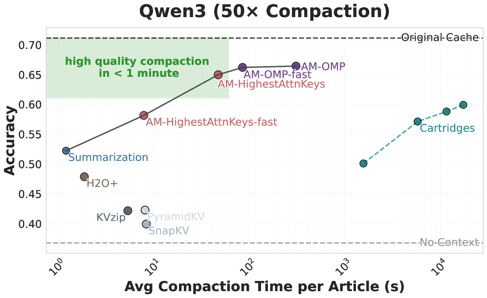</details> Figure 1: Accuracy vs. Compaction Time Trade-off (Qwen3-4B; QuALITY). We compare downstream QA accuracy ( $n=894$ ) after compaction, plotted against the average wall-clock time required to compact a context (seconds, log-scale) using a single H100 GPU at a fixed 50 $×$ compaction ratio. Our attention-matching (AM) methods trace a speed–quality tradeoff and form the Pareto frontier, outperforming prior token-selection baselines and exceeding the performance of Cartridges (Eyuboglu et al., 2025) while being 2 orders of magnitude faster; additional Cartridges training may further improve its results. Recently, Eyuboglu et al. (2025) propose Cartridges, an approach that can be interpreted as performing context compaction in latent space. Cartridges uses prefix-tuning (Li and Liang, 2021) on synthetic “self-study” data to train a compact KV cache for a given context. This enables compaction ratios as high as $50×$ on long contexts with minimal performance loss. However, its end-to-end gradient-based optimization strategy can be prohibitively expensive, often requiring several GPU-hours to train a single Cartridge for a given context. This paper describes a family of methods for fast KV compaction that can achieve Cartridges-level compaction ratios and quality while being orders of magnitude faster. Our approach is based on an Attention Matching objective: rather than training a compact KV cache end-to-end on output likelihoods, we directly optimize for compacted keys and values to reproduce the attention outputs and attention mass for every KV-head in every layer, matching these on a set of reference queries. We show that this Attention Matching objective decomposes into simple subroutines that admit closed-form solutions that are efficient to compute in practice, allowing us to avoid gradient descent entirely at compaction time. Different design choices within our framework yield a family of methods along the speed–performance frontier. Attention Matching enables compaction that is orders of magnitude faster than gradient-based optimization (e.g., minutes rather than hours), with little performance degradation at ratios up to $50×$ (see Figure ˜ 1). ## 2 KV Compaction via Attention Matching Consider the problem of compacting $T$ tokens from a context. Let $\bm{K},\bm{V}∈ℝ^T× d$ denote the corresponding keys and values for a single KV-head, where $d$ is the head dimension. Rotary embeddings are assumed to have already been applied to cached keys. KV compaction aims to replace $(\bm{K},\bm{V})$ with a shorter cache $(\bm{C}_k,\bm{C}_v)∈ℝ^t× d$ with $t<T$ such that conditioning on $(\bm{C}_k,\bm{C}_v)$ behaves similarly to conditioning on $(\bm{K},\bm{V})$ for any query $\bm{q}∈ℝ^1× d$ . A key requirement is compatibility with ordinary KV caching: compaction should remain valid even when the compacted prefix is concatenated with arbitrary uncompacted tokens (e.g., the most recent turn) or with future tokens appended after compaction (e.g., user queries or model continuations). Concretely, for any additional key–value blocks $(\bm{K}_fixed,\bm{V}_fixed)$ , we would ideally like $$ ≤ft(\bm{q};\begin{bmatrix}\bm{K}\\ \bm{K}_fixed\end{bmatrix},\begin{bmatrix}\bm{V}\\ \bm{V}_fixed\end{bmatrix}\right)≈≤ft(\bm{q};\begin{bmatrix}\bm{C}_k\\ \bm{K}_fixed\end{bmatrix},\begin{bmatrix}\bm{C}_v\\ \bm{V}_fixed\end{bmatrix}\right). $$ Written explicitly (omitting the $√{d}$ scaling for readability; see Appendix A), we would like $$ \frac{\exp≤ft(\bm{q}\begin{bmatrix}\bm{K}\\ \bm{K}_fixed\end{bmatrix}^⊤\right)\begin{bmatrix}\bm{V}\\ \bm{V}_fixed\end{bmatrix}}{∑_j=1^T+S\exp≤ft(\bm{q}\begin{bmatrix}\bm{K}\\ \bm{K}_fixed\end{bmatrix}_j^⊤\right)} ≈ \frac{\exp≤ft(\bm{q}\begin{bmatrix}\bm{C}_k\\ \bm{K}_fixed\end{bmatrix}^⊤\right)\begin{bmatrix}\bm{C}_v\\ \bm{V}_fixed\end{bmatrix}}{∑_j=1^t+S\exp≤ft(\bm{q}\begin{bmatrix}\bm{C}_k\\ \bm{K}_fixed\end{bmatrix}_j^⊤\right)}. $$ Directly enforcing this for all possible future $(\bm{K}_fixed,\bm{V}_fixed)$ is challenging. Instead, we use the fact that attention over concatenated blocks decomposes into a mixture of each block’s locally normalized attention output, weighted by that block’s attention mass. Efficient attention implementations such as FlashAttention (Dao et al., 2022) and Cascade Inference (Ye et al., 2024; Juravsky et al., 2024) exploit the same decomposition. For a key block $\bm{K}$ , define $$ Mass(\bm{q};\bm{K}) = ∑_j\exp≤ft(\bm{q}\bm{K}_j^⊤\right). $$ This suggests a sufficient compaction strategy that does not depend on unknown future tokens: over a set of reference (or “training”) queries, match (i) the compacted block’s local attention output and (ii) its attention mass. One subtlety is that with $t<T$ , exact mass matching using only $\bm{C}_k$ is impossible. For example, for $\bm{q}=\bm{0}$ we have $Mass(\bm{0};\bm{K})=T$ , whereas $Mass(\bm{0};\bm{C}_k)=t$ for any $\bm{C}_k∈ℝ^t× d$ . We therefore introduce a per-token scalar bias $\bm{β}∈ℝ^t$ , which multiplicatively reweights the contribution of each retained key to the mass. We later show that these scalar biases arise naturally in Attention Matching. Specifically, we optimize $(\bm{C}_k,\bm{β},\bm{C}_v)$ , where $\bm{C}_k,\bm{C}_v∈ℝ^t× d$ and $\bm{β}∈ℝ^t$ so that for all queries $\bm{q}$ of interest, $$ \displaystyle\frac{\exp≤ft(\bm{q}\bm{K}^⊤\right)\bm{V}}{∑_j=1^T\exp≤ft(\bm{q}\bm{K}_j^⊤\right)} \displaystyle≈\frac{\exp≤ft(\bm{q}\bm{C}_k^⊤+\bm{β}\right)\bm{C}_v}{∑_j=1^t\exp≤ft(\bm{q}(\bm{C}_k)_j^⊤+\bm{β}_j\right)}, \displaystyle∑_j=1^T\exp≤ft(\bm{q}\bm{K}_j^⊤\right) \displaystyle≈∑_j=1^t\exp≤ft(\bm{q}(\bm{C}_k)_j^⊤+\bm{β}_j\right). \tag{1} $$ Equation (1) matches the compacted block’s local attention output, while Eq. (2) matches its attention mass; together, these preserve the block’s contribution under concatenation with arbitrary fixed or future tokens (Appendix A.2). In contrast, methods that only drop or merge tokens without biases (e.g., evicting $T-t$ tokens) systematically underestimate the compacted block’s contribution during future decoding. The scalar biases add negligible memory overhead (an additional factor of $\frac{2d+1}{2d}$ ) and negligible-to-zero change in attention runtime. They are supported in common attention implementations such as PyTorch SDPA and FlexAttention (Dong et al., 2025). Finally, although the compacted cache stores only $t$ KV entries, it retains a logical length $T$ so that newly appended tokens receive the same position IDs (and thus the same RoPE phases) as they would under the uncompacted prefix. We view this as disentangling the cumulative length a cache has seen from its physical size. ## 3 Methods We now present a family of methods for constructing $(\bm{C}_k,\bm{β},\bm{C}_v)$ . Our approach is defined with respect to a set of reference queries $\bm{Q}_ref=[\bm{q}_1;…;\bm{q}_n]∈ℝ^n× d$ , which serve as a proxy for the queries the model is likely to produce when attending to the context. Jointly optimizing $(\bm{C}_k,\bm{β},\bm{C}_v)$ is computationally difficult and typically requires gradient-based optimization, which we aim to avoid at compaction time. Instead, we first construct the compacted keys $\bm{C}_k$ , then compute the bias terms $\bm{β}$ , and finally obtain $\bm{C}_v$ , all in closed form. ### 3.1 Sampling Reference Queries $\bm{Q}_\textrm{ref}$ We consider two main approaches for constructing $\bm{Q}_ref$ . #### Repeat-prefill. Following KVzip (Kim et al., 2025a), we construct a sequence $$ ``\{C\} Repeat the previous context. \{C\}'' $$ (with the model’s chat template applied appropriately), run a prefill pass on this sequence, and extract the query vectors used while the model reconstructs $C$ (i.e., query activations starting from the instruction through the second $C$ ). We found that the simpler variant of running a prefill on $C$ alone, which we call context-prefill (and used by H2O (Zhang et al., 2023)), was cheaper (see Table 1) but performed slightly worse than repeat-prefill. #### Self-study. Self-study (Eyuboglu et al., 2025) generates synthetic interactions conditioned on a fixed context $C$ . We use it as a lightweight way to broaden the query distribution: we prompt the model with $C$ and a small set of fixed prompts (e.g., “Aggregate all key facts mentioned in the context”) or model-generated conversation-starters. We then sample responses and extract the resulting query vectors. In practice, we run only four prompts (Appendix C.4), with the majority of reference queries coming from repeat-prefill. These approaches concentrate reference queries on representations the model naturally produces when processing and reasoning about $C$ . Empirically, in Appendix D, we observe that self-study yields the best downstream performance; context-prefill and repeat-prefill are nearly as good while being faster. We also find that randomly sampling $\bm{q}_i∼N(0,\bm{I}_d)$ (random-vectors) works, though it lags the other approaches. #### “On-policy” queries. Per-layer compaction can induce distribution shift in queries: compacting early layers changes the residual stream seen by later layers, so the queries they produce may differ from those extracted from the unmodified model. To reduce this mismatch, we compact layers sequentially and, for each layer $\ell$ , extract $\bm{Q}_ref^\ell$ by running the model with layers $<\ell$ already compacted, then optimize compaction at layer $\ell$ using these on-policy queries. This yields slight but consistent improvements. ### 3.2 Constructing $\bm{β}$ and $\bm{C}_v$ Before describing how we construct compact keys $\bm{C}_k$ , we first explain how we learn $\bm{β}$ and $\bm{C}_v$ to satisfy the attention-matching objectives (Eqs. 1 – 2) given reference queries $\bm{Q}_ref=[\bm{q}_1;…;\bm{q}_n]∈ℝ^n× d$ and compacted $\bm{C}_k$ . (In one of the variants we consider, we alternate between fitting subsets of $\bm{C}_k$ and $\bm{β},\bm{C}_v$ .) #### Fitting $\bm{β}$ . Let $m=[m_1,\dots,m_n]^⊤$ be the vector of original attention mass, i.e., $$ m_i=∑_k=1^T\exp(\bm{q}_i\bm{K}_k^⊤). $$ Parameterizing $w_j=\exp(\bm{β}_j)>0$ , we would then like $$ m_i≈∑_j=1^t\exp\bigl(\bm{q}_i(\bm{C}_k)_j^⊤+\bm{β}_j\bigr)=∑_j=1^tw_j\exp\bigl(\bm{q}_i(\bm{C}_k)_j^⊤\bigr). $$ This results in the following optimization problem $$ \min_w: w_j≥ 0\|\bm{A}w-m\|_2^2 $$ where $\bm{A}_ij=\exp\bigl(\bm{q}_i(\bm{C}_k)_j^⊤\bigr)$ and $w=[w_1,\dots,w_t]^⊤$ . We solve for this via nonnegative least squares (NNLS; see Appendix C.2 for implementation details), and then set $\bm{β}_j=\log(w_j)$ , clamping $w_j$ to a small positive value if needed. Intuitively, $w_j$ represents how many original keys’ worth of attention mass the compact key $(\bm{C}_k)_j$ accounts for. #### Fitting $\bm{C}_v$ . Recall that the attention-output matching condition for a query $\bm{q}$ is given by, $$ \frac{\exp(\bm{q}\bm{K}^⊤)\bm{V}}{∑_j=1^T\exp(\bm{q}\bm{K}_j^⊤)} ≈ ≤ft(\frac{\exp\bigl(\bm{q}\bm{C}_k^⊤+\bm{β}\bigr)}{∑_j=1^t\exp\bigl(\bm{q}(\bm{C}_k)_j^⊤+\bm{β}_j\bigr)}\right)\bm{C}_v $$ With $\bm{C}_k$ and $\bm{β}$ fixed, we can solve for $\bm{C}_v$ with ordinary least squares. For each reference query $\bm{q}_i$ we compute | | $\displaystyle y_i$ | $\displaystyle=\frac{\exp(\bm{q}_i\bm{K}^⊤)\bm{V}}{∑_j=1^T\exp(\bm{q}_i\bm{K}_j^⊤)}∈ℝ^1× d,$ | | | --- | --- | --- | --- | Stacking into $\bm{Y}=[y_1;\dots;y_n]∈ℝ^n× d$ and $\bm{X}=[x_1;\dots;x_n]∈ℝ^n× t$ , we solve for $\bm{C}_v$ with $$ \displaystyle\bm{C}_v^⋆ \displaystyle=\arg\min_\bm{C_v}\|\bm{X}\bm{C}_v-\bm{Y}\|_F^2, \displaystyle=(\bm{X}^⊤\bm{X})^-1\bm{X}^⊤\bm{Y}. \tag{3} $$ In summary, given any set of compacted keys $\bm{C}_k$ , simple linear-algebra routines—least squares and nonnegative least squares—allow us to learn $(\bm{β},\bm{C}_v)$ that minimize $\ell_2$ error in the attention mass and attention outputs over the reference queries. Now the main challenge becomes selecting $\bm{C}_k$ . ### 3.3 Selecting $\bm{C}_k$ We do not have a closed-form solution for constructing $\bm{C}_k$ in general. However we found it empirically effective (and efficient) to restrict $\bm{C}_k$ to be a subset of the original keys, i.e., $\bm{C}_k=\bm{K}_S,:$ for some index set $S⊂\{1,…,T\}$ with $|S|=t$ . This allows us to avoid iterative gradient-based optimization. We consider two methods for choosing this subset, which have different efficiency-performance tradeoffs. #### Highest attention keys. A simple approach in prior work on KV cache eviction/pruning (Zhang et al., 2023; Li et al., 2024; Kim et al., 2025a) is to retain keys that receive the most attention. In our setting, we measure this under the reference queries. For each reference query $\bm{q}_i$ , we compute attention weights over the original keys: $$ a_i=(\bm{q}_i\bm{K}^⊤)∈ℝ^1× T. $$ We then aggregate these weights across queries via root mean square over $(a_1,j,…,a_n,j)$ to obtain a per-key importance score $s_j$ . We found RMS to be more robust than mean or max aggregation (Appendix F.1). #### Orthogonal matching pursuit (OMP) keys. The method above is a fast and effective heuristic in practice. As a more direct alternative, we can explicitly match the attention mass using orthogonal matching pursuit (OMP; Tropp and Gilbert, 2007), which greedily builds $\bm{C}_k$ and $\bm{β}$ to best satisfy Eq. 2. Define the mass feature matrix $\bm{Φ}∈ℝ^n× T$ with $\bm{Φ}_ij=\exp(\bm{q}_i\bm{K}_j^⊤)$ and target vector $m$ with $m_i=∑_j\bm{Φ}_ij$ . We seek a sparse subset $S$ and weights $w≥ 0$ minimizing $\|\bm{Φ}_:,Sw-m\|_2^2$ . OMP selects $S$ greedily: at each step, it adds the key whose column maximally reduces the residual, then refits $w$ via NNLS (Algorithm 1). This algorithm directly yields $\bm{β}=\logw$ ; we then fit $\bm{C}_v$ via least squares as above. Algorithm 1 OMP Key Selection 0: Original keys $\bm{K}∈ℝ^T× d$ , queries $\bm{Q}∈ℝ^n× d$ , budget $t$ 0: Indices $S$ , weights $w$ (with $\bm{β}=\logw$ ) 1: $\bm{Φ}_ij←\exp(\bm{q}_i\bm{K}_j^⊤/√{d})$ {Mass feature matrix} 2: $m_i←∑_j=1^T\bm{Φ}_ij$ {Target mass vector} 3: $r←m, S←∅$ 4: for $k=1$ to $t$ do 5: $j^⋆←\arg\max_j∉ S(r^⊤\bm{Φ}_:,j)$ 6: $S← S∪\{j^⋆\}$ 7: $w←\arg\min_w≥ 0\|\bm{Φ}_:,Sw-m\|_2^2$ {NNLS} 8: $r←m-\bm{Φ}_:,Sw$ 9: end for 10: return $S,w$ While OMP performs best empirically, it is slower than the other methods: greedy selection with NNLS refitting scales at least linearly in $t$ . In practice, selecting multiple keys per step and refitting at intervals reduces compaction time by $4$ – $8×$ with little degradation (Appendix C.1). ### 3.4 Nonuniform Compaction Different attention heads can exhibit different attention patterns (Wu et al., 2025; Xiao et al., 2025; Bick et al., 2025), suggesting that a fixed compaction ratio across all heads is suboptimal. We say that uniform compaction uses the same ratio for every KV-head at every layer, whereas nonuniform compaction assigns a potentially different ratio to each head and layer. A naïve nonuniform cache implementation would pad all heads to the length of the longest KV-head, increasing the effective context length and partially negating compute savings. However, attention kernels that support variable-length sequences (e.g., FlashAttention (Dao, 2024)) can avoid this overhead by packing per-head KV segments into a flat, variable-length (varlen) representation. With such packing, nonuniform KV caches can achieve the same memory and compute benefits of a uniform cache of the same total size (Feng et al., 2025; Rehg, 2024). 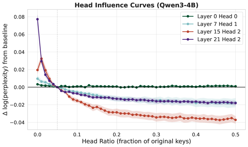To motivate a reusable nonuniform compaction schedule for each model, we first show that attention-head sensitivity is largely input-invariant—although absolute loss varies by example, the relative ranking of head importance remains stable. Figure 2 shows the resulting sensitivity curves for Qwen3-4B, averaged over contexts. These rankings also transfer across datasets; the same qualitative pattern appears on LongHealth (Appendix E). <details> <summary>x2.png Details</summary>  ### Visual Description ## Line Chart: Head Influence Curves (Qwen3-4B) ### Overview The chart visualizes the change in perplexity (Δ log(perplexity)) relative to a baseline as a function of "Head Ratio" (fraction of original keys retained). Four data series represent different layer-head combinations, with shaded regions indicating confidence intervals. ### Components/Axes - **X-axis**: Head Ratio (fraction of original keys), ranging from 0.0 to 0.5 in increments of 0.1. - **Y-axis**: Δ log(perplexity) from baseline, ranging from -0.04 to 0.08. - **Legend**: Located in the top-right corner, mapping colors to layer-head pairs: - Green: Layer 0 Head 0 - Light Blue: Layer 7 Head 1 - Red: Layer 15 Head 2 - Purple: Layer 21 Head 2 ### Detailed Analysis 1. **Layer 0 Head 0 (Green)**: - Remains nearly flat at ~0.0 across all Head Ratios. - Confidence interval is tightly clustered (~±0.002). 2. **Layer 7 Head 1 (Light Blue)**: - Starts at ~0.015 at Head Ratio 0.0, dips to ~-0.01 at 0.1, then stabilizes near -0.005. - Confidence interval widens slightly at lower Head Ratios. 3. **Layer 15 Head 2 (Red)**: - Peaks at ~0.035 at Head Ratio 0.0, drops sharply to ~-0.03 by 0.1, then stabilizes near -0.025. - Confidence interval is broadest at Head Ratio 0.0 (~±0.015). 4. **Layer 21 Head 2 (Purple)**: - Sharp peak at ~0.08 at Head Ratio 0.0, plunges to ~-0.01 by 0.1, then stabilizes near -0.005. - Confidence interval is narrowest at Head Ratio 0.0 (~±0.005). ### Key Observations - **Layer 21 Head 2** exhibits the most dramatic change, with a 0.09 drop in Δ log(perplexity) from 0.0 to 0.1 Head Ratio. - **Layer 0 Head 0** shows minimal sensitivity to Head Ratio changes. - **Layer 15 Head 2** and **Layer 21 Head 2** have the largest confidence intervals at Head Ratio 0.0, suggesting higher variability in measurements. - All lines except Layer 0 Head 0 trend downward as Head Ratio increases. ### Interpretation The data suggests that reducing the number of keys (Head Ratio < 1.0) generally decreases perplexity (improves model performance) for most layers, with higher layers (e.g., Layer 21) showing stronger effects. The stability of Layer 0 Head 0 implies it is less critical for perplexity. The sharp initial drops for Layers 15 and 21 indicate that key retention has a disproportionate impact in early stages. Confidence intervals highlight measurement uncertainty, particularly for Layer 15 Head 2 at Head Ratio 0.0. This could reflect architectural sensitivity in deeper layers or variability in key importance across attention heads. </details> Figure 2: Head sensitivity curves in Qwen3-4B. We fix all KV heads to a baseline compaction ratio of $0.05×$ and vary the compaction ratio of a single head. We report the change in loss relative to the baseline (lower is better) as a function of the varied head’s compaction ratio. Curves are averaged over $10$ QuALITY articles; shaded regions denote $±$ 1 standard error of the mean across articles. Some heads (e.g., L0H0) are largely insensitive to additional capacity, whereas others (e.g., L15H2) benefit substantially from storing more KV pairs. #### Precomputed head budgets. This stability enables us to precompute, once per model, a nonuniform compaction schedule—a per-head share of the total KV budget—that can be reused across contexts and compaction ratios. Concretely, given the per-head sensitivity curves, we solve a discrete resource allocation problem using a standard greedy exchange algorithm (Algorithm 4). Starting from a uniform allocation across heads, we iteratively swap units of KV budget between heads to minimize loss implied by the sensitivity curves. We repeat this process until no swap yields further improvement. This procedure assumes approximate separability across heads: we predict the effect of reallocating budget using single-head sensitivity curves measured with other heads held fixed. The resulting schedule is an efficient model-specific nonuniform allocation procedure that prioritizes capacity for heads most sensitive to compaction. We found this allocation to be robust across instances/datasets, and thus this procedure only needs to be performed once for a given model. A visualization of the learned head budgets is provided in Appendix E. ### 3.5 Chunked Compaction To support long contexts, we apply compaction independently to contiguous chunks of the input. Because Attention Matching can select and compact arbitrary token subsets, each chunk can be processed separately and the resulting KV caches concatenated to form a single compacted cache. We consider two implementations. In KV-based chunking, we prefill the full context, slice out the KV states corresponding to each chunk, compact them independently, and merge the compacted chunks. In text-based chunking, we instead prefill and compact each chunk in isolation, and then align the resulting keys to their original global positions via a RoPE phase shift before merging. Detailed descriptions of both variants are given in Appendix C.3. The text-based approach is an approximation because chunks are prefilled without cross-chunk interactions. In practice, we find that KV-based chunking more faithfully preserves model behavior, even when chunks are semantically independent, and therefore use it by default in all experiments, including baselines. ## 4 Results <details> <summary>x3.png Details</summary>  ### Visual Description ## Line Graphs: Accuracy vs. Compacted Size Across Datasets and Methods ### Overview The image contains six line graphs comparing the accuracy of various methods across three datasets (Qwen3-4B, Llama3-1.8B, Gemma3-12B) under two evaluation metrics: QUALITY and LongHealth. Each graph plots accuracy against compacted size (0.01 to 0.20), with methods differentiated by color. The graphs show trends in performance as models are compressed. ### Components/Axes - **X-axis**: Compacted Size (0.01, 0.02, 0.05, 0.10, 0.20) - **Y-axis**: Accuracy (0.35 to 0.80) - **Legend**: Located at the bottom center, mapping colors to methods: - Purple: AM-OMP - Red: AM-HighestAttnKeys - Green: Cartridges - Blue: Summarization (various prompts) - Gray: SnapKV - Light Gray: H2O+ - Dark Gray: PyramidKV - Blue Dotted: KVzip - Dashed Line: Original Cache - Dotted Line: No Context ### Detailed Analysis #### Qwen3-4B QUALITY - **AM-OMP (Purple)**: Starts at ~0.65 (0.01) and rises to ~0.75 (0.20), maintaining the highest accuracy. - **AM-HighestAttnKeys (Red)**: Begins at ~0.60 (0.01), peaks at ~0.72 (0.10), then plateaus. - **Cartridges (Green)**: Flat line at ~0.62 across all compacted sizes. - **Summarization (Blue)**: Starts at ~0.45 (0.01), rises to ~0.55 (0.10), then drops to ~0.50 (0.20). - **SnapKV (Gray)**: Gradual increase from ~0.40 (0.01) to ~0.55 (0.20). - **H2O+ (Light Gray)**: Starts at ~0.35 (0.01), rises to ~0.50 (0.10), then declines to ~0.45 (0.20). - **PyramidKV (Dark Gray)**: Flat at ~0.40 (0.01–0.20). - **KVzip (Blue Dotted)**: Starts at ~0.40 (0.01), peaks at ~0.55 (0.10), then drops to ~0.50 (0.20). - **Original Cache (Dashed)**: Flat at ~0.65. - **No Context (Dotted)**: Flat at ~0.35. #### Qwen3-4B LongHealth - **AM-OMP (Purple)**: Starts at ~0.60 (0.01), rises to ~0.70 (0.10), then plateaus at ~0.72 (0.20). - **AM-HighestAttnKeys (Red)**: Begins at ~0.55 (0.01), peaks at ~0.68 (0.10), then drops to ~0.65 (0.20). - **Cartridges (Green)**: Flat at ~0.65 (0.01–0.20). - **Summarization (Blue)**: Starts at ~0.35 (0.01), rises to ~0.45 (0.10), then drops to ~0.40 (0.20). - **SnapKV (Gray)**: Gradual increase from ~0.30 (0.01) to ~0.50 (0.20). - **H2O+ (Light Gray)**: Starts at ~0.30 (0.01), rises to ~0.45 (0.10), then declines to ~0.40 (0.20). - **PyramidKV (Dark Gray)**: Flat at ~0.35 (0.01–0.20). - **KVzip (Blue Dotted)**: Starts at ~0.35 (0.01), peaks at ~0.50 (0.10), then drops to ~0.45 (0.20). - **Original Cache (Dashed)**: Flat at ~0.60. - **No Context (Dotted)**: Flat at ~0.30. #### Llama3-1.8B QUALITY - **AM-OMP (Purple)**: Starts at ~0.55 (0.01), rises to ~0.65 (0.10), then plateaus at ~0.68 (0.20). - **AM-HighestAttnKeys (Red)**: Begins at ~0.50 (0.01), peaks at ~0.62 (0.10), then drops to ~0.60 (0.20). - **Cartridges (Green)**: Flat at ~0.55 (0.01–0.20). - **Summarization (Blue)**: Starts at ~0.40 (0.01), rises to ~0.50 (0.10), then drops to ~0.45 (0.20). - **SnapKV (Gray)**: Gradual increase from ~0.35 (0.01) to ~0.55 (0.20). - **H2O+ (Light Gray)**: Starts at ~0.30 (0.01), rises to ~0.45 (0.10), then declines to ~0.40 (0.20). - **PyramidKV (Dark Gray)**: Flat at ~0.35 (0.01–0.20). - **KVzip (Blue Dotted)**: Starts at ~0.40 (0.01), peaks at ~0.50 (0.10), then drops to ~0.45 (0.20). - **Original Cache (Dashed)**: Flat at ~0.60. - **No Context (Dotted)**: Flat at ~0.35. #### Llama3-1.8B LongHealth - **AM-OMP (Purple)**: Starts at ~0.50 (0.01), rises to ~0.60 (0.10), then plateaus at ~0.62 (0.20). - **AM-HighestAttnKeys (Red)**: Begins at ~0.45 (0.01), peaks at ~0.60 (0.10), then drops to ~0.58 (0.20). - **Cartridges (Green)**: Flat at ~0.55 (0.01–0.20). - **Summarization (Blue)**: Starts at ~0.30 (0.01), rises to ~0.40 (0.10), then drops to ~0.35 (0.20). - **SnapKV (Gray)**: Gradual increase from ~0.25 (0.01) to ~0.45 (0.20). - **H2O+ (Light Gray)**: Starts at ~0.25 (0.01), rises to ~0.40 (0.10), then declines to ~0.35 (0.20). - **PyramidKV (Dark Gray)**: Flat at ~0.30 (0.01–0.20). - **KVzip (Blue Dotted)**: Starts at ~0.30 (0.01), peaks at ~0.45 (0.10), then drops to ~0.40 (0.20). - **Original Cache (Dashed)**: Flat at ~0.55. - **No Context (Dotted)**: Flat at ~0.25. #### Gemma3-12B QUALITY - **AM-OMP (Purple)**: Starts at ~0.60 (0.01), rises to ~0.70 (0.10), then plateaus at ~0.72 (0.20). - **AM-HighestAttnKeys (Red)**: Begins at ~0.55 (0.01), peaks at ~0.68 (0.10), then drops to ~0.65 (0.20). - **Cartridges (Green)**: Flat at ~0.58 (0.01–0.20). - **Summarization (Blue)**: Starts at ~0.45 (0.01), rises to ~0.55 (0.10), then drops to ~0.50 (0.20). - **SnapKV (Gray)**: Gradual increase from ~0.40 (0.01) to ~0.55 (0.20). - **H2O+ (Light Gray)**: Starts at ~0.35 (0.01), rises to ~0.50 (0.10), then declines to ~0.45 (0.20). - **PyramidKV (Dark Gray)**: Flat at ~0.40 (0.01–0.20). - **KVzip (Blue Dotted)**: Starts at ~0.45 (0.01), peaks at ~0.55 (0.10), then drops to ~0.50 (0.20). - **Original Cache (Dashed)**: Flat at ~0.65. - **No Context (Dotted)**: Flat at ~0.35. #### Gemma3-12B LongHealth - **AM-OMP (Purple)**: Starts at ~0.55 (0.01), rises to ~0.65 (0.10), then plateaus at ~0.68 (0.20). - **AM-HighestAttnKeys (Red)**: Begins at ~0.50 (0.01), peaks at ~0.65 (0.10), then drops to ~0.62 (0.20). - **Cartridges (Green)**: Flat at ~0.58 (0.01–0.20). - **Summarization (Blue)**: Starts at ~0.40 (0.01), rises to ~0.50 (0.10), then drops to ~0.45 (0.20). - **SnapKV (Gray)**: Gradual increase from ~0.35 (0.01) to ~0.50 (0.20). - **H2O+ (Light Gray)**: Starts at ~0.30 (0.01), rises to ~0.45 (0.10), then declines to ~0.40 (0.20). - **PyramidKV (Dark Gray)**: Flat at ~0.35 (0.01–0.20). - **KVzip (Blue Dotted)**: Starts at ~0.40 (0.01), peaks at ~0.50 (0.10), then drops to ~0.45 (0.20). - **Original Cache (Dashed)**: Flat at ~0.60. - **No Context (Dotted)**: Flat at ~0.30. ### Key Observations 1. **AM-OMP** consistently outperforms other methods across all datasets and metrics, maintaining the highest accuracy as compacted size increases. 2. **AM-HighestAttnKeys** shows strong performance but declines at larger compacted sizes (e.g., 0.20). 3. **Cartridges** maintains stable but suboptimal accuracy compared to AM-OMP. 4. **Summarization** methods exhibit a "U-shaped" trend, peaking at mid-compacted sizes before declining. 5. **SnapKV** and **H2O+** show gradual improvement but lag behind AM-OMP. 6. **PyramidKV** and **KVzip** underperform, with flat or declining trends. 7. **Original Cache** (dashed line) serves as a baseline, outperforming most methods except AM-OMP. 8. **No Context** (dotted line) consistently has the lowest accuracy. ### Interpretation The data suggests that **AM-OMP** is the most robust method for maintaining accuracy under compression, likely due to its adaptive optimization. Methods like **AM-HighestAttnKeys** and **Cartridges** offer trade-offs between compression and performance, while **Summarization** and **KVzip** struggle with larger compacted sizes. The **Original Cache** baseline highlights the importance of context retention, as "No Context" methods fail to retain meaningful accuracy. The decline in performance at larger compacted sizes (e.g., 0.20) across most methods indicates a critical threshold where compression harms utility. This analysis is critical for optimizing model deployment in resource-constrained environments. 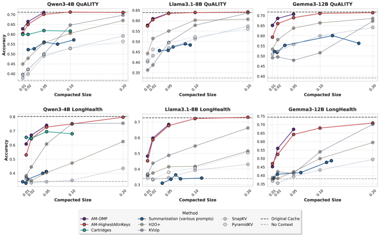</details> Figure 3: Accuracy vs. compaction ratio across methods. We compare AM-OMP and AM-HighestAttentionKeys against Cartridges, summarization, and four prior methods. Evaluations are conducted on QuALITY and LongHealth using Qwen3-4B, Llama3.1-8B, and Gemma3-12B. Attention Matching (AM) consistently outperforms other approaches across compaction ratios, while matching Cartridges’ performance at ultra-high compaction. We evaluate Attention Matching across a range of compaction strategies, measuring downstream quality and compaction efficiency on long-context benchmarks. #### Compared Variants. We evaluate four representative compaction variants that trade off compaction time and downstream quality by varying how reference queries are obtained and how keys are selected. The variants are ordered by performance: - AM-OMP: On-policy $\bm{Q}_ref$ from self-study + repeat-prefill; fit $(\bm{C}_k,\bm{β})$ jointly via OMP; fit $\bm{C}_v$ by least squares. - AM-OMP-fast: Same as AM-OMP, but with OMP speedups ( $k=4$ keys selected per iteration, $τ=2$ iterations between NNLS refits; Appendix C.1). - AM-HighestAttnKeys: On-policy $\bm{Q}_ref$ from self-study + repeat-prefill; select $\bm{C}_k$ by highest attention; fit $\bm{β}$ via NNLS; fit $\bm{C}_v$ by least squares. - AM-HighestAttnKeys-fast: Same as AM-HighestAttnKeys, but with $\bm{Q}_ref$ coming only from repeat-prefill. With self-study + repeat-prefill, we use at most $50{,}000$ reference queries per KV-head for each context/chunk. Importantly, this does not require a large number of generated tokens: under GQA, each token yields multiple query vectors per KV-head, and the majority of reference queries are obtained via repeat-prefill rather than self-study. On QuALITY, we generate on average approximately $5$ k self-study tokens and $7$ k repeat-prefill tokens per context. #### Baselines. We compare against (i) Cartridges (Eyuboglu et al., 2025), which performs end-to-end gradient-based optimization of a compact latent KV cache for each context; (ii) baselines based on token pruning using attention scores (H2O (Zhang et al., 2023), SnapKV (Li et al., 2024), PyramidKV (Cai et al., 2025), KVzip (Kim et al., 2025a)), instantiated in our one-shot, question-agnostic setting as described in Appendix B.3; and (iii) summarization, which replaces the original context with a shorter textual summary, either produced for the full document or by summarizing chunks and concatenating the summaries (Table 5). #### Evaluation protocol. We evaluate on QuALITY (Pang et al., 2022), a long-document comprehension benchmark (5–8k tokens; 15–20 questions per context), and LongHealth (Adams et al., 2024), a highly information-dense patient-records QA task (60k tokens per context; 100 questions per context, where each context aggregates 5 patients; 4 contexts total). See Appendix B.2 for a sample context and question. For each context, we compact once and then answer all associated multiple-choice questions by decoding from the compacted cache. For all methods, we keep the chat template tokens fixed during compaction (e.g., BOS / system-prefix tokens, which can act as attention sinks (Xiao et al., 2024)) and re-attach them after compaction. We report the compacted size $t/T$ with respect to the $T$ article tokens, excluding chat-template tokens. While we found our method is robust to compacting these template tokens, we fix them for a fair comparison with baselines. We apply KV-based chunked compaction on LongHealth with $5$ chunks for all methods except for Cartridges. Our QuALITY evaluation is done over $50$ contexts. Since evaluating Cartridges was computationally expensive, we only evaluate it on Qwen, on a fixed 20-context subset selected a priori; scores on this subset showed little deviation from the full set of 50 (Appendix B.2). ### 4.1 Main Results We first analyze the trade-off between compaction time and downstream accuracy. Figure 1 plots this for Qwen3-4B on QuALITY at a fixed $50×$ ratio. (See Figure 10 in the appendix for perplexity results.) Our Attention Matching (AM) methods trace the Pareto frontier and bridge the gap between fast heuristic baselines (e.g., summarization, H2O+, KVzip), which degrade significantly at this ratio, and optimization-heavy methods like Cartridges. In Figure 3, we sweep the compaction ratio across $3$ models on QuALITY and LongHealth. We observe that Attention Matching methods consistently outperform token-eviction baselines and summarization, particularly in the high-compaction regime ( $20×$ – $100×$ ). Performance degrades faster on LongHealth, which is highly information-dense (Appendix B.2). Summarization does particularly poorly on this dataset, matching the no-context baseline. KVzip sometimes matches Attention Matching performance, which we attribute to its non-uniform budget outperforming our precomputed budget at certain compaction ratios. ### 4.2 Sliding Window Attention The effectiveness of nonuniform compaction schedules gives some insight into why hybrid architectures with sliding-window attention (Child et al., 2019; Beltagy et al., 2020) and only a few global layers can retain much of the performance of full-attention models: even when trained with full attention, many KV-heads naturally specialize to modeling local context, while only a small number of globally attending heads capture the long-range dependencies. Does this imply that compaction is less effective for these hybrid models? To verify that our improvements still hold on sliding-window models, we evaluate Gemma-3-12B, which has an aggressive 5:1 ratio of sliding-window layers to global layers. We compact only the global-attention layers, leaving the sliding-window layers unchanged. Accordingly, the reported compaction ratios are computed over only the global-attention portion of the KV cache. As shown in Figure 3, we require only slightly more conservative compaction ratios compared to the two full-attention models. ### 4.3 Compaction Efficiency We profile the wall-clock compute cost of each component of our method on a 60k-token LongHealth context using Gemma-3-12B (64 full-attention KV heads; head dimension $d_head{=}256$ ); see Table 1). All timings are measured on a single H200 GPU. We compute compacted keys and values in FP32 and then cast to BF16 for storage; we do not experiment with quantization in this work. | Stage | Method | Time (s) | | --- | --- | --- | | context-prefill | 7 | | | Query generation | repeat-prefill | 8 | | self-study | 139 | | | Highest attention | 3 | | | Key selection | OMP | 565 | | OMP-fast ( $k{=}4$ , refit interval=2) | 104 | | | $\bm{β}$ fitting | NNLS | 2.2 | | Value fitting | Least squares | 1.8 | Table 1: Wall-clock compaction time breakdown on a 60k-token LongHealth context with Gemma-3-12B on a single H200 GPU. Query generation dominates runtime in this long-context setting and can likely be substantially optimized. All results here use a single GPU and self-study/repeat-prefill with chunked prefill with chunk size 4096. Although we only evaluate models up to 12B parameters, we note that KV cache size varies quite little across different size variants of open-source models. For example, for the same sequence length, Qwen3-235B-A22B yields a KV cache only $∼$ 30% larger than Qwen3-4B (96,256 vs. 73,728 elements per token). We therefore expect our compaction efficiency results to scale without much additional cost to much larger mixture of expert models commonly used in deployment. ### 4.4 Extension: Summarization plus Attention Matching While summarization rapidly degrades performance on tasks that require extracting knowledge and reasoning across long contexts (Section 4.1), it may be acceptable in cases where not all prior information needs to be retained (for example, when there exist retrieval or search mechanisms), or for filtering out noise or hallucinations. In Table 2, we demonstrate that Attention Matching works on top of summarization: applying AM-OMP to summarized text achieves $200×$ compaction (6340 $→$ 31 effective tokens on average) with performance comparable to summarization alone, which in our case provides only $∼ 20×$ compaction. | Full Context Summarize Summarize × (0.2× AM-OMP) | 100.00 4.80 0.92 | 71.5 55.2 55.7 | | --- | --- | --- | | Summarize × (0.1× AM-OMP) | 0.46 | 55.0 | | Summarize × (0.05× AM-OMP) | 0.21 | 49.2 | Table 2: Summarization plus Attention Matching. Applying AM-OMP on top of a summary enables up to $∼$ 200 $×$ total compaction with accuracy comparable to summarization alone. 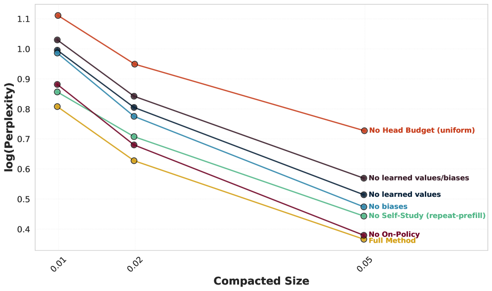### 4.5 Ablations We’ve introduced several concepts: post-compaction attention biases, fitted values, nonuniform head budgets, and query-sampling methods. In Figure 4, we leave out components of our main AM-OMP method and measure loss on reference generations. We see that every component is necessary to achieve the best results, with the least important being the use of self-study and the use of on-policy queries, and the most important being nonuniform head budgets. We note that omitting attention biases and retaining the original values for selected keys still yields a reasonable approximation. However, refitting $\bm{β}$ and $\bm{C}_v$ via (nonnegative) least squares better aligns with our objective of approximating the original cache, adds little overhead, and consistently improves performance. ## 5 Related Work While some prior works approach KV cache reduction as a per-token online problem—continuously evicting or merging tokens at each decoding step to maintain a fixed state size (e.g., Zhang et al., 2023; Oren et al., 2024) —we study compaction as a one-shot operation applied at the moment a context becomes too large. Methods in this setting are able to make globally informed decisions over the full prefix. Moreover, one-shot compaction can be applied repeatedly to maintain a fixed maximum state size, as in Appendix F.3. <details> <summary>x4.png Details</summary>  ### Visual Description ## Line Chart: log(Perplexity) vs Compacted Size ### Overview The chart visualizes the relationship between **log(Perplexity)** (y-axis) and **Compacted Size** (x-axis) for seven different methods. Each line represents a method's performance across three compacted size values: 0.01, 0.02, and 0.05. Perplexity decreases as compacted size increases for all methods, but the rate and magnitude of reduction vary. --- ### Components/Axes - **X-axis (Compacted Size)**: Logarithmic scale with ticks at 0.01, 0.02, and 0.05. - **Y-axis (log(Perplexity))**: Logarithmic scale ranging from 0.4 to 1.1. - **Legend**: Positioned on the right, with seven color-coded lines: 1. **Orange**: No Head Budget (uniform) 2. **Dark Red**: No learned values/biases 3. **Dark Blue**: No learned values 4. **Light Blue**: No biases 5. **Green**: No Self-Study (repeat-prefill) 6. **Maroon**: No On-Policy 7. **Yellow**: Full Method --- ### Detailed Analysis 1. **No Head Budget (uniform)** (Orange): - Starts at **1.1** (x=0.01) and decreases to **0.72** (x=0.05). - Steepest decline among all methods. 2. **No learned values/biases** (Dark Red): - Begins at **1.03** (x=0.01) and drops to **0.57** (x=0.05). - Consistent downward trend. 3. **No learned values** (Dark Blue): - Starts at **0.99** (x=0.01) and falls to **0.52** (x=0.05). - Slightly less steep than "No learned values/biases." 4. **No biases** (Light Blue): - Begins at **0.99** (x=0.01) and decreases to **0.48** (x=0.05). - Moderate decline. 5. **No Self-Study (repeat-prefill)** (Green): - Starts at **0.86** (x=0.01) and drops to **0.45** (x=0.05). - Steady reduction. 6. **No On-Policy** (Maroon): - Begins at **0.88** (x=0.01) and falls to **0.39** (x=0.05). - Sharp decline, second only to "Full Method." 7. **Full Method** (Yellow): - Starts at **0.81** (x=0.01) and decreases to **0.38** (x=0.05). - Most effective at reducing perplexity. --- ### Key Observations - **Highest Perplexity**: "No Head Budget (uniform)" consistently has the highest perplexity across all compacted sizes. - **Lowest Perplexity**: "Full Method" achieves the lowest perplexity at all sizes. - **Trend**: All methods show decreasing perplexity as compacted size increases, but the "Full Method" outperforms others significantly. - **Outlier**: "No Head Budget (uniform)" maintains the highest perplexity even at the largest compacted size (0.05). --- ### Interpretation The data suggests that the **Full Method** is the most effective at minimizing perplexity, likely due to its comprehensive approach (retaining learned values, biases, and on-policy data). In contrast, the **No Head Budget (uniform)** method performs worst, indicating that uniform head budgets without learned components are suboptimal. The logarithmic scale emphasizes relative differences, showing that even small reductions in perplexity (e.g., from 0.81 to 0.38 for the Full Method) represent substantial improvements. The trends highlight the importance of retaining learned values and biases in reducing model uncertainty. </details> Figure 4: Leave-one-out experiments. We ablate our main AM-OMP method and measure average log-perplexity of generations decoded from the original cache, since this is lower in variance and well-correlated with downstream performance (Appendix F.2). In “no biases,” we first compute OMP as usual and then zero out $\bm{β}$ , keeping the keys selected by OMP. Token-space approaches to handling long context generally involve combinations of retrieval-augmented generation (Lewis et al., 2020), context compaction via summarization or token dropping (Jiang et al., 2023; Li et al., 2023; Anthropic, 2025), and agentic memory management (Packer et al., 2024; Zhang et al., 2025). These approaches are largely orthogonal to latent-space compaction. While summarization rapidly degrades performance on tasks that require extracting knowledge and reasoning across long contexts (Section 4), it may be acceptable in cases where not all prior information needs to be retained (for instance, when there exist retrieval or search mechanisms). The two approaches can be combined with strong performance (Table 2); the most effective memory system may have a mix of retrieval and compaction in both token-space and latent-space. In addition to the baselines that we evaluate (Zhang et al., 2023; Li et al., 2024; Cai et al., 2025; Kim et al., 2025a), a large body of other work explores token-merging (Wang et al., 2024; Zhang et al., 2024; Liu et al., 2025; Wan et al., 2025) and token-eviction (Oren et al., 2024; Ge et al., 2024; Tang et al., 2024; Chari and Durme, 2025; Łańcucki et al., 2025). The KVPress (Devoto et al., 2025) repository benchmarks over $20$ such methods; we include the top-performing approach, KVzip (Kim et al., 2025a), among our baselines. One line of prior work explores having models generate a set of soft tokens or “gist” tokens (Bulatov et al., 2022; Chevalier et al., 2023; Mu et al., 2023) that can be used to replace the original cache. These methods require training or finetuning the model to produce such representations, whereas our approach operates as a post-hoc procedure on any pretrained model without modification. Our work is also related to Lexico (Kim et al., 2025b), which compresses keys and values by learning a universal dictionary per layer and uses orthogonal matching pursuit (OMP) at inference time to store each per-token key/value vector as a sparse code over the learned atoms. Lexico’s objective is $\ell_2$ reconstruction of KV vectors whereas we optimize compacted KV vectors for matching attention behavior. DuoAttention (Xiao et al., 2025) proposes that attention heads be split into a small set of retrieval heads that use a full-length KV cache, and streaming heads that can run with a constant-length cache containing only attention sinks and recent tokens; they learn this partition via gradient optimization over per-head gates that blend full vs. streaming attention on synthetic data, then binarize the gates for deployment. Our nonuniform compaction shares the insight that heads vary in their sensitivity to KV capacity, but we learn continuous per-head budgets via sensitivity curves and compact all heads to varying degrees. The notion of adding a per-token scalar attention bias was suggested in T5 (Raffel et al., 2020) and ALiBi (Press et al., 2022) as a form of positional encoding. Our method also employs attention biases, but for a different purpose: to correct for the attention mass received by the compacted cache. ## 6 Discussion Disentangling logical KV length from physical cache size yields a practical primitive operation: KV compaction, which can be invoked on arbitrary portions of context whenever a sequence grows too large. Attention Matching is a natural paradigm for KV compaction because it approximately preserves the two ingredients that determine a block’s contribution under concatenation—attention outputs and attention mass. Moreover, Attention Matching enables efficient algorithms for finding compact keys and values. Our work still has several limitations. For one, while our approach is orders of magnitude faster than end-to-end gradient-based methods (i.e., Cartridges), our unoptimized OMP + self-study variants still required several minutes for compaction. And while our approach outperforms Cartridges in terms of accuracy at $50×$ compaction rates, Cartridges outperforms our approach at more extreme ( $100×$ ) compaction rates on some benchmarks (LongHealth). We attribute this to the fact that gradient-based optimization can search over a wider space of compact representations—in particular, it is not restricted to optimizing intermediate attention outputs or selecting keys from the original cache—which becomes increasingly important as the compaction budget shrinks. #### Future work. Beyond speeding up query-generation or OMP-style selection, a promising direction is to move away from subset selection for $\bm{C}_k$ (e.g., directly optimizing compact keys). Another interesting direction is architectures or training procedures that support compaction as a simple primitive, or explicitly operate over a fixed set of keys and values. Integrating KV compaction into inference engines (e.g., RadixAttention-style prefix caching, varlen KV packing, and disaggregated compaction) and combining token-space retrieval/summarization with latent-space compaction are important systems directions that still require significant effort. Finally, while our experiments focus on one-shot compaction of a fixed context, the problem of maintaining memory over long-horizon interactions is another very natural setting for KV compaction. A promising application is online compaction, where we compact the KV cache mid-trajectory to support arbitrarily long-horizon generation under a fixed physical memory budget. Appendix F.3 provides a preliminary result showing that repeated context compaction via Attention Matching preserves reasoning performance on AIME. This is especially promising for long-horizon agentic settings such as coding agents, where tool call outputs and execution traces can take up a significant amount of context. Online latent compaction could be a principled alternative or complement to turn-dropping and summarization. ## 7 Conclusion We study Attention Matching as an objective for fast latent-space compaction. Our methods significantly improve the Pareto frontier of compaction cost versus quality. ## Acknowledgements We would like to thank Ani Nrusimha, Alicia Li, Sabri Eyuboglu, Zifan Wang, Jyo Pari, Oliver Sieberling, and Tarushii Goel for their valuable discussions and feedback. This work was supported by the National Science Foundation under CAREER Award No. 2441872 and MIT-IBM Watson AI Lab. This research was partly supported by the Prof. JCR Licklider Endowed UROP Fund for MIT UROP research. ## References - L. Adams, F. Busch, T. Han, J. Excoffier, M. Ortala, A. Löser, H. JWL. Aerts, J. N. Kather, D. Truhn, and K. Bressem (2024) LongHealth: a question answering benchmark with long clinical documents. External Links: 2401.14490, Link Cited by: §B.2, §4. - Anthropic (2025) Effective context engineering for AI agents. External Links: Link Cited by: §1, §5. - I. Beltagy, M. E. Peters, and A. Cohan (2020) Longformer: the long-document transformer. External Links: 2004.05150, Link Cited by: §4.2. - A. Bick, E. P. Xing, and A. Gu (2025) Understanding the skill gap in recurrent models: The role of the Gather-and-Aggregate mechanism. In Forty-second International Conference on Machine Learning, External Links: Link Cited by: §3.4. - M. Braverman, X. Chen, S. Kakade, K. Narasimhan, C. Zhang, and Y. Zhang (2020) Calibration, entropy rates, and memory in language models. In Proceedings of the 37th International Conference on Machine Learning, Cited by: §F.2. - A. Bulatov, Y. Kuratov, and M. Burtsev (2022) Recurrent memory transformer. In Advances in Neural Information Processing Systems, External Links: Link Cited by: §5. - Z. Cai, Y. Zhang, B. Gao, Y. Liu, Y. Li, T. Liu, K. Lu, W. Xiong, Y. Dong, J. Hu, and W. Xiao (2025) PyramidKV: Dynamic KV cache compression based on pyramidal information funneling. In Second Conference on Language Modeling, External Links: Link Cited by: §B.3, Figure 8, Figure 8, §4, §5. - S. Cao, G. Valiant, and P. Liang (2025) On the entropy calibration of language models. In The Thirty-ninth Annual Conference on Neural Information Processing Systems, External Links: Link Cited by: §F.2. - V. Chari and B. V. Durme (2025) Compactor: Calibrated query-agnostic KV cache compression with approximate leverage scores. External Links: 2507.08143, Link Cited by: §5. - A. Chevalier, A. Wettig, A. Ajith, and D. Chen (2023) Adapting language models to compress contexts. In Proceedings of the 2023 Conference on Empirical Methods in Natural Language Processing, External Links: Link Cited by: §5. - R. Child, S. Gray, A. Radford, and I. Sutskever (2019) Generating long sequences with sparse transformers. External Links: 1904.10509, Link Cited by: §4.2. - T. Dao, D. Fu, S. Ermon, A. Rudra, and C. Ré (2022) FlashAttention: fast and memory-efficient exact attention with IO-awareness. In Advances in Neural Information Processing Systems, External Links: Link Cited by: footnote 2. - T. Dao (2024) FlashAttention-2: faster attention with better parallelism and work partitioning. In The Twelfth International Conference on Learning Representations, External Links: Link Cited by: footnote 3. - A. Devoto, M. Jeblick, and S. Jégou (2025) Expected Attention: KV cache compression by estimating attention from future queries distribution. arXiv preprint arXiv:2510.00636. External Links: Link Cited by: §5. - J. Dong, B. Feng, D. Guessous, Y. Liang, and H. He (2025) FlexAttention: a programming model for generating fused attention variants.. In Eighth Conference on Machine Learning and Systems, External Links: Link Cited by: §2. - S. Eyuboglu, R. Ehrlich, S. Arora, N. Guha, D. Zinsley, E. Liu, W. Tennien, A. Rudra, J. Zou, A. Mirhoseini, and C. Re (2025) Cartridges: Lightweight and general-purpose long context representations via self-study. External Links: 2506.06266, Link Cited by: §B.2, §B.3, Figure 1, Figure 1, §1, §3.1, §4, Fast KV Compaction via Attention Matching. - Y. Feng, J. Lv, Y. Cao, X. Xie, and S. K. Zhou (2025) Ada-KV: optimizing KV cache eviction by adaptive budget allocation for efficient LLM inference. In The Thirty-ninth Annual Conference on Neural Information Processing Systems, External Links: Link Cited by: footnote 3. - S. Ge, Y. Zhang, L. Liu, M. Zhang, J. Han, and J. Gao (2024) Model tells you what to discard: adaptive KV cache compression for LLMs. In The Twelfth International Conference on Learning Representations, External Links: Link Cited by: §5. - Gemma Team (2025) Gemma 3 technical report. External Links: 2503.19786, Link Cited by: §B.1. - H. Jiang, Q. Wu, C. Lin, Y. Yang, and L. Qiu (2023) LLMLingua: Compressing prompts for accelerated inference of large language models. In Proceedings of the 2023 Conference on Empirical Methods in Natural Language Processing, External Links: Link Cited by: §5. - J. Juravsky, B. Brown, R. S. Ehrlich, D. Y. Fu, C. Re, and A. Mirhoseini (2024) Hydragen: high-throughput LLM inference with shared prefixes. In Workshop on Efficient Systems for Foundation Models II @ ICML2024, External Links: Link Cited by: footnote 2. - J. Kim, J. Kim, S. Kwon, J. W. Lee, S. Yun, and H. O. Song (2025a) KVzip: Query-agnostic KV cache compression with context reconstruction. In The Thirty-ninth Annual Conference on Neural Information Processing Systems, External Links: Link Cited by: §B.3, Appendix E, §1, §3.1, §3.3, §4, §5. - J. Kim, J. Park, J. Cho, and D. Papailiopoulos (2025b) Lexico: extreme KV cache compression via sparse coding over universal dictionaries. In Forty-second International Conference on Machine Learning, External Links: Link Cited by: §5. - W. Kwon, Z. Li, S. Zhuang, Y. Sheng, L. Zheng, C. H. Yu, J. E. Gonzalez, H. Zhang, and I. Stoica (2023) Efficient memory management for large language model serving with PagedAttention. In Proceedings of the ACM SIGOPS 29th Symposium on Operating Systems Principles, Cited by: §C.4. - A. Łańcucki, K. Staniszewski, P. Nawrot, and E. Ponti (2025) Inference-time hyper-scaling with KV cache compression. In The Thirty-ninth Annual Conference on Neural Information Processing Systems, External Links: Link Cited by: §5. - P. Lewis, E. Perez, A. Piktus, F. Petroni, V. Karpukhin, N. Goyal, H. Küttler, M. Lewis, W. Yih, T. Rocktäschel, S. Riedel, and D. Kiela (2020) Retrieval-augmented generation for knowledge-intensive NLP tasks. In Advances in Neural Information Processing Systems, External Links: Link Cited by: §5. - X. L. Li and P. Liang (2021) Prefix-Tuning: Optimizing continuous prompts for generation. In Proceedings of the 59th Annual Meeting of the Association for Computational Linguistics and the 11th International Joint Conference on Natural Language Processing, External Links: Link Cited by: §1. - Y. Li, B. Dong, F. Guerin, and C. Lin (2023) Compressing context to enhance inference efficiency of large language models. In Proceedings of the 2023 Conference on Empirical Methods in Natural Language Processing, External Links: Link Cited by: §5. - Y. Li, Y. Huang, B. Yang, B. Venkitesh, A. Locatelli, H. Ye, T. Cai, P. Lewis, and D. Chen (2024) SnapKV: LLM knows what you are looking for before generation. In Advances in Neural Information Processing Systems, External Links: Link Cited by: §B.3, §1, §3.3, §4, §5. - X. Liu, X. Wang, P. Liu, and G. Tang (2025) ZSMerge: zero-shot KV cache compression for memory-efficient long-context LLMs. External Links: 2503.10714, Link Cited by: §5. - Llama Team (2024) The Llama 3 herd of models. External Links: 2407.21783, Link Cited by: §B.1. - J. Mu, X. Li, and N. Goodman (2023) Learning to compress prompts with gist tokens. In Advances in Neural Information Processing Systems, External Links: Link Cited by: §5. - N. Muennighoff, Z. Yang, W. Shi, X. L. Li, L. Fei-Fei, H. Hajishirzi, L. Zettlemoyer, P. Liang, E. Candes, and T. Hashimoto (2025) S1: simple test-time scaling. In Proceedings of the 2025 Conference on Empirical Methods in Natural Language Processing, External Links: Link Cited by: §F.3. - OpenAI (2025) Context engineering - short-term memory management with sessions from OpenAI agents SDK. OpenAI. Note: OpenAI Cookbook. Page author: Emre Okcular. External Links: Link Cited by: §1. - M. Oren, M. Hassid, N. Yarden, Y. Adi, and R. Schwartz (2024) Transformers are multi-state RNNs. In Proceedings of the 2024 Conference on Empirical Methods in Natural Language Processing, External Links: Link Cited by: §5, §5. - C. Packer, S. Wooders, K. Lin, V. Fang, S. G. Patil, I. Stoica, and J. E. Gonzalez (2024) MemGPT: towards LLMs as operating systems. External Links: 2310.08560, Link Cited by: §5. - R. Y. Pang, A. Parrish, N. Joshi, N. Nangia, J. Phang, A. Chen, V. Padmakumar, J. Ma, J. Thompson, H. He, and S. Bowman (2022) QuALITY: question answering with long input texts, yes!. In Proceedings of the 2022 Conference of the North American Chapter of the Association for Computational Linguistics: Human Language Technologies, External Links: Link Cited by: §B.2, §4. - O. Press, N. Smith, and M. Lewis (2022) Train short, test long: Attention with linear biases enables input length extrapolation. In International Conference on Learning Representations, External Links: Link Cited by: §5. - Qwen Team (2025) Qwen3 technical report. External Links: 2505.09388, Link Cited by: §B.1. - C. Raffel, N. Shazeer, A. Roberts, K. Lee, S. Narang, M. Matena, Y. Zhou, W. Li, and P. J. Liu (2020) Exploring the limits of transfer learning with a unified text-to-text transformer. Journal of Machine Learning Research. External Links: Link Cited by: §5. - I. Rehg (2024) KV-Compress: Paged KV-cache compression with variable compression rates per attention head. External Links: 2410.00161, Link Cited by: footnote 3. - J. Tang, Y. Zhao, K. Zhu, G. Xiao, B. Kasikci, and S. Han (2024) QUEST: query-aware sparsity for efficient long-context LLM inference. In Proceedings of the 41st International Conference on Machine Learning, Cited by: §5. - J. A. Tropp and A. C. Gilbert (2007) Signal recovery from random measurements via orthogonal matching pursuit. IEEE Transactions on information theory 53 (12), pp. 4655–4666. Cited by: §3.3. - Z. Wan, X. Wu, Y. Zhang, Y. Xin, C. Tao, Z. Zhu, X. Wang, S. Luo, J. Xiong, L. Wang, and M. Zhang (2025) D2O: Dynamic discriminative operations for efficient long-context inference of large language models. In The Thirteenth International Conference on Learning Representations, External Links: Link Cited by: §5. - Z. Wang, B. Jin, Z. Yu, and M. Zhang (2024) Model tells you where to merge: Adaptive KV cache merging for LLMs on long-context tasks. External Links: 2407.08454, Link Cited by: §1, §5. - W. Wu, Y. Wang, G. Xiao, H. Peng, and Y. Fu (2025) Retrieval head mechanistically explains long-context factuality. In The Thirteenth International Conference on Learning Representations, External Links: Link Cited by: §3.4. - G. Xiao, J. Tang, J. Zuo, junxian guo, S. Yang, H. Tang, Y. Fu, and S. Han (2025) DuoAttention: efficient long-context LLM inference with retrieval and streaming heads. In The Thirteenth International Conference on Learning Representations, External Links: Link Cited by: §B.3, §1, §3.4, §5. - G. Xiao, Y. Tian, B. Chen, S. Han, and M. Lewis (2024) Efficient streaming language models with attention sinks. In The Twelfth International Conference on Learning Representations, External Links: Link Cited by: §1, §4. - Z. Ye, R. Lai, B. Lu, C. Lin, S. Zheng, L. Chen, T. Chen, and L. Ceze (2024) Cascade Inference: Memory bandwidth efficient shared prefix batch decoding. External Links: Link Cited by: footnote 2. - A. L. Zhang, T. Kraska, and O. Khattab (2025) Recursive language models. External Links: 2512.24601, Link Cited by: §5. - Y. Zhang, Y. Du, G. Luo, Y. Zhong, Z. Zhang, S. Liu, and R. Ji (2024) CaM: cache merging for memory-efficient LLMs inference. In Proceedings of the 41st International Conference on Machine Learning, External Links: Link Cited by: §1, §5. - Z. Zhang, Y. Sheng, T. Zhou, T. Chen, L. Zheng, R. Cai, Z. Song, Y. Tian, C. Ré, C. Barrett, Z. ". Wang, and B. Chen (2023) H2O: Heavy-Hitter Oracle for efficient generative inference of large language models. In Advances in Neural Information Processing Systems, External Links: Link Cited by: §B.3, §1, §3.1, §3.3, §4, §5, §5. ## Appendix A Attention Matching Details This appendix restates the attention-matching objectives from Section 2 in more detail. ### A.1 Notation Fix a single layer and KV-head with head dimension $d$ . Let the original keys and values be $$ \bm{K}∈ℝ^T× d, \bm{V}∈ℝ^T× d, $$ and let the compacted keys, values, and per-token bias be $$ \bm{C}_k∈ℝ^t× d, \bm{C}_v∈ℝ^t× d, \bm{β}∈ℝ^t. $$ Let $\bm{Q}_ref∈ℝ^n× d$ denote the reference query matrix whose $i$ th row is $\bm{q}_i$ . #### Attention operators. For any key/value block $(\bm{K},\bm{V})$ and query $\bm{q}$ , define the scaled logits $$ \ell(\bm{q};\bm{K})=\tfrac{1}{√{d}}\bm{q}\bm{K}^⊤ $$ and the unnormalized mass $$ Mass(\bm{q};\bm{K}) = ∑_j\exp(\ell(\bm{q};\bm{K})_j). $$ Define the locally normalized attention output $$ Attn(\bm{q};\bm{K},\bm{V}) = \frac{\exp(\ell(\bm{q};\bm{K})) \bm{V}}{Mass(\bm{q};\bm{K})}. $$ For compacted parameters $(\bm{C}_k,\bm{β},\bm{C}_v)$ we use $$ \ell(\bm{q};\bm{C}_k,\bm{β})=\tfrac{1}{√{d}}\bm{q}\bm{C}_k^⊤+\bm{β}, Mass(\bm{q};\bm{C}_k,\bm{β})=∑_j\exp(\ell(\bm{q};\bm{C}_k,\bm{β})_j), $$ and $$ Attn(\bm{q};\bm{C}_k,\bm{β},\bm{C}_v)=\frac{\exp(\ell(\bm{q};\bm{C}_k,\bm{β})) \bm{C}_v}{Mass(\bm{q};\bm{C}_k,\bm{β})}. $$ ### A.2 Mass-preserving Attention Matching We justify replacing attention over $[\bm{K};\bm{K}_fixed]$ with the two objectives (1)–(2). However, we observe that attention over 2 subsets of indices decomposes into a mixture whose weights are determined by unnormalized attention mass. Let $(\bm{K},\bm{V})$ be the block we compact and $(\bm{K}_fixed,\bm{V}_fixed)$ be any other block (e.g., chat-template tokens and/or future tokens). For any query $\bm{q}$ , $$ \displaystyleAttn≤ft(\bm{q};\begin{bmatrix}\bm{K}\\ \bm{K}_fixed\end{bmatrix},\begin{bmatrix}\bm{V}\\ \bm{V}_fixed\end{bmatrix}\right) \displaystyle=\frac{Mass(\bm{q};\bm{K})}{Mass(\bm{q};\bm{K})+Mass(\bm{q};\bm{K}_fixed)} Attn(\bm{q};\bm{K},\bm{V}) \displaystyle +\frac{Mass(\bm{q};\bm{K}_fixed)}{Mass(\bm{q};\bm{K})+Mass(\bm{q};\bm{K}_fixed)} Attn(\bm{q};\bm{K}_fixed,\bm{V}_fixed). \tag{5} $$ Now suppose we replace $(\bm{K},\bm{V})$ by compact parameters $(\bm{C}_k,\bm{β},\bm{C}_v)$ . If for queries of interest we ensure $$ Attn(\bm{q};\bm{K},\bm{V})≈Attn(\bm{q};\bm{C}_k,\bm{β},\bm{C}_v) and Mass(\bm{q};\bm{K})≈Mass(\bm{q};\bm{C}_k,\bm{β}), $$ then the mixture identity (5) implies that the full attention output is preserved even when arbitrary $\bm{K}_fixed,\bm{V}_fixed$ are appended later, because both mixture weights and the compacted-block contribution match. This means we can use objectives (1)–(2) to do one-shot compaction without knowing future keys/values. #### Why biases matter. If $\bm{C}_k$ is chosen as a subset of $\bm{K}$ and we do not use attention biases, then $Mass(\bm{q};\bm{C}_k)≤Mass(\bm{q};\bm{K})$ for every $\bm{q}$ , so the compacted block systematically receives too little global weight in (5). A bias $\bm{β}$ introduces multiplicative weights $\exp(\bm{β}_j)$ so that each retained key can represent the mass of many removed keys, making mass matching feasible. Furthermore, even if $\bm{C}_k$ is not chosen as a subset of $\bm{K}$ , there are cases where the bias is necessary to match attention mass, such as $\bm{q}=0$ , which requires matching $T$ vs $t$ . For these reasons, introducing attention biases after compaction is very natural. #### Stable computation. In implementation, we evaluate $Mass$ and $Attn$ using the standard per-query max-shift for numerical stability. For logits $\ell$ with $s=\max_j\ell_j$ , we compute $∑_j\exp(\ell_j)=\exp(s)∑_j\exp(\ell_j-s)$ and similarly for the numerator of $Attn$ . This does not change any of the identities above. For OMP key selection, we operate on shifted features $\exp(\ell-s)$ and shifted targets $∑_j\exp(\ell-s)$ . ## Appendix B Experimental Details ### B.1 Models We evaluate Qwen3-4B (Qwen Team, 2025), Llama-3.1-8B-Instruct (Llama Team, 2024), and Gemma-3-12b-it (Gemma Team, 2025). We use a maximum generation length of $2048$ tokens and each model’s default decoding settings (temperature, top- $k$ , and top- $p$ ). For long-context benchmarks (LongHealth), we use the Qwen3-4B-Instruct-2507 variant instead of Qwen3-4B because it has a longer native sequence length. ### B.2 Datasets Our default evaluation dataset is QuALITY (Pang et al., 2022), a question-answering dataset testing comprehension of $5$ - $7$ k-token passages. For our evaluations, we first compact the article context and then evaluate performance on the resulting QA task by batched decoding over the associated questions. We believe that pairing each article with many comprehension-focused multiple-choice questions makes QuALITY a controlled and informative benchmark for compaction. We evaluate performance over the first $50$ articles in the validation set ( $894$ questions). Due to the computational cost of Cartridges ( $∼$ 5 hours per context), we only evaluate it on Qwen3-4B, on the first $20$ articles ( $360$ questions). Original-cache accuracy on this subset (75.0%) slightly exceeds that of the full set (72.1%). We evaluate chunked compaction on LongHealth (Adams et al., 2024) by concatenating $5$ patient records per context. This yields $4$ contexts of roughly $60$ k tokens each, with $100$ multiple-choice questions per context. We compact each context in $5$ chunks before evaluating QA performance. While Eyuboglu et al. (2025) concatenate $10$ patient records, we found that our evaluated base models’ performance degraded beyond $∼$ 100k tokens, which we attribute to limitations in long-context extrapolation of the model rather than the compaction procedure. In contrast, Cartridges optimizes a single latent representation across chunks and is thus not sensitive to long-context brittleness in the base model. We show an example context snippet and question below for QuALITY and LongHealth. These tasks can involve heavy information-extraction and reasoning across the long context, making them an ideal and difficult testbed for compaction. QuALITY Context (excerpt): THE GIRL IN HIS MIND By ROBERT F. YOUNG Transcriber’s Note: This etext was produced from Worlds of Tomorrow April 1963 Extensive research did not uncover any evidence that the U.S. copyright on this publication was renewed. Every man’s mind is a universe with countless places in which he can hide—even from himself! … (5-7k token article) Sample Question: Why does Deirdre get so upset when Blake Past suggests she go to prom with the young man? A) Because Blake is trying to guilt Deirdre into going with the young man by telling her that it’ll ease her conscience. B) Because Deirdre has fallen in love with Blake, despite his age, and wants him to take her to the prom. C) Because Blake is acting like he’s her father, which is a sensitive topic for Deirdre because she lost her real parents. D) Because the young man gave up his right arm in order to afford tickets to the prom, and this disgusts Deirdre. LongHealth Context (excerpt): Dear colleague, We wish to provide an update regarding Mrs. Anna Sample, born on 01.01.1970. She was admitted to our clinic from 01/01/2017 to 01/02/2017. Diagnosis: Diffuse large B-cell lymphoma of germinal center type; ID 01/2017 - Ann-Arbor: Stage IV - R-IPI: 2 (LDH, stage) - CNS-IPI: 2 - Histology: Aggressive B-NHL (DLBCL, NOS); no evidence of t(14;18) translocation. Ki-67 at 40%. Positive reaction to MUM1, numerous CD68-positive macrophages. Negative reaction to ALK1 and TdT. - cMRI: Chronic inflammatory lesions suggestive of Multiple Sclerosis (MS) - CSF: no evidence of malignancy - Bone marrow aspiration: no infiltration from the pre-existing lymphoma. Current treatment: Initiated R-Pola-CHP regimen q21 - Polatuzumab vedotin: 1.8mg/kg on Day 1. … (10-12k tokens per patient; 5 patients) Sample Question: Mrs. Sample received multiple radiologic examinations. In which order did she receive them? A) MR spine > MR Head > CT Thoracic Spine > CT Whole Body B) MR Brain > MR thoracic/lumbar spine > CT chest/abdomen/pelvis > CT Thoracic Spine > CT Thoracic Spine > CT chest/abdomen/pelvis > Abdominal ultrasound > MR Spine > Whole-body PET/CT > Liver MRI C) MR cervical spine > MR Head > CT Whole Body > CT Thoracic Spine D) MR Brain > CT Thoracic Spine > MR cervical spine > CT Whole Body E) CT Thoracic Spine > CT Whole Body > MR cervical spine > MR Head ### B.3 Baselines #### Cartridges. We run experiments using the Cartridges repository (Eyuboglu et al., 2025). For each QuALITY article, we synthesize $32{,}768$ self-study samples (25–30M tokens) using the default settings and train for $1$ epoch with the default learning rate ( $2× 10^-2$ ). We replicate the same order of magnitude of training compute for a fair comparison (Table 3). We use the same evaluation setup as in our other experiments. Optimizing training or using more diverse self-study samples may greatly speed up results; we use the default settings provided in the open-source repository. | LongHealth-5 | 60k | 100–150M | $∼15$ | | --- | --- | --- | --- | | Quality | 7k | 25–30M | $∼5$ | | LongHealth-10 (Original) | 120k | 300M | - | Table 3: Training compute for Cartridges. We sample approximately the same number of self-study tokens per context token as in the original Cartridges implementation. #### H2O, SnapKV, PyramidKV, and KVzip. We evaluate H2O, SnapKV, PyramidKV, and KVzip (Zhang et al., 2023; Li et al., 2024; Cai et al., 2025; Kim et al., 2025a). These methods select a subset of keys based on highest attention scores under a chosen set of queries. H2O was originally proposed as an online eviction policy; here we use its one-shot compaction analogue, which we term H2O+. Concretely, during context prefill we collect all queries for each KV-head position and then select the top- $k$ tokens per head by attention score, rather than evicting tokens sequentially based on only partial query sets. Moreover, because we compact only the content portion of the context—keeping chat-template tokens and the question portion fixed—we do not explicitly retain all recent tokens as in the original paper. Finally, we use the GQA variant of this method (and of the methods below): instead of duplicating KV heads before compaction (as some implementations do), we aggregate queries from all query heads that attend to a given KV head into a shared query set for that KV head. SnapKV and PyramidKV are question-aware in their original form (they compact after observing the downstream question). To make them question-agnostic and comparable to our setting, we instead generate a single mock question via self-study and use it to construct the query set used for key scoring. We use max-pooling with a kernel-size of $7$ , consistent with original hyperparameters. Table 4 summarizes the design choices for each baseline. | H2O+ SnapKV (agnostic) PyramidKV (agnostic) | context-prefill mock-question mock-question | HighestAttnKeys HighestAttnKeys HighestAttnKeys | none none none | direct direct direct | none none linearly decreasing | | --- | --- | --- | --- | --- | --- | | KVzip-uniform | repeat-prefill | HighestAttnKeys | none | direct | none | | KVzip | repeat-prefill | GlobalHighestAttnKeys | none | direct | global top- $k$ | Table 4: Baseline configurations. “Mock-question” denotes a single synthetic question generated via self-study to instantiate originally question-aware methods in a question-agnostic setting. “Direct” values indicate that retained keys keep their original values (i.e., no value fitting with least squares). #### DuoAttention. For Llama-3.1-8B-Instruct, we additionally attempted to compare against DuoAttention (Xiao et al., 2025), which supports this model. We implement DuoAttention by partitioning heads into streaming and retrieval heads: for streaming heads we evict the article portion of the KV cache, while for retrieval heads we retain the full KV cache. The overall compaction ratio determines the fraction of heads assigned to each category. However, at the compaction ratios we evaluated (retaining up to $0.2×$ the original cache), DuoAttention performed poorly, so we omit it from the main figure. #### Summarization. As a baseline, we summarize the article text and use the summary in place of the original article for downstream evaluation. We evaluate several prompt variants shown in Table 5. | summarize summarize_indepth summarize_keypoints_questions | Summarize the following text: {article_text} Summary: Summarize the following text in depth: {article_text} Summary: Summarize the following text, providing all key points that might be necessary to answer comprehension questions: {article_text} Summary: | | --- | --- | | summarize_concise | Summarize the following text concisely: {article_text} Summary: | | summarize_very_concise | Summarize the following text very concisely: {article_text} Summary: | Table 5: Summarization prompts. ## Appendix C Algorithmic Implementation Details We implement each of our per-head algorithm sequentially, iterating through each KV-head in the model. We did not find major speedups through batching computation across heads. ### C.1 OMP Speedups The periodic-refit OMP key selection algorithm is shown in Algorithm 2. It introduces two hyperparameters, $k$ and $τ$ : $k$ is the number of keys selected per greedy iteration, and $τ$ is the number of iterations between NNLS refits (i.e., we recompute weights once every $kτ$ newly added keys). Our main algorithm implicitly uses $k=1,τ=1$ , and we use $k=4$ and $τ=2$ in our fast variant. Algorithm 2 OMP Keys Selection (Periodic Refit) 0: Original keys $\bm{K}∈ℝ^T× d$ , queries $\bm{Q}∈ℝ^n× d$ , budget $t$ , top- $k$ $k$ , NNLS interval $τ$ 0: Indices $S$ , weights $w$ (where $\bm{β}=\logw$ ) 1: $\bm{Φ}_ij←\exp≤ft(\frac{1}{√{d}}\bm{q}_i\bm{K}_j^⊤\right)$ {Mass feature matrix} 2: $m_i←∑_j=1^T\bm{Φ}_ij$ {Target mass vector} 3: $S←∅, w←[ ], r←m$ 4: for $u=1$ to $t$ do 5: $c_j←r^⊤\bm{Φ}_:j ∀ j∉ S$ {Correlation scores} 6: $J^⋆←≤ft(\{c_j\}_j∉ S, k\right)$ {Select top- $k$ new keys} 7: $S← S∪ J^⋆$ 8: if $u\bmodτ=0$ or $u=t$ then 9: $w←\arg\min_w≥ 0\|\bm{Φ}_:Sw-m\|_2^2$ {Solve NNLS} 10: $r←m-\bm{Φ}_:Sw$ {Update residual} 11: end if 12: end for 13: return $S,w$ ### C.2 Linear Algebra Subroutines #### Numerics. We compute $\bm{C}_k$ , $\bm{β}$ , and $\bm{C}_v$ in FP32, then cast to BF16 for storage and subsequent use. #### Least Squares. We evaluated three solvers for the least-squares problems in Eq. 3: torch.linalg.lstsq, torch.linalg.pinv, and a Cholesky-based approach using torch.linalg.cholesky with torch.cholesky_solve. Concretely, we compute 1. torch.linalg.lstsq: We directly compute the solution to the optimization problem of $\arg\min_M\|XM-Y\|_F^2,$ as $M=\texttt{torch.linalg.lstsq}(X,Y)$ . On CUDA, PyTorch uses the gels driver, performing QR decomposition on $X=QR$ , transforming the target $Y$ by left multiplication with $C=Q^T$ , then solves the triangular problem of $RM=C$ . 1. torch.linalg.pinv: We compute the Moore-Penrose pseudo-inverse explicitly and then right multiply by $Y$ , i.e. $M=\texttt{torch.linalg.pinv}(X) Y$ . 1. torch.linalg.cholesky: We solve the normal equations $X^TXM=X^TY$ by computing the Cholesky decomposition of the symmetric positive-definite matrix $A=X^TX$ : $$ LL^T=X^TX $$ where $L=\texttt{torch.linalg.cholesky}(A)$ . The solution is obtained by solving the two-step triangular system $LZ=X^TY$ and $L^TM=Z$ via torch.cholesky_solve. Across our experiments, solution quality ranked lstsq $>$ cholesky $>$ pinv, though the difference was minimal. In terms of runtime, cholesky was fastest, followed by lstsq, then pinv. We therefore use torch.linalg.lstsq in all experiments. We also tested $\ell_2$ regularization when estimating $\bm{β}$ and $\bm{C}_v$ by computing the regularized solution $(X^TX+λ I)^-1$ , but found that it degraded performance across all positive values of $λ$ . #### Nonnegative Least Squares (NNLS). We implement an NNLS solver with projected gradient descent. When iters=0, we compute an unconstrained least-squares solution with torch.linalg.lstsq and then clamp to enforce $B≥ε$ (and optionally $B≤ u$ ). For iters>0, we warm-start from this clamped solution and run projected gradient descent for iters steps on $\tfrac{1}{2}\lVert MB-y\rVert_2^2$ , using a fixed step size $1/L$ where $L≈\lVert M\rVert_2^2$ is estimated via a few power-iteration steps. Algorithm 3 describes the NNLS solver used throughout. We initialize from an unconstrained least-squares solution followed by clamping, and (when iters>0) refine the solution using projected gradient descent on $\tfrac{1}{2}\lVert MB-y\rVert_2^2$ with a fixed step size. Algorithm 3 NNLS via Projected Gradient Descent 0: Matrix $M∈ℝ^n× p$ , target $y∈ℝ^n$ , iterations iters, lower bound $ε≥ 0$ , optional upper bound $u$ 0: Nonnegative weights $B∈ℝ^p$ 1: $B^(0)←\arg\min_B\|MB-y\|_2^2$ {Unconstrained least squares} 2: $B^(0)←\max(B^(0), ε)$ {Clamp to enforce $B≥ε$ } 3: if upper bound $u$ is specified then 4: $B^(0)←\min(B^(0), u)$ 5: end if 6: if iters $=0$ then 7: return $B^(0)$ 8: end if 9: Estimate $L≈\|M\|_2^2$ via power iteration 10: $η← 1/L$ {Fixed step size} 11: for $t=0$ to iters do 12: $g^(t)← M^⊤(MB^(t)-y)$ {Gradient} 13: $\tilde{B}← B^(t)-η g^(t)$ {Gradient step} 14: $B^(t+1)←\max(\tilde{B}, ε)$ {Projection} 15: if upper bound $u$ is specified then 16: $B^(t+1)←\min(B^(t+1), u)$ 17: end if 18: end for 19: return $B^(\texttt{iters)}$ For OMP Keys, we set $\texttt{iters}=0$ as we observed that the unconstrained solution rarely yields negative weights. For Highest Attention Keys, we use iters=2. #### Stabilizing $\bm{β}$ . Our pipeline first fits $\bm{β}$ to match attention mass and then fits $\bm{C}_v$ to match attention outputs. A potential failure mode of this two-stage procedure is that mass matching can assign extremely small weights to some selected keys (i.e., very negative $\bm{β}$ , or effectively $\bm{β}=-∞$ ). Such keys may have little effect on the mass objective yet still be useful for reducing attention-output error; however, once $\bm{β}$ is very negative, the corresponding key cannot contribute to the attention output, regardless of $\bm{C}_v$ . To mitigate this, we apply simple stability constraints on $\bm{β}$ . For Highest Attention Keys, we replace NNLS with a bounded least-squares over $w=\exp(\bm{β})$ , enforcing $e^-3≤ w_j≤ e^3$ (equivalently, $\bm{β}_j∈[-3,3]$ ). The projected gradient method above supports these box constraints directly. For OMP Keys, which rarely produces extreme $\bm{β}$ values, we instead use a lightweight pruning rule: after greedy selection, we discard any selected keys with $\bm{β}<-7$ and continue selection until all retained keys satisfy $\bm{β}≥-7$ . We also cap large biases during weight fitting by enforcing $w_j≤ e^7$ (equivalently, $\bm{β}_j≤ 7$ ). In practice, these OMP safeguards did not yield noticeable performance gains, since OMP rarely assigns very low or high $\bm{β}$ values; we nonetheless include them as simple, theoretically sound stabilizers. ### C.3 Chunked Compaction Details Here we provide implementation details for chunked compaction. Given a document split into $N$ contiguous chunks, we apply per-layer/per-head compaction independently to each chunk and concatenate the resulting compacted KV segments to form the final cache: $$ [prefix] + [compacted chunk_1] + ⋯ + [compacted chunk_N] + [suffix], $$ where the prefix and suffix are kept fixed with $\bm{β}=0$ , and each chunk contributes learned $(\bm{C}_k,\bm{β},\bm{C}_v)$ . We consider two variants: KV-based and text-based chunking. KV-based chunking prefills the full context once, slices out each chunk’s KV states, compacts those tensors, and concatenates the compacted chunks. To generate self-study reference queries for chunk $i$ , we construct a cache by concatenating the corresponding KV tensors: $$ [prefix] + [chunk_i] + [suffix], $$ leaving any sliding-window layers unchanged (copied from the full prefill). When prefilling self-study conversations to extract reference queries, we continue positional indexing from the original sequence length so that appended tokens receive the same RoPE phases as in the uncompacted run. These choices preserve the global positional semantics of the original sequence: although the physical cache size is smaller, its logical length and RoPE phases match those of the uncompacted run. Text-based chunking prefills and compacts each chunk in isolation as $[local prefix]+[local chunk_i]+[local suffix]$ , using chunk-local positions starting at $0$ , and then applies a uniform RoPE phase shift to the compacted keys to align them to the chunk’s original global offset in the full context (i.e., a rotation by $Δ=p_global-p_local$ ). For models with sliding-window attention (e.g., Gemma), we handle sliding layers by instantiating the final cache’s sliding-window KV from the last chunk (including the global suffix) with the same positional shift applied. ### C.4 Self-study In our implementation of self-study, we run two “instances” of the model: 1. Conversation-starter generation. Instance A is prompted with $C$ and a seed prompt (e.g., “Write 3 different questions separated by newlines that test understanding of the context.”). We sample $$ a∼LM(·\midC,seed), $$ then post-process $a$ into $m$ separate conversation starters $(a_i)_i=1^m$ . 1. Response generation. For each $a_i$ , we sample from instance $B$ a response $$ b_i∼LM(·\midC,a_i). $$ During instance B’s prefill on $a_i$ and decoding of $b_i$ , we record, for each attention head, all query vectors used by the model. We include a set of fixed prompts (e.g., “Aggregate all key facts mentioned in the context.”) by directly setting $a$ to the prompt string and sampling the corresponding response from instance B. We use vLLM (Kwon et al., 2023) to generate self-study conversations, and then we prefill these conversations with a forward hook that extracts query vectors at each KV-head. To control the number of extracted queries, we apply reservoir sampling and cap the buffer at $50{,}000$ query vectors per KV-head. In practice, our self-study configuration typically yields fewer than this cap (avg. $∼ 16{,}000$ per head for QuALITY). For on-policy self-study and repeat-prefill, we first generate each self-study sequence and prefill the first layer to extract its queries. Then, for each layer $L$ , we prefill layer $L$ using the compacted cache for layers $0$ through $L-1$ , and extract the query vectors at layer $L$ . #### Prompts. We use the prompt templates in Table 6. | 3-question summarize structure_json | Write 3 questions that test understanding of different parts of the context. Answer with just the 3 questions and options (do not say the correct answer), each one separated with 2 newlines. Summarize the main points of the context. Structure the information in JSON form and include all important details like dates, times, names, and numerical values. | | --- | --- | | aggregate | Aggregate all the key facts mentioned in the context. | Table 6: Prompt templates used in self-study. We obtain one conversation starter directly from each of summarize, structure_json, and aggregate. For 3-question, we sample a response from instance A and split the generated output into three conversations starters. We then sample one response per starter. ## Appendix D Impact of Reference Queries We present uniform compaction results under different reference query generation strategies in Figure 5. We evaluate log(Perplexity) of the original cache’s answers on $20$ QuALITY instances ( $357$ questions). We plot this rather than downstream accuracy because it has lower variance and correlates well with downstream accuracy. For random vectors, we sample IID from a normal distribution with mean $0$ and standard deviation $1$ , and then apply $q$ -norm scaling for the respective attention heads. We omit this step in random-vectors-no-qnorm. In ss-5k and ss-plus-repeat-5k, we subsample $5{,}000$ query vectors uniformly at random after running the corresponding query generation method. 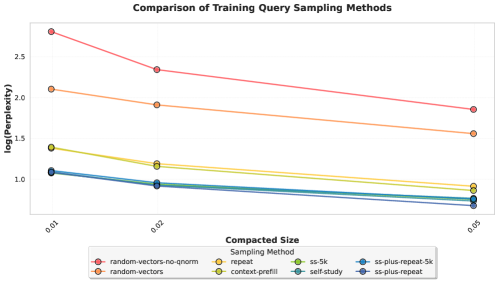<details> <summary>x5.png Details</summary>  ### Visual Description ## Line Chart: Comparison of Training Query Sampling Methods ### Overview The chart compares the log(perplexity) performance of six query sampling methods across three compacted sizes (0.01, 0.02, 0.05). Log(perplexity) is plotted on the y-axis (0–2.75), with lower values indicating better performance. All methods show decreasing perplexity as compacted size increases, but performance varies significantly between methods. ### Components/Axes - **X-axis**: Compacted Size (0.01, 0.02, 0.05) - **Y-axis**: log(Perplexity) (0–2.75, increments of 0.5) - **Legend**: Located at bottom-right, with six color-coded lines: - Red: random-vectors-no-gnorm - Orange: random-vectors - Yellow: repeat - Green: ss-5k - Teal: self-study - Blue: ss-plus-repeat-5k ### Detailed Analysis 1. **random-vectors-no-gnorm (Red)** - Starts at ~2.75 log(perplexity) at 0.01 compacted size. - Decreases linearly to ~1.8 at 0.05. - Highest perplexity across all sizes. 2. **random-vectors (Orange)** - Begins at ~2.1 log(perplexity) at 0.01. - Declines to ~1.5 at 0.05. - Second-highest perplexity. 3. **repeat (Yellow)** - Starts at ~1.3 log(perplexity) at 0.01. - Drops to ~0.9 at 0.05. - Moderate performance. 4. **ss-5k (Green)** - Begins at ~1.2 log(perplexity) at 0.01. - Reduces to ~0.8 at 0.05. - Slightly better than "repeat." 5. **self-study (Teal)** - Starts at ~0.9 log(perplexity) at 0.01. - Decreases to ~0.7 at 0.05. - Near-optimal performance. 6. **ss-plus-repeat-5k (Blue)** - Begins at ~0.8 log(perplexity) at 0.01. - Ends at ~0.6 at 0.05. - **Lowest perplexity**, indicating best performance. ### Key Observations - **Performance Gradient**: All methods improve (lower perplexity) as compacted size increases, but the rate of improvement varies. - **Dominant Outperformer**: "ss-plus-repeat-5k" (blue) consistently outperforms others by ~0.2–0.3 log(perplexity) units. - **Worst Performer**: "random-vectors-no-gnorm" (red) has the highest perplexity, suggesting it is the least effective method. - **Trend Consistency**: All lines slope downward, confirming that larger compacted sizes reduce perplexity. ### Interpretation The chart demonstrates that query sampling methods significantly impact training efficiency, as measured by perplexity. The "ss-plus-repeat-5k" method achieves the lowest perplexity, suggesting it balances compacted size and model performance optimally. Conversely, "random-vectors-no-gnorm" underperforms, likely due to the absence of gnorm regularization. The downward trend across all methods implies that compacted size is a critical factor in reducing perplexity, but method choice determines the magnitude of improvement. This analysis could guide optimization strategies for training query systems, prioritizing methods like "ss-plus-repeat-5k" for efficiency. </details> Figure 5: Reference query sampling comparison. We compare eight variants for sampling queries. Self-study-based methods perform best, especially at the greatest compaction ratios, with repeat and context-prefill close behind. Subsampling reference queries preserves performance. 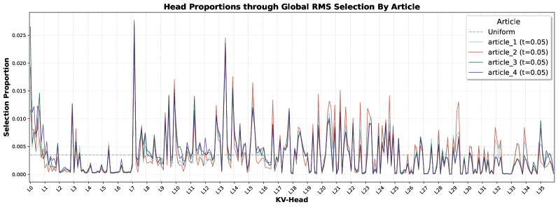## Appendix E Head Budgets <details> <summary>x6.png Details</summary>  ### Visual Description ## Line Graph: Head Proportions through Global RMS Selection By Article ### Overview The image is a line graph visualizing the selection proportions of different articles across 36 KV-Heads (labeled L0 to L35). Four data series (article_1 to article_4) are plotted alongside a dashed "Uniform" baseline. The y-axis represents selection proportion (0.000–0.025), while the x-axis represents KV-Heads. The graph shows significant variability in selection proportions across articles and KV-Heads. ### Components/Axes - **X-Axis (KV-Head)**: Labeled "KV-Head" with discrete markers L0 to L35. - **Y-Axis (Selection Proportion)**: Labeled "Selection Proportion" with a scale from 0.000 to 0.025 in increments of 0.005. - **Legend**: Located in the top-right corner, with four colored lines: - Dashed gray: "Uniform" - Light blue: "article_1 (t=0.05)" - Red: "article_2 (t=0.05)" - Green: "article_3 (t=0.05)" - Purple: "article_4 (t=0.05)" - **Lines**: Four solid-colored lines (light blue, red, green, purple) and one dashed gray line. ### Detailed Analysis 1. **Uniform Baseline**: The dashed gray line remains flat at approximately 0.005 across all KV-Heads, serving as a reference point. 2. **Article_1 (Light Blue)**: - Peaks at L7 (~0.020), L14 (~0.018), and L25 (~0.015). - Troughs near L20 (~0.003) and L30 (~0.002). 3. **Article_2 (Red)**: - Sharpest peak at L7 (~0.025), the highest value in the graph. - Secondary peaks at L14 (~0.022) and L25 (~0.018). - Troughs near L20 (~0.004) and L30 (~0.003). 4. **Article_3 (Green)**: - Peaks at L10 (~0.015), L20 (~0.012), and L30 (~0.010). - Troughs near L5 (~0.002) and L25 (~0.003). 5. **Article_4 (Purple)**: - Peaks at L7 (~0.022), L14 (~0.019), and L25 (~0.016). - Troughs near L5 (~0.001) and L30 (~0.002). ### Key Observations - **Highest Selection Proportion**: Article_2 at L7 (~0.025) exceeds all other values. - **Uniform Baseline**: All articles fluctuate above and below the 0.005 baseline, indicating non-uniform selection. - **Correlated Peaks**: Articles 1, 2, and 4 share prominent peaks at L7, L14, and L25, suggesting shared KV-Head importance. - **Divergent Patterns**: Article_3 exhibits distinct peaks at L10, L20, and L30, differing from other articles. - **Troughs**: All articles show minima near L20 and L30, with Article_4 having the lowest troughs (~0.001–0.002). ### Interpretation The graph demonstrates that selection proportions vary significantly across KV-Heads and articles. The Uniform baseline (0.005) acts as a reference, showing that most articles exceed this value at specific KV-Heads. The shared peaks at L7, L14, and L25 suggest these KV-Heads are critical for multiple articles, while Article_3’s unique pattern highlights distinct selection dynamics. The extreme peak at L7 (article_2) indicates a disproportionately high selection rate at this KV-Head, potentially signaling an outlier or focal point in the selection process. The troughs near L20 and L30 may represent less influential KV-Heads or transitional regions in the selection mechanism. Overall, the data underscores the non-uniform and article-specific nature of KV-Head selection in the Global RMS framework. 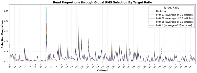</details> <details> <summary>x7.png Details</summary>  ### Visual Description ## Line Graph: Head Proportions through Global RMS Selection By Target Ratio ### Overview The graph illustrates the relationship between KV-Head layers (L0–L35) and selection proportions under varying target ratios (t=0.01, 0.02, 0.05, 0.1) compared to a uniform baseline. Four lines represent different target ratios, with peaks indicating localized increases in selection proportion. ### Components/Axes - **X-Axis (KV-Head)**: Labeled "KV-Head" with discrete markers L0 to L35 (likely representing layers or levels). - **Y-Axis (Selection Proportion)**: Ranges from 0.00 to 0.05 in increments of 0.01. - **Legend**: Positioned in the top-right corner, mapping colors to target ratios: - Dashed gray: Uniform (baseline) - Light blue: t=0.01 (average of 10 articles) - Red: t=0.02 (average of 10 articles) - Green: t=0.05 (average of 10 articles) - Purple: t=0.1 (average of 10 articles) ### Detailed Analysis - **Uniform Baseline (Dashed Gray)**: Remains flat near 0.005 across all L levels, serving as a reference. - **t=0.01 (Light Blue)**: Peaks at L7 (~0.045), with minor fluctuations. Selection proportion drops sharply after L7. - **t=0.02 (Red)**: Peaks at L14 (~0.048), with a secondary peak at L21 (~0.042). Higher magnitude than t=0.01. - **t=0.05 (Green)**: Peaks at L21 (~0.045), with a secondary peak at L28 (~0.04). Broader spread than t=0.02. - **t=0.1 (Purple)**: Peaks at L28 (~0.038), with a secondary peak at L35 (~0.032). Lower magnitude than t=0.05 but wider distribution. ### Key Observations 1. **Peak Correlation**: Higher target ratios (t=0.05, 0.1) exhibit peaks at later L levels (L21, L28, L35) compared to lower ratios (t=0.01, 0.02). 2. **Magnitude Trends**: Peaks for t=0.02 and t=0.05 are the highest (~0.048), while t=0.1 has the lowest peak (~0.038). 3. **Secondary Peaks**: All lines show secondary peaks at later L levels, suggesting sustained selection activity. 4. **Baseline Stability**: The uniform line remains consistently flat, indicating no selection bias without target ratios. ### Interpretation The data suggests that increasing the target ratio correlates with selection proportion peaking at higher KV-Head layers. This implies a hierarchical selection mechanism where larger target ratios engage deeper layers. The uniform baseline confirms that selection proportions are not inherently biased toward specific layers. The secondary peaks may indicate iterative refinement or cascading selection effects. Notably, t=0.1’s lower peak magnitude despite its higher ratio suggests diminishing returns at extreme target values. The sharp drops post-peak could reflect saturation or threshold-based selection criteria. </details> Figure 6: Head proportions induced by global highest-attention selection. We plot the fraction of total selected keys attributed to each of the $288$ KV heads ( $36$ layers, $8$ heads per layer) in Qwen3-4B. Top: proportions across $10$ QuALITY articles at a fixed global compaction ratio of $0.05$ . Bottom: average proportions across multiple global compaction ratios. The low variance across articles and target ratios indicates stable head importance patterns. This appendix provides additional evidence motivating nonuniform KV compaction and visualizes the per-head budgets learned by our method. #### Global key selection induces stable head proportions. KVzip (Kim et al., 2025a) selects keys based on highest attention scores globally across all KV heads, without enforcing per-head quotas. Under a fixed global top- $k$ budget, this induces an implicit allocation in which different heads retain different fractions of the total KV capacity. Figure 6 shows the implicit head proportions induced by global highest-attention selection in Qwen3-4B, supporting the use of a fixed, precomputed nonuniform schedule. #### Head sensitivity curves. Following Section 3.4, we directly measure head sensitivity by varying the compaction ratio of individual heads while holding all other heads fixed. Figure 2 in the main paper shows representative sensitivity curves for Qwen3-4B. To demonstrate that this behavior generalizes across model families, Figure 7 shows analogous head sensitivity curves for Llama-3.1-8B-Instruct. In both models, we observe substantial differences across heads: some heads are largely insensitive to KV capacity, while others benefit significantly from retaining additional keys. 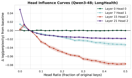<details> <summary>x8.png Details</summary>  ### Visual Description ## Line Graph: Head Influence Curves (Qwen3-4B; LongHealth) ### Overview The graph illustrates the relationship between "Head Ratio" (fraction of original keys) and "Δ log(perplexity) from baseline" for four specific attention heads in the Qwen3-4B model. Four lines represent different layers and heads, showing how reducing the number of keys affects model performance. ### Components/Axes - **X-axis**: Head Ratio (fraction of original keys), ranging from 0.0 to 0.5 in increments of 0.05. - **Y-axis**: Δ log(perplexity) from baseline, ranging from -0.08 to 0.04 in increments of 0.02. - **Legend**: Located in the top-right corner, mapping colors to layers/heads: - Green: Layer 0 Head 0 - Light Blue: Layer 7 Head 1 - Red: Layer 15 Head 2 - Purple: Layer 21 Head 2 ### Detailed Analysis 1. **Layer 0 Head 0 (Green)**: - Remains nearly flat at Δ log(perplexity) ≈ 0.00 across all Head Ratios. - No significant deviation from baseline. 2. **Layer 7 Head 1 (Light Blue)**: - Starts slightly above baseline (Δ ≈ 0.01 at Head Ratio 0.0). - Gradually declines to Δ ≈ -0.02 by Head Ratio 0.5. - Slope: Approximately linear decrease. 3. **Layer 15 Head 2 (Red)**: - Begins at baseline (Δ ≈ 0.00 at Head Ratio 0.0). - Sharp drop to Δ ≈ -0.04 at Head Ratio 0.1. - Continues declining to Δ ≈ -0.08 by Head Ratio 0.5. - Slope: Steeper than Layer 7 Head 1. 4. **Layer 21 Head 2 (Purple)**: - Starts at Δ ≈ 0.04 at Head Ratio 0.0. - Rapid decline to Δ ≈ -0.02 at Head Ratio 0.1. - Stabilizes near Δ ≈ -0.02 for Head Ratios ≥ 0.2. - Slope: Steepest initial drop, then plateau. ### Key Observations - **Layer 0 Head 0** shows no sensitivity to key reduction, suggesting minimal influence on perplexity. - **Layer 21 Head 2** exhibits the most dramatic initial performance drop, indicating critical reliance on full key sets. - **Layer 15 Head 2** demonstrates the largest overall decline, suggesting higher vulnerability to key reduction. - All lines except Layer 0 Head 0 show negative Δ log(perplexity), implying reduced model performance with fewer keys. ### Interpretation The data suggests that higher layers (e.g., Layer 21) and specific heads (e.g., Head 2) are more sensitive to reductions in attention key counts. The sharp initial drop in Layer 21 Head 2 implies these components may rely heavily on full key interactions for optimal performance. The stability of Layer 0 Head 0 indicates it may operate independently of key quantity, possibly handling less critical tasks. These trends highlight architectural trade-offs in attention mechanisms, where certain heads/layers are more critical to model efficacy than others. 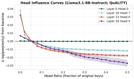</details> <details> <summary>x9.png Details</summary>  ### Visual Description ## Line Chart: Head Influence Curves (Llama3.1-8B-Instruct; QUALITY) ### Overview The chart visualizes the impact of removing attention heads in different layers of the Llama3.1-8B-Instruct model on quality metrics (measured via perplexity). It shows how reducing the number of active heads (head ratio) affects model performance relative to a baseline. ### Components/Axes - **X-axis**: Head Ratio (fraction of original keys) - Scale: 0.0 to 0.5 in increments of 0.1 - Label: "Head Ratio (fraction of original keys)" - **Y-axis**: Δ log(perplexity) from baseline - Scale: -0.03 to 0.04 in increments of 0.01 - Label: "Δ log(perplexity) from baseline" - **Legend**: - **Layer 0 Head 0** (green line) - **Layer 10 Head 7** (light blue line) - **Layer 13 Head 0** (red line) - **Layer 16 Head 5** (purple line) - Legend positioned in the top-right corner. ### Detailed Analysis 1. **Layer 0 Head 0 (Green Line)**: - Remains flat at **0.00** across all head ratios. - Confidence interval (shaded area) is minimal, indicating low variability. 2. **Layer 10 Head 7 (Light Blue Line)**: - Starts at **0.04** (head ratio = 0.0) and decreases linearly to **-0.01** at head ratio = 0.5. - Confidence interval widens slightly but remains narrow. 3. **Layer 13 Head 0 (Red Line)**: - Sharp initial drop from **0.03** (head ratio = 0.0) to **-0.01** (head ratio = 0.1), then stabilizes. - Confidence interval is broader than Layer 0 but narrower than Layer 16. 4. **Layer 16 Head 5 (Purple Line)**: - Gradual decline from **0.01** (head ratio = 0.0) to **-0.03** (head ratio = 0.5). - Confidence interval widens significantly, showing higher uncertainty. ### Key Observations - **Layer 0 Head 0** is the only head with no measurable impact on perplexity, suggesting it may be redundant or optimized during training. - **Layer 13 Head 0** exhibits the most dramatic initial performance drop, indicating critical importance in early stages of head removal. - **Layer 16 Head 5** shows the most consistent negative trend, implying a strong dependency on this head for maintaining quality. - Confidence intervals suggest **Layer 0** has the most reliable measurements, while **Layer 16** has the highest variability. ### Interpretation The data demonstrates that removing attention heads generally degrades model quality (higher perplexity), with effects varying by layer and head. Layer 0 Head 0’s stability suggests it may not contribute meaningfully to performance, while Layer 13 Head 0’s sharp decline highlights its critical role. The widening confidence intervals for Layer 16 Head 5 imply greater uncertainty in its influence, possibly due to architectural complexity or training dynamics. These results underscore the importance of head-specific analysis in model optimization and pruning strategies. </details> Figure 7: More Head sensitivity curves. Analogous to Figure 2, showing loss change as a function of per-head compaction ratio for four selected heads. Left: Qwen3-4B with LongHealth exhibits similar patterns to Figure 2. Right: Llama-3.1-8B-Instruct also shows head-dependent sensitivity patterns: some heads are largely insensitive to KV capacity, while others benefit substantially from retaining more keys. #### Optimized head budgets. Algorithm 4 Nonuniform KV Allocation via Greedy Swaps 0: Heads $h=1,\dots,H$ ; step size $η>0$ (share units); per-head sensitivity curves $J_h(ρ)$ mapping compaction ratio $ρ∈[0,1]$ to loss; reference overall compaction ratio $r_0$ (we use $r_0=0.05$ ). 0: Shares $\{p_h\}$ with $∑_hp_h=1$ and $p_h≥ 0$ . 1: Initialize. $p_h←\frac{1}{H}$ for all $h$ . 2: repeat 3: Map shares to ratios. $ρ_h← p_h· H· r_0$ for all $h$ . 4: Compute marginals. For each head $h$ , $$ g_h^+←\begin{cases}J_h(ρ_h)-J_h(ρ_h+η^\prime),&if ρ_h+η^\prime≤ 1,\\ -∞,&otherwise,\end{cases} g_h^-←\begin{cases}J_h(ρ_h-η^\prime)-J_h(ρ_h),&if ρ_h≥η^\prime,\\ +∞,&otherwise,\end{cases} $$ where $η^\prime=η· H· r_0$ is the step size in ratio space. 5: Select best swap. $b^⋆←\arg\max_h g_h^+$ , $a^⋆←\arg\min_h g_h^-$ with $a^⋆≠ b^⋆$ . 6: if $g_b^⋆^+>g_a^⋆^-$ then 7: $p_a^⋆← p_a^⋆-η; p_b^⋆← p_b^⋆+η.$ 8: else 9: break {No improving swap remains.} 10: end if 11: until termination 12: return $\{p_h\}$ . Using these sensitivity curves, we apply the budget-allocation procedure described in Section 3.4 and Algorithm 4 to derive model-specific nonuniform head budgets. Figure 8 compares the resulting optimized head proportions to the average head proportions induced by global highest-attention key selection. 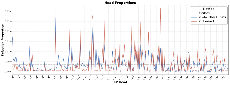<details> <summary>x10.png Details</summary>  ### Visual Description ## Line Graph: Head Proportions ### Overview The graph compares three methods (Uniform, Global RMS t=0.05, Optimized) across 36 KV-Heads (L0–L35) in terms of "Selection Proportion." The y-axis ranges from 0.000 to 0.030, with the Uniform method represented by a dashed gray line, Global RMS by a solid blue line, and Optimized by a solid red line. ### Components/Axes - **X-Axis (KV-Head)**: Labeled from L0 to L35, representing discrete heads. - **Y-Axis (Selection Proportion)**: Scaled from 0.000 to 0.030 in increments of 0.005. - **Legend**: Located in the top-right corner, mapping colors to methods: - Dashed gray: Uniform - Solid blue: Global RMS t=0.05 - Solid red: Optimized ### Detailed Analysis 1. **Uniform (Dashed Gray)**: - Remains consistently low (0.000–0.005) across all KV-Heads. - Minor fluctuations observed at L1, L3, L5, and L35 (~0.003–0.004). 2. **Global RMS t=0.05 (Solid Blue)**: - Peaks at L7 (~0.026), L14 (~0.024), L21 (~0.022), L28 (~0.020), and L35 (~0.018). - Intermediate values (~0.005–0.015) at other heads. - Smoother transitions between peaks compared to Optimized. 3. **Optimized (Solid Red)**: - Sharp, tall peaks at L7 (~0.028), L14 (~0.026), L21 (~0.024), L28 (~0.022), and L35 (~0.020). - Secondary peaks at L2 (~0.012), L9 (~0.015), L16 (~0.018), L23 (~0.016), and L31 (~0.014). - Remains near 0.000–0.005 at most other heads. ### Key Observations - **Peak Correlation**: All methods show elevated proportions at L7, L14, L21, L28, and L35, with Optimized peaking highest. - **Optimized Dominance**: The Optimized method consistently allocates 1.5–2× higher proportions than Global RMS and 3–5× higher than Uniform at peak heads. - **Uniform Stability**: The Uniform method shows minimal variation, suggesting a baseline or control condition. ### Interpretation The data suggests the **Optimized method** prioritizes specific KV-Heads (L7, L14, L21, L28, L35) significantly more than the other methods, potentially indicating targeted efficiency or resource allocation. The Global RMS method exhibits moderate selectivity, while the Uniform method acts as a near-zero baseline. The recurring peaks in Optimized and Global RMS at specific heads imply these components are critical to the system’s performance, warranting further investigation into their functional roles. The absence of peaks in Uniform reinforces its role as a control or reference. </details> Figure 8: Optimized head budgets. We compare the head proportions learned by our nonuniform allocation algorithm to those induced by global highest-attention key selection. The optimized schedule has similar structure as the global highest attention scores schedule. The optimized schedule tends to assign more budget to later layers and less to earlier layers, contrary to PyramidKV (Cai et al., 2025). ## Appendix F Further Results ### F.1 Mean vs. RMS vs. Max Aggregation Several prior methods—including H2O, SnapKV, PyramidKV, KVzip, and our AM-HighestAttnKeys —select a subset of keys based on attention scores under a collection of query vectors. Concretely, for each key $K_j$ and reference query $\bm{q}_i$ , we compute the attention weight $$ a_i,j=(\bm{q}_i\bm{K}^⊤)_j. $$ To rank keys globally, these per-query attention weights must be aggregated across queries into a single importance score per key, after which the top- $t$ keys are retained. We consider three aggregation functions: $$ s_j^mean=\frac{1}{n}∑_i=1^na_i,j, s_j^rms=√{\frac{1}{n}∑_i=1^na_i,j^2}, s_j^max=\max_ia_i,j. $$ Figure 9 compares downstream performance across these choices for four baseline methods as well as our Highest Attention Keys approach. There is no choice that is consistently best across methods, though RMS offers a good balance and we adopt it in our method. 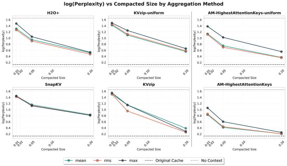<details> <summary>x11.png Details</summary>  ### Visual Description ## Line Graphs: log(Perplexity) vs Compacted Size by Aggregation Method ### Overview The image contains six line graphs comparing the logarithmic perplexity (log(Perplexity)) of different aggregation methods (H2O+, KVzip-uniform, AM-HighestAttentionKeys-uniform, SnapKV, KVzip, AM-HighestAttentionKeys) against compacted size. Each graph includes three data series: **mean** (teal), **rms** (orange), and **max** (dark blue), alongside two reference lines: **Original Cache** (dashed) and **No Context** (dotted). The x-axis represents compacted size (0.01 to 0.20), and the y-axis represents log(Perplexity) (0.2 to 1.6). ### Components/Axes - **X-axis (Compacted Size)**: Logarithmic scale from 0.01 to 0.20. - **Y-axis (log(Perplexity))**: Logarithmic scale from 0.2 to 1.6. - **Legends**: - **Mean** (teal circle) - **RMS** (orange circle) - **Max** (dark blue circle) - **Original Cache** (dashed line) - **No Context** (dotted line) - **Graph Titles**: Each subplot is labeled with the aggregation method (e.g., "H2O+", "KVzip-uniform"). ### Detailed Analysis #### H2O+ - **Mean**: Starts at ~1.3 (0.01) and decreases to ~0.4 (0.20). - **RMS**: Slightly lower than mean, starting at ~1.25 (0.01) and ending at ~0.35 (0.20). - **Max**: Peaks at ~1.45 (0.01) and drops to ~0.5 (0.20). - **Original Cache**: Consistently above all data series (~1.5–1.6). - **No Context**: Lowest line (~0.2–0.3). #### KVzip-uniform - **Mean**: Starts at ~1.4 (0.01) and decreases to ~0.5 (0.20). - **RMS**: Slightly lower than mean, starting at ~1.35 (0.01) and ending at ~0.4 (0.20). - **Max**: Peaks at ~1.5 (0.01) and drops to ~0.6 (0.20). - **Original Cache**: ~1.5–1.6. - **No Context**: ~0.2–0.3. #### AM-HighestAttentionKeys-uniform - **Mean**: Starts at ~1.3 (0.01) and decreases to ~0.4 (0.20). - **RMS**: Slightly lower than mean, starting at ~1.25 (0.01) and ending at ~0.35 (0.20). - **Max**: Peaks at ~1.4 (0.01) and drops to ~0.5 (0.20). - **Original Cache**: ~1.5–1.6. - **No Context**: ~0.2–0.3. #### SnapKV - **Mean**: Starts at ~1.4 (0.01) and decreases to ~0.8 (0.20). - **RMS**: Slightly lower than mean, starting at ~1.35 (0.01) and ending at ~0.7 (0.20). - **Max**: Peaks at ~1.5 (0.01) and drops to ~0.9 (0.20). - **Original Cache**: ~1.5–1.6. - **No Context**: ~0.2–0.3. #### KVzip - **Mean**: Starts at ~1.4 (0.01) and decreases to ~0.3 (0.20). - **RMS**: Slightly lower than mean, starting at ~1.35 (0.01) and ending at ~0.25 (0.20). - **Max**: Peaks at ~1.5 (0.01) and drops to ~0.4 (0.20). - **Original Cache**: ~1.5–1.6. - **No Context**: ~0.2–0.3. #### AM-HighestAttentionKeys - **Mean**: Starts at ~1.3 (0.01) and decreases to ~0.2 (0.20). - **RMS**: Slightly lower than mean, starting at ~1.25 (0.01) and ending at ~0.15 (0.20). - **Max**: Peaks at ~1.4 (0.01) and drops to ~0.3 (0.20). - **Original Cache**: ~1.5–1.6. - **No Context**: ~0.2–0.3. ### Key Observations 1. **Trend**: All data series show a **decreasing trend** in log(Perplexity) as compacted size increases, indicating improved performance with larger compacted sizes. 2. **Original Cache**: Consistently the highest line across all methods, suggesting it is the least effective at reducing perplexity. 3. **No Context**: The lowest line in all graphs, indicating it performs the worst. 4. **Method-Specific Performance**: - **AM-HighestAttentionKeys** and **KVzip** show the steepest declines, suggesting they are more efficient at reducing perplexity. - **SnapKV** and **H2O+** have moderate declines, while **KVzip-uniform** and **AM-HighestAttentionKeys-uniform** show similar trends to their non-uniform counterparts. 5. **Outliers**: The **Original Cache** line is consistently above all data series, highlighting its inefficiency compared to other methods. ### Interpretation The data demonstrates that **aggregation methods** significantly impact perplexity reduction as models are compacted. Lower log(Perplexity) values (closer to the "No Context" line) indicate better performance. The **Original Cache** line’s consistent high values suggest it is a suboptimal baseline, while methods like **AM-HighestAttentionKeys** and **KVzip** outperform others, likely due to their attention-based or compression-focused strategies. The **No Context** line underscores the importance of contextual information in maintaining low perplexity. These trends align with the hypothesis that advanced aggregation techniques (e.g., attention mechanisms) are more effective at preserving model performance during compression. </details> Figure 9: Effect of aggregation function on key selection. We plot accuracy versus compaction ratio for four baseline methods and our Highest Attention Keys method on a subset of $20$ QuALITY articles using Qwen3-4B. All methods select the top- $t$ keys based on aggregated attention scores over a shared set of reference queries. ### F.2 Reconstruction vs. Downstream Accuracy In addition to QA accuracy, we also compute loss (log-perplexity) on the original-cache generations: we evaluate the negative log-likelihood of responses sampled from the full cache, but conditioned on the compacted cache. This metric measures how well a compacted cache preserves the model’s token-level behavior, differing from the forward KL divergence only by a constant additive term. Figure 1 (left) replicates our main trade-off plot using this loss metric, and Figure 10 (right) compares downstream multiple-choice accuracy directly against log-perplexity across methods and compaction ratios. Across attention-matching methods and token-selection baselines, we observe that points roughly interpolate between the no-context results (high loss, low accuracy) and the full-context results (low loss, high accuracy). As expected, improvements in reconstruction tend to translate into improvements in QA accuracy. Two notable deviations from this trend are Cartridges and summarization. Cartridges tends to achieve slightly lower reconstruction loss than methods with similar downstream accuracy, consistent with its objective: it performs end-to-end latent-cache optimization using a distillation-style loss that targets the original model’s behavior, directly optimizing token-level fidelity. In contrast, summarization often yields higher reconstruction loss than methods with similar accuracy: it discards substantial token-level detail but can preserve (or even emphasize) the subset of information most useful for answering comprehension questions. In other words, summarization can be a good task heuristic despite being a poor reconstruction mechanism. Overall, these results support two conclusions: (i) reconstruction loss is a useful proxy for comparing compaction methods within families that aim to preserve attention behavior, and (ii) it should not be treated as a universal predictor of downstream performance when methods fundamentally change the objective. We further note that self-log-perplexity in long-context evaluations can be skewed on many language models due to entropy blowup as generations grow longer (Braverman et al., 2020; Cao et al., 2025). The perplexity numbers reported here are for Qwen3-4B on QuALITY (contexts $<10$ k tokens), where we did not observe such entropy blowup, though we did observe this at longer context lengths. 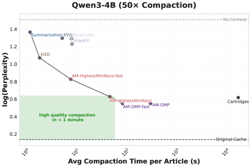<details> <summary>x12.png Details</summary>  ### Visual Description ## Scatter Plot: Qwen3-4B (50x Compaction) ### Overview This scatter plot compares the relationship between **compaction time per article** (x-axis) and **perplexity** (y-axis) for various Qwen3-4B model compression techniques. It includes labeled data points, a shaded "high quality" region, and reference lines for context. --- ### Components/Axes - **Title**: "Qwen3-4B (50x Compaction)" - **X-axis**: - Label: "Avg Compaction Time per Article (s)" - Scale: Logarithmic (10⁰ to 10⁴) - Tick marks: 10⁰, 10¹, 10², 10³, 10⁴ - **Y-axis**: - Label: "log(Perplexity)" - Scale: Linear (0.2 to 1.4) - Tick marks: 0.2, 0.4, 0.6, 0.8, 1.0, 1.2, 1.4 - **Legend**: - Located at the top-left of the plot. - Colors: - Red: "AM-HighestAttnKeys-fast" - Purple: "AM-OMP" - Gray: "No-Context" (dashed line) - Black: "Original-Cache" (dashed line) - **Shaded Region**: - Green rectangle labeled "high quality compaction in < 1 minute" - Bounds: X = 10⁰–10² s, Y = 0.4–0.6 --- ### Detailed Analysis 1. **Data Points**: - **H2O**: (10⁰ s, 1.1 perplexity) - **Summarization KVzl**: (10⁰.⁵ s, 1.3 perplexity) - **SnapKV**: (10¹ s, 1.25 perplexity) - **AM-HighestAttnKeys**: (10¹.⁵ s, 0.65 perplexity) - **AM-HighestAttnKeys-fast**: (10¹.⁵ s, 0.8 perplexity) - **AM-OMP**: (10² s, 0.55 perplexity) - **AM-OMP-fast**: (10² s, 0.6 perplexity) - **Cartridges**: (10⁴ s, 0.6 perplexity) 2. **Trends**: - A diagonal trendline connects H2O → Summarization KVzl → SnapKV → AM-HighestAttnKeys → AM-OMP, showing **increasing compaction time** with **decreasing perplexity**. - AM-OMP-fast and AM-HighestAttnKeys-fast cluster in the "high quality" region (green shaded area). - Cartridges deviates to the far right (10⁴ s) with moderate perplexity. 3. **Reference Lines**: - "No-Context" (dashed horizontal line at Y = 1.4). - "Original-Cache" (dashed horizontal line at Y = 0.2). --- ### Key Observations - **Efficiency Tradeoff**: Most methods cluster in the "high quality" region, balancing speed and low perplexity. - **Outliers**: - **Cartridges** requires 10⁴ s (10,000x slower than H2O) but achieves the same perplexity as AM-OMP. - **AM-HighestAttnKeys-fast** and **AM-OMP-fast** achieve near-optimal perplexity (<0.6) within the <1-minute compaction window. - **Baselines**: - "No-Context" represents the worst-case perplexity (1.4). - "Original-Cache" represents the best-case perplexity (0.2). --- ### Interpretation The plot demonstrates that **AM-OMP** and **AM-HighestAttnKeys** variants offer the best compromise between speed and quality, achieving low perplexity (<0.6) within the "high quality" region (<1 minute). **Cartridges** is an outlier, suggesting either inefficiency or specialized use cases. The diagonal trendline implies a general inverse relationship between compaction time and perplexity, though exceptions exist. The "No-Context" and "Original-Cache" lines frame the performance boundaries, highlighting that most methods outperform baseline caching strategies. **Critical Insight**: Methods labeled with "-fast" suffixes (e.g., AM-HighestAttnKeys-fast) prioritize speed without sacrificing quality, making them ideal for real-time applications. 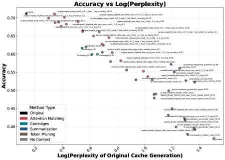</details> <details> <summary>x13.png Details</summary>  ### Visual Description ## Scatter Plot: Accuracy vs Log(Perplexity) ### Overview The image is a scatter plot comparing **Accuracy** (y-axis) against **Log(Perplexity of Original Cache Generation)** (x-axis). Data points are color-coded by method type, with labels indicating specific configurations or parameters. The plot visualizes trade-offs between model performance (accuracy) and computational complexity (perplexity). --- ### Components/Axes - **X-axis**: Log(Perplexity of Original Cache Generation) - Range: 0.2 to 1.4 - Labels: Numerical values (0.2, 0.4, 0.6, 0.8, 1.0, 1.2, 1.4) - **Y-axis**: Accuracy - Range: 0.40 to 0.70 - Labels: Numerical values (0.40, 0.45, 0.50, 0.55, 0.60, 0.65, 0.70) - **Legend**: Located in the bottom-left corner, mapping colors to method types: - **Black**: Original - **Red**: Attention Matching - **Teal**: Cartridges - **Blue**: Summarization - **Brown**: Token Pruning - **Gray**: No Context --- ### Detailed Analysis #### Data Points and Labels - **Original (Black)**: - Highest accuracy (~0.70) and lowest perplexity (~0.2). - Label: "original" - **Attention Matching (Red)**: - Accuracy ~0.65–0.70, perplexity ~0.3–0.5. - Labels: "attention_matching_highest_attn_keys_mean_nobeta_direct_10.00", "attention_matching_highest_attn_keys_mean_nobeta_direct_10.01" - **Cartridges (Teal)**: - Accuracy ~0.55–0.60, perplexity ~0.6–0.8. - Labels: "cartridges_10.00", "cartridges_10.01" - **Summarization (Blue)**: - Accuracy ~0.50–0.55, perplexity ~0.8–1.0. - Labels: "summarization_highest_attn_keys_mean_nobeta_direct_10.00", "summarization_highest_attn_keys_mean_nobeta_direct_10.01" - **Token Pruning (Brown)**: - Accuracy ~0.45–0.50, perplexity ~1.0–1.2. - Labels: "token_pruning_highest_attn_keys_mean_nobeta_direct_10.00", "token_pruning_highest_attn_keys_mean_nobeta_direct_10.01" - **No Context (Gray)**: - Lowest accuracy (~0.40–0.45), highest perplexity (~1.2–1.4). - Labels: "no_context_highest_attn_keys_mean_nobeta_direct_10.00", "no_context_highest_attn_keys_mean_nobeta_direct_10.01" #### Trends - **Inverse Relationship**: Higher perplexity (x-axis) generally correlates with lower accuracy (y-axis). - **Method-Specific Performance**: - **Original** and **Attention Matching** dominate the top-left (high accuracy, low perplexity). - **Cartridges** and **Summarization** cluster in the middle, showing moderate trade-offs. - **Token Pruning** and **No Context** occupy the bottom-right (low accuracy, high perplexity). --- ### Key Observations 1. **Original Method**: Optimal performance (highest accuracy, lowest perplexity). 2. **Attention Matching**: Slightly lower accuracy than Original but still high, with slightly higher perplexity. 3. **Cartridges**: Moderate accuracy and perplexity, suggesting a balance between complexity and performance. 4. **Summarization**: Lower accuracy than Cartridges despite similar perplexity, indicating potential inefficiencies. 5. **Token Pruning/No Context**: Poor performance, with high perplexity and low accuracy. --- ### Interpretation The plot highlights a clear trade-off between **model complexity (perplexity)** and **performance (accuracy)**. The **Original** and **Attention Matching** methods outperform others by maintaining high accuracy with minimal perplexity, suggesting they are more efficient or well-optimized. In contrast, **Token Pruning** and **No Context** methods degrade performance significantly, likely due to excessive simplification or lack of contextual information. The **Cartridges** and **Summarization** methods occupy a middle ground, indicating that while they reduce perplexity compared to Token Pruning/No Context, their accuracy drops compared to Original/Attention Matching. This suggests that methods like Cartridges may prioritize computational efficiency over accuracy, while Summarization might introduce bottlenecks. The **No Context** method’s extreme position (lowest accuracy, highest perplexity) underscores the importance of contextual information in model performance. **Notable Anomalies**: - Some labels (e.g., "context_profile_highest_attn_keys_mean_nobeta_direct_10.00") imply specific configurations, but their exact impact on performance is not quantified in the plot. - The "original" method’s dominance suggests it may serve as a baseline for comparison. This analysis emphasizes the need to balance model complexity with practical performance requirements, depending on the use case. </details> Figure 10: Reconstruction loss vs. downstream accuracy. Left: Loss-based analogue of Figure 1, instead reporting log-perplexity on original-cache generations. Right: Downstream multiple-choice accuracy plotted against this loss across various methods and compaction ratios. ### F.3 Extension: Online Compaction For long-horizon reasoning, we may want to compact mid-trajectory so the model can continue decoding after producing thousands of intermediate tokens. | Phys Len | Eff Len | AIME (/30) | Notes | | --- | --- | --- | --- | | 2048 | 2048 | 1.25 | | | 4096 | 4096 | 7.75 | | | 8192 | 8192 | 13 | | | With online compaction | | | | | 2048 | 4096 | 8 | $≤$ 2 compactions | | 2048 | 8192 | 13 | $≤$ 6 compactions | Table 7: AIME performance (pass@1, averaged over 4 runs) with and without mid-trajectory compaction. Effective sequence length is the total number of decoded tokens, while physical sequence length is the maximum physical size of the KV cache. Each compaction reduces the size of the entire KV cache (including previously compacted portions) by $50\$ , so $≤$ 2 and $≤$ 6 compactions correspond to approximately $2×$ and $4×$ more decoded tokens, respectively. For implementation simplicity, we do not enable non-uniform compaction or on-policy queries. We use AM-HighestAttnKeys-Fast. We believe more tuned methods (e.g. with higher compaction ratios, compacting only the most recently generated tokens, etc.) may improve results. We conduct a proof-of-concept evaluation of online compaction on AIME 2025 with Qwen3-4B. For each problem, we cap the physical sequence length during reasoning to a fixed budget (Phys Len). Whenever the model reaches this budget, we compact the entire context except for the most recent $20$ tokens, and then continue decoding until reaching a target effective decoding length (Eff Len). We compare against standard decoding to the same effective length without any compaction. To control token budgets, when the model reaches the maximum context length we inject \nI need to respond with the answer.\n</think>Final Answer:> (following Muennighoff et al. (2025)) and decode the final answer. Overall, these results suggest that online compaction can effectively decouple reasoning depth from physical context limits. Despite shrinking the KV cache mid-trajectory up to six consecutive times, the model achieves performance comparable to standard decoding at the same effective length, indicating that essential reasoning state is largely preserved. Our study uses a simple uniform compaction scheme and always compacts the entire context, rather than, for example, freezing previously compacted portions or selectively compacting recent tokens. We believe that more careful tuning could enable much greater scaling. We present these results primarily to demonstrate the strong empirical stability of reasoning under repeated mid-trajectory compaction. Finally, extending online compaction to multi-turn settings, such as compacting long tool call outputs, remains an interesting application for future work.