# SRFed: Mitigating Poisoning Attacks in Privacy-Preserving Federated Learning with Heterogeneous Data
**Authors**:
- Yiwen Lu1,2Corresponding Author (School of Mathematics, Nanjing University, Nanjing 210093, China)
- 2E-mail: luyw@smail.nju.edu.cn
Abstract
Federated Learning (FL) enables collaborative model training without exposing clients’ private data, and has been widely adopted in privacy-sensitive scenarios. However, FL faces two critical security threats: curious servers that may launch inference attacks to reconstruct clients’ private data, and compromised clients that can launch poisoning attacks to disrupt model aggregation. Existing solutions mitigate these attacks by combining mainstream privacy-preserving techniques with defensive aggregation strategies. However, they either incur high computation and communication overhead or perform poorly under non-independent and identically distributed (Non-IID) data settings. To tackle these challenges, we propose SRFed, an efficient Byzantine-robust and privacy-preserving FL framework for Non-IID scenarios. First, we design a decentralized efficient functional encryption (DEFE) scheme to support efficient model encryption and non-interactive decryption. DEFE also eliminates third-party reliance and defends against server-side inference attacks. Second, we develop a privacy-preserving defensive model aggregation mechanism based on DEFE. This mechanism filters poisonous models under Non-IID data by layer-wise projection and clustering-based analysis. Theoretical analysis and extensive experiments show that SRFed outperforms state-of-the-art baselines in privacy protection, Byzantine robustness, and efficiency.
I Introduction
Federated learning (FL) has emerged as a promising paradigm for distributed machine learning, which enables multiple clients to collaboratively train a global model without sharing their private data. In a typical FL setup, multiple clients periodically train local models using their private data and upload model updates to a central server, which aggregates these updates to obtain a global model with enhanced performance. Due to its ability to protect data privacy, FL has been widely applied in real-world scenarios, such as intelligent driving [1, 2, 3, 4, 5], medical diagnosis [6, 7, 8, 9], and intelligent recommendation systems [10, 11, 12, 13].
Although FL avoids direct data exposure, it is not immune to privacy and security risks. Existing studies [14, 15, 16] have shown that the curious server may launch inference attacks to reconstruct sensitive data samples of clients from the model updates. This may lead to the leakage of clients’ sensitive information, e.g., medical diagnosis records, which can be exploited by adversaries for launching further malicious activities. Moreover, FL is also vulnerable to poisoning attacks [17, 18, 19]. The adversaries may manipulate some clients to execute malicious local training and upload poisonous model updates to mislead the global model [18, 20, 21]. This attack will damage the performance of the global model and lead to incorrect decisions in downstream tasks such as medical diagnosis and intelligent driving.
To address privacy leakage issues, existing privacy-preserving federated learning (PPFL) methods primarily rely on techniques such as differential privacy (DP) [22, 23, 24, 25, 26], secure multi-party computation (SMC) [27, 28], and homomorphic encryption (HE) [29, 30]. However, DP typically leads to a reduction in global model accuracy, while SMC and HE incur substantial computational and communication overheads in FL. Recently, lightweight functional encryption (FE) schemes [31, 32] have been applied in FL. FE enables the server to aggregate encrypted models and directly obtain the decrypted results via a functional key, which avoids the accuracy loss in DP and the extra communication overhead in HE/SMC. However, existing FE schemes rely on third parties for functional key generation, which introduces potential privacy risks.
To mitigate poisoning attacks, existing Byzantine-robust FL methods [33, 34, 35, 36] typically adopt defensive aggregation strategies, which filter out malicious model updates based on statistical distances or performance-based criteria. However, these strategies rely on the assumption that clients’ data distributions are homogeneous, leading to poor performance in non-independent and identically distributed (Non-IID) data settings. Moreover, they require access to plaintext model updates, which directly contradicts the design goal of PPFL [32]. Recently, privacy-preserving Byzantine-robust FL methods [37, 29] have been proposed to address both privacy and poisoning attacks. However, these methods still suffer from limitations such as accuracy loss, excessive overhead, and limited effectiveness in Non-IID environments, as they merely combine the PPFL with existing defensive aggregation strategies. As a result, there is still a lack of practical solutions that can simultaneously ensure privacy protection and Byzantine robustness in Non-IID data scenarios.
To address the limitations of existing FL solutions, we propose a novel Byzantine-robust privacy-preserving FL method, SRFed. SRFed achieves efficient privacy protection and Byzantine robustness in Non-IID data scenarios through two key designs. First, we propose a new functional encryption scheme, DEFE, to protect clients’ model privacy and resist inference attacks from the server. Compared with existing FE schemes, DEFE eliminates reliance on third parties through distributed key generation and improves decryption efficiency by reconstructing the ciphertext. Second, we develop a privacy-preserving robust aggregation strategy based on secure layer-wise projection and clustering. This strategy resists the poisoning attacks in Non-IID data scenarios. Specifically, this strategy first decomposes client models layer by layer, projects each layer onto the corresponding layer of the global model. Then, it performs clustering analysis on the projection vectors to filter malicious updates and aggregates the remaining benign models. DEFE supports the above secure layer-wise projection computation and enables privacy-preserving model aggregation. Finally, we evaluate SRFed on multiple datasets with varying levels of heterogeneity. Theoretical analysis and experimental results demonstrate that SRFed achieves strong privacy protection, Byzantine robustness, and high efficiency. In summary, the core contributions of this paper are as follows.
- We propose a novel secure and robust FL method, SRFed, which simultaneously guarantees privacy protection and Byzantine robustness in Non-IID data scenarios.
- We design an efficient functional encryption scheme, which not only effectively protects the local model privacy but also enables efficient and secure model aggregation.
- We develop a privacy-preserving robust aggregation strategy, which effectively defends against poisoning attacks in Non-IID scenarios and generates high-quality aggregated models.
- We implement the prototype of SRFed and validate its performance in terms of privacy preservation, Byzantine robustness, and computational efficiency. Experimental results show that SRFed outperforms state-of-the-art baselines in all aspects.
II Related Works
II-A Privacy-Preserving Federated Learning
To safeguard user privacy, current research on privacy-preserving federated learning (PPFL) mainly focuses on protecting gradient information. Existing solutions are primarily built upon four core technologies: Differential Privacy (DP) [22, 23, 24], Secure Multi-Party Computation (SMC) [27, 28], Homomorphic Encryption (HE) [29, 38, 30], and Functional Encryption (FE) [31, 32, 39, 40]. DP achieves data indistinguishability by injecting calibrated noise into raw data, thus ensuring privacy with low computational overhead. Miao et al. [24] proposed a DP-based ESFL framework that adopts adaptive local DP to protect data privacy. However, the injected noise inevitably degrades the model accuracy. To avoid accuracy loss, SMC and HE employ cryptographic primitives to achieve privacy preservation. SMC enables distributed aggregation while keeping local gradients confidential, revealing only the aggregated model update. Zhang et al. [27] introduced LSFL, a secure FL framework that applies secret sharing to split and transmit local parameters to two non-colluding servers for privacy-preserving aggregation. HE allows direct computation on encrypted data and produces decrypted results identical to plaintext computations. This property preserves privacy without sacrificing accuracy. Ma et al. [29] developed ShieldFL, a robust FL framework based on two-trapdoor HE, which encrypts all local gradients and achieves aggregation of encrypted gradients. Despite their strong privacy guarantees, SMC/HE-based FL methods incur substantial computation and communication overhead, posing challenges for large-scale deployment. To address these issues, FE has been introduced into FL. FE avoids noise injection and eliminates the high overhead caused by multi-round interactions or complex homomorphic operations. Chen et al. [31] proposed ESB-FL, an efficient secure FL framework based on non-interactive designated decrypter FE (NDD-FE), which protects local data privacy but relies on a trusted third-party entity. Yu et al. [40] further proposed PrivLDFL, which employs a dynamic decentralized multi-client FE (DDMCFE) scheme to preserve privacy in decentralized settings. However, both FE-based methods require discrete logarithm-based decryption, which is typically a time-consuming operation. To overcome these limitations, we propose a decentralized efficient functional encryption (DEFE) scheme that achieves privacy protection and high computational and communication efficiency.
TABLE I: COMPARISON BETWEEN OUR METHOD WITH PREVIOUS WORK
| Methods | Privacy Protection | Defense Mechanism | Efficient | Non-IID | Fidelity |
| --- | --- | --- | --- | --- | --- |
| ESFL [24] | Local DP | Local DP | ✓ | ✗ | ✗ |
| PBFL [37] | CKKS | Cosine similarity | ✗ | ✗ | ✓ |
| ESB-FL [31] | NDD-FE | ✗ | ✓ | ✗ | ✓ |
| Median [35] | ✗ | Median | ✓ | ✗ | ✓ |
| FoolsGold [33] | ✗ | Cosine similarity | ✓ | ✗ | ✓ |
| ShieldFL [29] | HE | Cosine similarity | ✗ | ✗ | ✓ |
| PrivLDFL [40] | DDMCFE | ✗ | ✓ | ✗ | ✓ |
| Biscotti [41] | DP | Euclidean distance | ✓ | ✗ | ✗ |
| SRFed | DEFE | Layer-wise projection and clustering | ✓ | ✓ | ✓ |
- Notes: The symbol ”✓” indicates that it owns this property; ”✗” indicates that it does not own this property. ”Fidelity” indicates that the method has no accuracy loss when there is no attack. ”Non-IID” indicates that the method is Byzantine-Robust under Non-IID data environments.
II-B Privacy-Preserving Federated Learning Against Malicious Participants
To resist poisoning attacks, several defensive aggregation rules have been proposed in FL. FoolsGold [33], proposed by Fung et al. [33], reweights clients’ contributions by computing the cosine similarity of their historical gradients. Krum [34] selects a single client update that is closest, in terms of Euclidean distance, to the majority of other updates in each iteration. Median [35] mitigates the effect of malicious clients by taking the median value of each model parameter across all clients. However, the above aggregation rules require access to plaintext model updates. This makes them unsuitable for direct application in PPFL. To achieve Byzantine-robust PPFL, Shiyan et al. [41] proposed Biscotti. Biscotti leverages DP to protect local gradients while using the Krum algorithm to mitigate poisoning attacks. Nevertheless, the injected noise in DP reduces the accuracy of the aggregated model. To overcome this limitation, Zhang et al. [27] proposed LSFL. LSFL employs SMC to preserve privacy and uses Median-based aggregation for poisoning defense. However, its dual-server architecture introduces significant communication overhead. In addition, Ma et al. [29] and Miao et al. [37] proposed ShieldFL and PBFL, respectively. Both schemes adopt HE to protect local gradients and cosine similarity to defend against poisoning attacks. However, they suffer from high computational complexity and limited robustness under non-IID data settings. To address these challenges, we propose a novel Byzantine-robust and privacy-preserving federated learning method. Table I compares previous schemes with our method.
III Problem Statement
III-A System Model
The system model of SRFed comprises two roles: the aggregation server and clients.
- Clients: Clients are nodes with limited computing power and heterogeneous data. In real-world scenarios, data heterogeneity typically arises across clients (e.g., intelligent vehicles) due to differences in usage patterns, such as driving habits. Each client is responsible for training its local model based on its own data. To protect data privacy, the models are encrypted and submitted to the server for aggregation.
- Server: The server is a node with strong computing power (e.g., service provider of intelligent vehicles). It collects encrypted local models from clients, conducts model detection, and then aggregates selected models and distributes the aggregated model back to clients for the next training round.
III-B Threat Model
We consider the following threat model:
1) Honest-But-Curious server: The server honestly follows the FL protocol but attempts to infer clients’ private data. Specifically, upon receiving encrypted local models from the clients, the server may launch inference attacks on the encrypted models and exploit intermediate computational results (e.g., layer-wise projections and aggregated outputs) to extract sensitive information of clients.
2) Malicious clients: We consider a FL scenario where a certain proportion of clients are malicious. These malicious clients conduct model poisoning attacks to poison the global model, thereby disrupting the training process. Specifically, we focus on the following attack types:
- Targeted poisoning attack. This attack aims to poison the global model so that it incurs erroneous predictions for the samples of a specific label. More specifically, we consider the prevalent label-flipping attack [29]. Malicious clients remap samples labeled $l_{src}$ to a chosen target label $l_{tar}$ to obtain a poisonous dataset $D_{i}^{*}$ . Subsequently, they train local models based on $D_{i}^{*}$ and submit the poisonous models to the server for aggregation. As a result, the global model is compromised, leading to misclassification of source-label samples as the target label during inference.
- Untargeted poisoning attack. This attack aims to degrade the global model’s performance on the test samples of all classes. Specifically, we consider the classic Gaussian Attack [27]. The malicious clients first train local models based on the clean dataset. Then, they inject Gaussian noise into the model parameters and submit the malicious models to the server. Consequently, the aggregated model exhibits low accuracy across test samples of all classes.
III-C Design Goals
Under the defined threat model, SRFed aims to ensure the following security and performance guarantees:
- Confidentiality. SRFed should ensure that any unauthorized entities (e.g., the server) cannot infer clients’ private training data from the encrypted models or intermediate results.
- Robustness. SRFed should mitigate poisoning attacks launched by malicious clients under Non-IID data settings while maintaining the quality of the final aggregated model.
- Efficiency. SRFed should ensure efficient FL, with the introduced DEFE scheme and robust aggregation strategy incurring only limited computation and communication overhead.
IV Building Blocks
IV-A NDD-FE Scheme
NDD-FE [31] is a functional encryption scheme that supports the inner-product computation between a private vector $\boldsymbol{x}$ and a public vector $\boldsymbol{y}$ . NDD-FE involves three roles, i.e., generator, encryptor, and decryptor, to elaborate on its construction.
- NDD-FE.Setup( ${1}^{\lambda}$ ) $→$ $pp$ : It is executed by the generator. It takes the security parameter ${1}^{\lambda}$ as input and generates the system public parameters $pp=(G,p,g)$ and a secure hash function $H_{1}$ .
- NDD-FE.KeyGen( $pp$ ) $→$ $(pk,sk)$ : It is executed by all roles. It takes $pp$ as input and outputs public/secret keys $(pk,sk)$ . Let $(pk_{1},sk_{1}),$ $(pk_{2i},sk_{2i})$ and $(pk_{3},sk_{3})$ denote the public/secret key pairs of the generator, the $i$ -th encryptor and the decryptor, respectively.
- NDD-FE.KeyDerive( $pk_{1},sk_{1},\{pk_{2i}\}_{i=1,2,...,I},ctr,\boldsymbol{y},$ $aux$ ) $→$ $sk_{\otimes}$ : It is executed by the generator. It takes $(pk_{1},sk_{1})$ , the $\{pk_{2i}\}_{i=1,2,...,I}$ of $I$ encryptors, an incremental counter $ctr$ , a vector $\boldsymbol{y}$ and auxiliary information $aux$ as input, and outputs the functional key $sk_{\otimes}$ .
- NDD-FE.Encrypt( $pk_{1},sk_{2i},pk_{3},ctr,x_{i},aux$ ) $→$ $c_{i}$ : It is executed by the encryptor. It takes $pk_{1},(pk_{2i},sk_{2i}),$ $pk_{3},ctr,aux$ , and the data $x_{i}$ as input, and outputs the ciphertext $c_{i}=pk_{1}^{r_{i}^{ctr}}· pk_{3}^{x_{i}}$ , where $r_{i}^{ctr}$ is generated by $H_{1}$ .
- NDD-FE.Decrypt( $pk_{1},sk_{\otimes},sk_{3},\{ct_{i}\}_{i=1,2,...,I},\boldsymbol{y}$ ) $→$ $\langle\boldsymbol{x},\boldsymbol{y}\rangle$ : It is executed by the decryptor. It takes $pk_{1},sk_{\otimes},$ $sk_{3}$ , $\{ct_{i}\}_{i=1,2,...,I}$ and $\boldsymbol{y}$ as input. First, it outputs $g^{\langle\boldsymbol{x},\boldsymbol{y}\rangle}$ and subsequently calculates $\log(g^{\langle\boldsymbol{x},\boldsymbol{y}\rangle})$ to reconstruct the result of the inner product of $(\boldsymbol{x},\boldsymbol{y})$ .
IV-B The Proposed Decentralized Efficient Functional Encryption Scheme
We propose a decentralized efficient functional encryption (DEFE) scheme for more secure and efficient inner product operations. Our DEFE is an adaptation of NDD-FE in three aspects:
- Decentralized authority: DEFE eliminates reliance on the third-party entities (e.g., the generator) by enabling encryptors to jointly generate the decryptor’s decryption key.
- Mix-and-Match attack resistance: DEFE inherently restricts the decryptor from obtaining the true inner product results, which prevents the decryptor from launching inference attacks.
- Efficient decryption: DEFE enables efficient decryption by modifying the ciphertext structure. This avoids the costly discrete logarithm computations in NDD-FE.
We consider our SRFed system with one decryptor (i.e., the server) and $I$ encryptors (i.e., the clients). The $i$ -th encryptor encrypts the $i$ -th component $x_{i}$ of the $I$ -dimensional message vector $\boldsymbol{x}$ . The message vector $\boldsymbol{x}$ and key vector $\boldsymbol{y}$ satisfy $\|\boldsymbol{x}\|_{∞}≤ X$ and $\|\boldsymbol{y}\|_{∞}≤ Y$ , with $X· Y<N$ , where $N$ is the Paillier composite modulus [42]. Decryption yields $\langle\boldsymbol{x},\boldsymbol{y}\rangle\bmod N$ , which equals the integer inner product $\langle\boldsymbol{x},\boldsymbol{y}\rangle$ under these bounds. Let $M=\left\lfloor\frac{1}{2}\left(\sqrt{\frac{N}{I}}\right)\right\rfloor$ . We assume $X,Y<M$ in DEFE. Specifically, the construction of the DEFE scheme is as follows. The notations are described in Table II.
TABLE II: Notation Descriptions
| Notations | Descriptions | Notations | Descriptions |
| --- | --- | --- | --- |
| $pk,sk$ | Public/secret key | $skf$ | Functional key |
| $T$ | Total training round | $t$ | Training round |
| $I$ | Number of clients | $C_{i}$ | The $i$ -th client |
| $D_{i}$ | Dataset of $C_{i}$ | $D_{i}^{*}$ | Poisoned dataset |
| $l$ | Model layer | $\zeta$ | Length of $W_{t}$ |
| $W_{t}$ | Global model | $W_{t+1}$ | Aggregated model |
| $W_{t}^{i}$ | Benign model | $(W_{t}^{i})^{*}$ | Poisonous model |
| $|W_{t}^{(l)}|$ | Length of $W_{t}^{l}$ | $\lVert W_{t}^{(l)}\rVert$ | The Euclidean norm of $\lVert W_{t}^{(l)}\rVert$ |
| $\eta$ | Hash noise | $H_{1}$ | Hash function |
| $noise$ | Gaussian noise | $E_{t}^{i}$ | Encrypted update |
| $V_{t}^{i}$ | projection vector | $OA$ | Overall accuracy |
| $SA$ | Source accuracy | $ASR$ | Attack success rate |
- $\textbf{DEFE.Setup}(1^{\lambda},X,Y)→ pp$ : It takes the security parameter $1^{\lambda}$ as input and outputs the public parameters $pp$ , which include the modulus $N$ , generator $g$ , and hash function $H_{1}$ . It initializes by selecting safe primes $p=2p^{\prime}+1$ and $q=2q^{\prime}+1$ with $p^{\prime},q^{\prime}>2^{l(\lambda)}$ (where $l$ is a polynomial in $\lambda$ ), ensuring the factorization hardness of $N=pq$ is $2^{\lambda}$ -hard and $N>XY$ . A generator $g^{\prime}$ is uniformly sampled from $\mathbb{Z}_{N^{2}}^{*}$ , and $g=g^{\prime 2N}\mod N^{2}$ is computed to generate the subgroup of $(2N)$ -th residues in $\mathbb{Z}_{N^{2}}^{*}$ . Hash function $H_{1}:\mathbb{Z}×\mathbb{N}×\mathcal{AUX}→\mathbb{Z}$ is defined, where $\mathcal{AUX}$ denotes auxiliary information (e.g., task identifier, timestamp).
- $\textbf{DEFE.KeyGen}(1^{\lambda},N,g)→(pk_{i},sk_{i})$ : It is executed by $n$ encryptors. It takes $\lambda$ , $N$ , and $g$ as input, and outputs the corresponding key pair $(pk_{i},sk_{i})$ . For the $i$ -th encryptor, an integer $s_{i}$ is drawn from a discrete Gaussian distribution $D_{\mathbb{Z},\sigma}$ ( $\sigma>\sqrt{\lambda}· N^{5/2}$ ), and the public key $h_{i}=g^{s_{i}}\mod N^{2}$ , forming key pair $(pk_{i}=h_{i},sk_{i}=s_{i})$ .
- $\textbf{DEFE.Encrypt}(pk_{i},sk_{i},ctr,x_{i},aux)→ ct_{i}$ : It is executed by $I$ encryptors. It takes key pair $(pk_{i},sk_{i})$ , counter $ctr$ , data $x_{i}∈\mathbb{Z}$ , and $aux$ as input, and outputs noise-augmented ciphertext $ct_{i}∈\mathbb{Z}_{N^{2}}$ . Considering the multi-round training process of FL, each $i$ -th encryptor generates a noise value $\eta_{t,i}$ for the $t$ -th round following the recursive relation $\eta_{t,i}=H_{1}(\eta_{t-1,i},pk_{i},ctr)\mod M$ , where $ctr$ is an incremental counter. The initial noise $\eta_{0,i}$ is uniformly set across all encryptors via a single communication. Using the noise-augmented data $x^{\prime}_{i}=x_{i}+\eta_{t,i}$ and secret key $sk_{i}$ , the encryptor computes the ciphertext $ct_{i}^{\prime}=(1+N)^{x^{\prime}_{i}}· g^{r_{i}^{ctr}}\mod N^{2}$ with $r_{i}^{ctr}=H_{1}(sk_{i},ctr,aux)$ and $aux∈\mathcal{AUX}$ .
- $\textbf{DEFE.FunKeyGen}\bigl((pk_{i},sk_{i})_{i=1}^{I},ctr,y_{i},aux\bigr)→ skf_{i,\boldsymbol{y}}$ : It is executed by $I$ encryptors. Each encryptor computes its partial functional key $skf_{i,\boldsymbol{y}}$ . It takes the public/secret key pairs ${(pk_{i},sk_{i})}^{n}_{i=1}$ of encryptors and the $i$ -th component $y_{i}$ of the key vector $\boldsymbol{y}$ as inputs and outputs:
$$
skf_{i,\boldsymbol{y}}=r_{i}^{ctr}y_{i}+\sum\nolimits_{j=1}^{i-1}\varphi^{i,j}-\sum\nolimits_{j=i+1}^{I}\varphi^{i,j}, \tag{1}
$$
where $r_{i}^{ctr}=H_{1}(sk_{i},ctr,aux)$ and $\varphi^{i,j}=H_{1}(pk_{j}^{sk_{i}},ctr,$ $aux)$ . Note that $\varphi^{i,j}=\varphi^{j,i}$ .
- $\textbf{DEFE.FunKeyAgg}\bigl(\{skf_{i,\boldsymbol{y}}\}^{I}_{i=1})→ skf_{\boldsymbol{y}}$ : It is executed by the decryptor. It inputs partial functional keys $skf_{i,\boldsymbol{y}}$ and derives the final functional key:
$$
skf_{\boldsymbol{y}}=\sum\nolimits_{i=1}^{I}skf_{i,\boldsymbol{y}}=\sum\nolimits_{i=1}^{I}r_{i}^{ctr}\cdot y_{i}\in\mathbb{Z}. \tag{2}
$$
- $\textbf{DEFE.AggDec}(skf_{\boldsymbol{y}},\{ct_{i}\}^{I}_{i=1})→\langle\boldsymbol{x^{\prime}},\boldsymbol{y}\rangle$ : It is executed by the decryptor. It first computes
$$
CT_{\boldsymbol{x^{\prime}}}=\left(\prod\nolimits_{i=1}^{I}ct_{i}^{y_{i}}\right)\cdot g^{-skf_{\boldsymbol{y}}}\mod N^{2}. \tag{3}
$$
Then, it outputs $\log_{(1+N)}(CT_{\boldsymbol{x^{\prime}}})=\frac{CT_{\boldsymbol{x^{\prime}}}-1\mod N^{2}}{N}=\langle\boldsymbol{x^{\prime}},\boldsymbol{y}\rangle.$
- $\textbf{DEFE.UsrDec}(\langle\boldsymbol{x^{\prime}},\boldsymbol{y}\rangle,\{pk_{i}\}^{I}_{i=1},\boldsymbol{y},ctr)→\langle\boldsymbol{x},\boldsymbol{y}\rangle$ : It is executed by $I$ encryptors. During FL processes, each encryptor maintains a $I$ -dimensional noise list $\texttt{$L_{t}$}=[\eta_{t,i}]^{I}_{i=1}$ for each training round $t$ . Based on this, each encryptor can obtain the true inner product value: $\langle\boldsymbol{x},\boldsymbol{y}\rangle=\langle\boldsymbol{x^{\prime}},\boldsymbol{y}\rangle-\sum_{i=1}^{I}\eta_{t,i}· y_{i}.$
V System Design
<details>
<summary>x1.png Details</summary>
### Visual Description
## Diagram: Privacy-Preserving Robust Model Aggregation System
### Overview
The diagram illustrates a decentralized machine learning system where multiple clients (benign and malicious) train local models, which are aggregated into a global model by a central server. The system emphasizes privacy preservation through encryption, functional keys, and robust aggregation techniques to mitigate malicious attacks.
### Components/Axes
1. **Server Section**:
- **Title**: "Privacy-Preserving Robust Model Aggregation"
- **Steps**:
- **6**: Layer-wise projection → Projection vectors (colored bars: green, yellow, blue).
- **7**: Cluster analysis using K-Means → Cosine similarity metric → Top K-1 clusters.
- **8**: Aggregation → DEFE.AggDec (decryption/aggregation process).
- **Legend**:
- **Benign model** (blue), **Malicious model** (orange), **Encrypted benign/malicious models** (locked icons), **Functional key** (key icon), **Projection vector** (bar chart), **Malicious** (red X), **Benign** (green check).
2. **Client Sections**:
- **Benign Clients (1, 2, i)**:
- **Steps**:
- **2**: Model training (images → screens → locked models).
- **3**: DEFE.Encrypt (encryption process).
- **4**: DEFE.FunKeyGen (functional key generation).
- **Flow**: Local training → Encryption → Functional key generation → Server.
- **Malicious Client (c*)**:
- **Label**: "Malicious client c*, c* ∈ {i+1, ..., I}"
- **Attacks**: Label-flipping attack & Gaussian attack.
- **Steps**:
- **3**: DEFE.Encrypt (malicious encryption).
- **2**: Model training (with attacks).
- **4**: DEFE.FunKeyGen (malicious key generation).
- **Flow**: Malicious training → Encryption → Functional key generation → Server.
### Detailed Analysis
- **Server Workflow**:
1. **Layer-wise projection** (Step 6): Clients project model parameters into vectors (colored bars), which are sent to the server.
2. **Cluster analysis** (Step 7): Server groups projection vectors into clusters using K-Means, prioritizing top K-1 clusters to reduce noise.
3. **Aggregation** (Step 8): DEFE.AggDec decrypts and aggregates models, ensuring robustness against malicious inputs.
- **Client Workflow**:
- **Benign Clients**: Train models locally, encrypt them with DEFE.Encrypt, and generate functional keys (DEFE.FunKeyGen) to enable secure aggregation.
- **Malicious Clients**: Perform label-flipping/Gaussian attacks during training, encrypt models, and generate functional keys. Their malicious models are flagged in the legend (red X).
- **Security Mechanisms**:
- **Encryption**: All models (benign/malicious) are encrypted before transmission (locked icons).
- **Functional Keys**: Generated via DEFE.FunKeyGen, used to decrypt models during aggregation.
- **Robust Aggregation**: Server focuses on top K-1 clusters to minimize the impact of malicious models.
### Key Observations
1. **Malicious Client Isolation**: Malicious clients are visually separated (orange box) and labeled with attacks (label-flipping/Gaussian).
2. **Encryption Consistency**: All models (benign/malicious) use DEFE.Encrypt, but malicious models are flagged post-aggregation.
3. **Key Generation**: Functional keys (DEFE.FunKeyGen) are critical for decryption, ensuring only valid models contribute to the global model.
4. **Cluster Prioritization**: Server discards outliers (bottom clusters) via K-Means, focusing on top K-1 clusters for aggregation.
### Interpretation
The system balances decentralization and security by:
- **Privacy Preservation**: Encrypting models and using functional keys to prevent exposure of raw data.
- **Robustness**: Aggregating only top clusters to mitigate malicious inputs, ensuring the global model remains accurate despite attacks.
- **Decentralization**: Clients retain control over local training, reducing central points of failure.
The diagram highlights a trade-off between computational overhead (encryption/key generation) and security, emphasizing that robust aggregation (via clustering and decryption) is essential for trustworthy federated learning in adversarial environments.
</details>
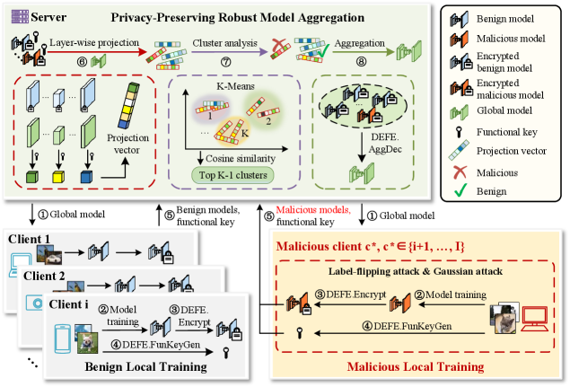
Figure 1: The workflow of SRFed.
V-A High-Level Description of SRFed
The workflow of SRFed is illustrated in Figure 1. Specifically, SRFed iteratively performs the following three steps: 1) Initialization. The server initializes the global model $W_{0}$ and distributes it to all clients (step ①). 2) Local training. In the $t$ -th training iteration, each client $C_{i}$ receives the global model $W_{t}$ from the server and performs local training on its private dataset to obtain the local model $W_{t}^{i}$ (step ②). To protect model privacy, $C_{i}$ encrypts the local model and gets the encrypted model $E_{t}^{i}$ (step ③). Then, $C_{i}$ generates the functional key $skf_{t}^{i}$ for model detection (step ④), and uploads the encrypted model and the functional key to the server (step ⑤). 3) Privacy-preserving robust model aggregation. Upon receiving all encrypted local models $\{E_{t}^{i}\}_{i=1,...,I}$ , the server computes a layer-wise projection vector $V_{t}^{i}$ for each model based on the global model $W_{t}$ (step ⑥). The server then performs clustering analysis on $\{V_{t}^{i}\}_{i=1,...,I}$ to filter malicious models and identify benign models (step ⑦). Finally, the server aggregates these benign clients to update the global model $W_{t+1}$ (step ⑧).
V-B Construction of SRFed
V-B 1 Initialization
In this phase, the server first executes the $\textbf{DEFE.Setup}(1^{\lambda},X,$ $Y)$ algorithm to generate the public parameters $pp$ , which are then made publicly available. Each client $C_{i}$ ( $i∈[1,I]$ ) subsequently generates its key pair $(pk_{i},sk_{i})$ by executing the $\textbf{DEFE.KeyGen}(1^{\lambda},N,g)$ algorithm. Finally, the server distributes the initial global model $W_{0}$ to all clients.
V-B 2 Local Training
The local training phase consists of three components: model training, model encryption, and functional key generation. 1) Model Training: In the $t$ -th ( $t∈[1,T]$ ) training round, once receiving the global model $W_{t}$ , each client $C_{i}$ utilizes its local dataset $D_{i}$ to update $W_{t}$ and obtains model update $W_{t}^{i}$ . For benign clients, they minimize their local objective function $L_{i}$ to obtain $W_{t}^{i}$ , i.e.,
$$
W_{t}^{i}=\arg\min_{W_{t}}L_{i}(W_{t},D_{i}). \tag{4}
$$
Malicious clients execute distinct update strategies based on their attack method. Specifically, to perform a Gaussian attack, malicious clients first conduct normal local training according to Equation (4) to obtain the benign model $W_{t}^{i}$ , and subsequently inject Gaussian noise $noise_{t}$ into it to produce a poisoned model $(W_{t}^{i})^{*}$ , i.e.,
$$
(W_{t}^{i})^{*}=W_{t}^{i}+noise_{t}. \tag{5}
$$
In addition, to launch a label-flipping attack, malicious clients first poison their training datasets by flipping all samples labeled as $l_{\text{src}}$ to a target class $l_{\text{tar}}$ . They then perform local training on the poisoned dataset $D_{i}^{*}(l_{\text{src}}→ l_{\text{tar}})$ to derive the poisoned model $(W_{t}^{i})^{*}$ , i.e.,
$$
(W_{t}^{i})^{*}=\arg\min_{W_{t}^{i}}L_{i}\left(W_{t}^{i},D_{i}^{*}(l_{\text{src}}\rightarrow l_{\text{tar}})\right). \tag{6}
$$
2) Model Encryption: To protect the privacy information of the local model, the clients exploit the DEFE scheme to encrypt their local models. Specifically, the clients first parse the local model as $W_{t}^{i}=[W_{t}^{(i,1)},...,W_{t}^{(i,l)},...,W_{t}^{(i,L)}]$ , where $W_{t}^{(i,l)}$ denotes the parameter set of the $l$ -th model layer. For each parameter element $W_{t}^{(i,l)}[\varepsilon]$ in $W_{t}^{(i,l)}$ , client $C_{i}$ executes the $\textbf{DEFE.Encrypt}(pk_{i},sk_{i},ctr,W_{t}^{(i,l)}[\varepsilon])$ algorithm to generate the encrypted parameter $E_{t}^{(i,l)}[\varepsilon]$ , i.e.,
$$
E_{t}^{(i,l)}[\varepsilon]=(1+N)^{{W_{t}^{(i,l)}}^{\prime}[\varepsilon]}\cdot g^{{r_{i}}^{ctr}}\bmod N^{2}, \tag{7}
$$
where ${W_{t}^{(i,l)}}^{\prime}[\varepsilon]$ is the parameter $W_{t}^{(i,l)}[\varepsilon]$ perturbed by a noise term $\eta$ , i.e.,
$$
{W_{t}^{(i,l)}}^{\prime}[\varepsilon]=W_{t}^{(i,l)}[\varepsilon]+\eta. \tag{8}
$$
In SRFed, the noise $\eta$ remains fixed for all clients during the first $T-1$ training rounds, and is set to $0$ in the final training round. Specifically, $\eta$ is an integer generated by client $C_{1}$ using the hash function $H_{1}$ during the first iteration, and is subsequently broadcast to all other clients for model encryption. The magnitude of $\eta$ is constrained by:
$$
m_{l}\cdot\eta^{2}\ll\lVert W_{0}^{(l)}\rVert^{2},\quad\forall l\in[1,L], \tag{9}
$$
where $W_{0}^{(l)}$ denotes the $l$ -th layer model parameters of the initial global model $W_{0}$ , and $m_{l}$ represents the number of parameters in $W_{0}^{(l)}$ . Finally, the client $C_{i}$ obtains the encrypted local model $E_{t}^{i}=[E_{t}^{(i,1)},...,E_{t}^{(i,l)},...,E_{t}^{(i,L)}]$ .
3) Functional Key Generation: Each client $C_{i}$ generates a functional key vector $skf_{t}^{i}=[skf_{t}^{(i,1)},skf_{t}^{(i,2)},...,skf_{t}^{(i,L)}]$ to enable the server to perform model detection on encrypted models. Specifically, for the $l$ -th layer of the global model $W_{t}$ , client $C_{i}$ executes the $\textbf{DEFE.FunKeyGen}(pk_{i},sk_{i},ctr,W_{t}^{(l)}[\varepsilon])$ algorithm to generate element-wise functional keys, i.e.,
$$
skf_{t}^{(i,l,\varepsilon)}=r_{i}^{ctr}\cdot W_{t}^{(l)}[\varepsilon]=H_{1}(sk_{i},ctr,\varepsilon)\cdot W_{t}^{(l)}[\varepsilon], \tag{10}
$$
where $W_{t}^{(l)}[\varepsilon]$ denotes the $\varepsilon$ -th parameter of $W_{t}^{(l)}$ . After processing all elements in $W_{t}^{(l)}$ , client $C_{i}$ obtains the set of element-wise functional keys $\{\{skf_{t}^{(i,l,\varepsilon)}\}_{\varepsilon=1}^{|W_{t}^{(l)}|}\}_{l=1}^{L}$ . Subsequently, the layer-level functional key is derived by aggregating the element-wise keys using the $\textbf{DEFE.FunKeyAgg}(\{skf_{t}^{(i,l,\varepsilon)}\}_{\varepsilon=1}^{|W_{t}^{(l)}|})$ algorithm, i.e.,
$$
skf_{t}^{(i,l)}=\sum\nolimits_{\varepsilon=1}^{|W_{t}^{(l)}|}skf_{t}^{(i,l,\varepsilon)}. \tag{11}
$$
This procedure is repeated for all layers to obtain the complete functional key vector $skf_{t}^{i}$ for client $C_{i}$ . Finally, each client uploads the encrypted local model $E_{t}^{i}$ and the corresponding functional key $skf_{t}^{i}$ to the server for subsequent model detection and aggregation.
V-B 3 Privacy-Preserving Robust Model Aggregation
To resist poisoning attacks from malicious clients, SRFed implements a privacy-preserving robust aggregation strategy, which enables secure detection and aggregation of encrypted local models without exposing private information. As illustrated in Figure 1, the proposed method performs layer-wise projection and clustering analysis to identify abnormal updates and ensure reliable model aggregation. Specifically, in each training round, the local model $W_{t}^{i}$ and the global model $W_{t}$ are decomposed layer by layer. For each layer, the parameters are projected onto the corresponding layer of the global model, and clustering is performed on the projection vectors to detect anomalous models. After that, the server filters malicious models and aggregates the remaining benign updates. Unlike prior defenses that rely on global statistical similarity between model updates [33, 29, 35], our approach captures fine-grained parameter anomalies and conducts clustering analysis to achieve effective detection even under non-IID data distributions.
1) Model Detection: Once receiving $E_{t}^{i}$ and $skf_{t}^{i}$ from client $C_{i}$ , the server computes the projection $V_{t}^{(i,l)}$ of $W_{t}^{(i,l)^{\prime}}$ onto $W_{t}^{(l)}$ , i.e.,
$$
V_{t}^{(i,l)}=\frac{\langle W_{t}^{(i,l)^{\prime}},W_{t}^{(l)}\rangle}{\lVert W_{t}^{(l)}\rVert_{2}}. \tag{12}
$$
Specifically, the server first executes the $\textbf{DEFE.AggDec}(skf_{t}^{(i,l)},$ $E_{t}^{(i,l)})$ algorithm, which effectively computes the inner product of $W_{t}^{(i,l)^{\prime}}$ and $W_{t}^{(l)}$ . This value is then normalized by $\lVert W_{t}^{(l)}\rVert_{2}$ to obtain
$$
V_{t}^{(i,l)}=\frac{\textbf{DEFE.AggDec}(skf_{t}^{(i,l)},E_{t}^{(i,l)})}{\lVert W_{t}^{(l)}\rVert_{2}}. \tag{13}
$$
By iterating over all $L$ layers, the server obtains the layer-wise projection vector $V_{t}^{i}=[V_{t}^{(i,1)},V_{t}^{(i,2)},...,V_{t}^{(i,L)}]$ corresponding to client $C_{i}$ . After computing projection vectors for all clients, the server clusters the set $\{V_{t}^{i}\}_{i=1}^{I}$ into $K$ clusters $\{\Omega_{1},\Omega_{2},...,\Omega_{K}\}$ using the K-Means algorithm. For each cluster $\Omega_{k}$ , the centroid vector $\bar{V}_{k}$ is computed, and the average cosine similarity $\overline{cs}_{k}$ between all vectors in the cluster and $\bar{V}_{k}$ is calculated. Finally, the $K-1$ clusters with the largest average cosine similarities are identified as benign clusters, while the remaining cluster is considered potentially malicious.
3) Model Aggregation: The server first maps the vectors in the selected $K-1$ clusters to their corresponding clients, generating a client list $L^{t}_{bc}$ and a weight vector $\gamma_{t}=(\gamma^{1}_{t},...,\gamma^{I}_{t})$ , where
$$
\gamma^{i}_{t}=\begin{cases}1&\text{if }C_{i}\in L^{t}_{bc},\\
0&\text{otherwise.}\end{cases} \tag{14}
$$
The server then distributes $\gamma_{t}$ to all clients. Upon receiving $\gamma^{i}_{t}$ , each client $C_{i}$ locally executes the $\textbf{DEFE.FunKeyGen}(pk_{i},sk_{i},$ $ctr,\gamma^{i}_{t},aux)$ algorithm to compute the partial functional key $skf^{(i,\mathsf{Agg})}_{t}$ as
$$
skf^{(i,\mathsf{Agg})}_{t}=r_{i}^{ctr}y^{i}_{t}+\sum_{j=1}^{i-1}\varphi^{i,j}-\sum_{j=i+1}^{n}\varphi^{i,j}. \tag{15}
$$
Each client uploads $skf^{(i,\mathsf{Agg})}_{t}$ to the server. Subsequently, the server executes the $\textbf{DEFE.FunKeyAgg}\left((skf^{(i,\mathsf{Agg})}_{t})_{i=1}^{I}\right)$ to compute the aggregation key as
$$
skf^{\mathsf{Agg}}_{t}=\sum_{i=1}^{I}skf^{(i,\mathsf{Agg})}_{t}. \tag{16}
$$
Finally, the server performs layer-wise aggregation to obtain the noise-perturbed global model $W_{t+1}^{\prime}$ as
$$
\displaystyle W_{t+1}^{(l)^{\prime}}[\varepsilon] \displaystyle=\frac{\text{DEFE.AggDec}\left(skf^{\mathsf{Agg}}_{t},\{E_{t}^{(i,l)}[\varepsilon]\}_{i=1}^{I}\right)}{n} \displaystyle=\frac{\langle(W_{t}^{(1,l)^{\prime}}[\varepsilon],\dots,W_{t}^{(I,l)^{\prime}}[\varepsilon]),\gamma_{t}\rangle}{n} \tag{17}
$$
where $n$ denotes the number of 1-valued elements in $L^{t}_{bc}$ . The server then distributes $W_{t+1}^{\prime}$ to all clients for the $(t+1)$ -th training round. Note that $W_{t+1}^{\prime}$ is noise-perturbed, the clients must remove the perturbation to recover the accurate global model $W_{t+1}$ . They will execute the $\textbf{DEFE.UsrDec}(W_{t+1}^{(l)^{\prime}}[\varepsilon],\gamma_{t})$ algorithm to restore the true global model parameter $W_{t+1}^{(l)}[\varepsilon]=W_{t+1}^{(l)^{\prime}}[\varepsilon]-\eta$ .
VI Analysis
VI-A Confidentiality
In this subsection, we demonstrate that our DEFE-based SRFed framework guarantees the confidentiality of clients’ local models under the Honest-but-Curious (HBCS) security setting.
**Definition VI.1 (Decisional Composite Residuosity (DCR) Assumption[43])**
*Selecting safe primes $p=2p^{\prime}+1$ and $q=2q^{\prime}+1$ with $p^{\prime},q^{\prime}>2^{l(\lambda)}$ , where $l$ is a polynomial in security parameter $\lambda$ , let $N=pq$ . The Decision Composite Residuosity (DCR) assumption states that, for any Probability Polynomial Time (PPT) adversary $\mathcal{A}$ and any distinct inputs $x_{0},x_{1}$ , the following holds:
$$
|Pr_{win}(\mathcal{A},(1+N)^{x_{0}}\cdot g^{r_{i}^{ctr}}\mod N^{2},x_{0},x_{1})-\frac{1}{2}|=negl(\lambda),
$$
where $Pr_{win}$ denotes the probability that the adversary $\mathcal{A}$ distinguishes ciphertexts.*
**Definition VI.2 (Honest but Curious Security (HBCS))**
*Consider the following game between an adversary $\mathcal{A}$ and a PPT simulator $\mathcal{A}^{*}$ , a protocol $\Pi$ is secure if the real-world view $\textbf{REAL}_{\mathcal{A}}^{\Pi}$ of $\mathcal{A}$ is computationally indistinguishable from the ideal-world view $\textbf{IDEAL}_{\mathcal{A}^{*}}^{\mathcal{F_{\Pi}}}$ of $\mathcal{A}^{*}$ , i.e., for all inputs $\hat{x}$ and intermediate results $\hat{y}$ from participants, it holds $\textbf{REAL}_{\mathcal{A}}^{\Pi}(\lambda,\hat{x},\hat{y})\overset{c}{\equiv}\textbf{IDEAL}_{\mathcal{A}^{*}}^{\mathcal{F_{\Pi}}}(\lambda,\hat{x},\hat{y})$ , where $\overset{c}{\equiv}$ denotes computationally indistinguishable.*
**Theorem VI.1**
*SRFed achieves Honest but Curious Security under the DCR assumption, which means that for all inputs $\{C_{t}^{i},{skf}_{t}^{i}\}_{i=1,...,I}$ and intermediate results ( $V_{t}^{i}$ , $W_{t+1}^{\prime}$ , $W_{T}$ ), SRFed holds: $\textbf{REAL}_{\mathcal{A}}^{SRFed}(C_{t}^{i},{skf}_{t}^{i},skf_{t}^{\mathsf{Agg}},V_{t}^{i},W_{t+1}^{\prime},W_{T})\overset{c}{\equiv}$ $\textbf{IDEAL}_{\mathcal{A}^{*}}^{\mathcal{F}_{SRFed}}(C_{t}^{i},{skf}_{t}^{i},skf_{t}^{\mathsf{Agg}},V_{t}^{i},W_{t+1}^{\prime},W_{T})$ .*
* Proof:*
To prove the security of SRFed, we just need to prove the confidentiality of the privacy-preserving defense strategy, since only it involves the computation of private data by unauthorized entities (i.e., the server). For the curious server, $\textbf{REAL}_{\mathcal{A}}^{SRFed}$ contains intermediate parameters and encrypted local models $\{C_{t}^{i}\}_{i=1,...,I}$ collected from each client during the execution of SRFed protocols. Besides, we construct a PPT simulator $\mathcal{A}^{*}$ to execute $\mathcal{F}_{SRFed}$ , which simulates each process of the privacy-preserving defensive aggregation strategy. The detailed proof is described below. Hyb 1 We initialize a series of random variables whose distributions are indistinguishable from $\textbf{REAL}_{\mathcal{A}}^{SRFed}$ during the real protocol execution. Hyb 2 In this hybrid, we change the behavior of simulated client $C_{i}$ $(i∈[1,I])$ . $C_{i}$ takes the selected random vector of random variables $\Theta_{W}$ as the local model $W_{t}^{i^{\prime}}$ , and uses the DEFE.Encrypt algorithm to encrypt $W_{t}^{i^{\prime}}$ . As only the original contents of ciphertexts have changed, it guarantees that the server cannot distinguish the view of $\Theta_{W}$ from the view of original $W_{t}^{i^{\prime}}$ according to the Definition (VI.1). Then, $C_{i}$ uses the DEFE.FunKeyGen algorithm to generate the key vector $skf_{t}^{i}=[skf_{t}^{(i,1)},skf_{t}^{(i,2)},...,skf_{t}^{(i,L)}].$ Note that each component of $skf_{t}^{i}$ essentially is the inner product result, thus revealing no secret information to the server. Hyb 3 In this hybrid, we change the input of the protocol of Secure Model Aggregation executed by the server with encrypted random variables instead of real encrypted model parameters. The server gets the plaintexts vector $V_{t}^{i}=[V_{t}^{(i,1)},V_{t}^{(i,2)},...,V_{t}^{(i,L)}]$ corresponding to $C_{i}$ , which is the layer-wise projection of $\Theta_{W}$ and $W_{t}$ . As the inputs $\Theta_{W}$ follow the same distribution as the real $W^{i^{\prime}}_{t}$ , the server cannot distinguish the $V_{t}^{i}$ between ideal world and real world without knowing further information about the inputs. Then, the server performs clustering based on $\{V_{t}^{i}\}^{I}_{i=1}$ to obtain $\{\Omega_{k}\}^{K}_{k=1}$ . Subsequently, it computes the average cosine similarity of all vectors within each cluster to their centroid, and assigns client weights accordingly. Since $\{V_{t}^{i}\}^{I}_{i=1}$ is indistinguishable between the ideal world and the real world, the intermediate variables calculated via $\{V_{t}^{i}\}^{I}_{i=1}$ above also inherit this indistinguishability. Hence, this hybrid is indistinguishable from the previous one. Hyb 4 In this hybrid, the aggregated model $W_{t+1}^{\prime}$ is computed by the DEFE.AggDec algorithm. $\mathcal{A}^{*}$ holds the view $\textbf{IDEAL}_{\mathcal{A}^{*}}^{\mathcal{F}_{SRFed}}$ $=$ $(C_{t}^{i},{skf}_{t}^{i},skf_{t}^{\mathsf{Agg}},V_{t}^{i},W_{t+1}^{\prime},W_{T})$ , where $skf_{t}^{\mathsf{Agg}}$ is obtained by the interaction of non-colluding clients and server, the full security property of DEFE and the non-colluding setting ensure the security of $skf_{t}^{\mathsf{Agg}}$ . Among the elements of intermediate computation, the local model $W_{t}^{i^{\prime}}$ is encrypted, which is consistent with the previous hybrid. Throughout the $T$ -round iterative process, the server obtains the noise-perturbed aggregated model $W_{t+1}^{\prime}=W_{t+1}+\eta$ via the secure model aggregation when $0≤ t<T-1$ . Thus, the server cannot infer the real $W_{t+1}$ , and cannot distinguish the $W_{t+1}^{\prime}$ between ideal world and real world. When $t=T-1$ , since the distribution of $\Theta_{W}$ remains identical to that of $W_{T}$ , the probability that the server can distinguish the final averaged aggregated model $W_{T}$ is negligible. Hence, this hybrid is indistinguishable from the previous one. Hyb 5 When $0≤ t<T$ , all clients further execute the DEFE.UsrDec algorithm to restore the $W_{t+1}$ . This process is independent of the server, hence this hybrid is indistinguishable from the previous one. The argument above proves that the output of $\textbf{IDEAL}_{\mathcal{A}^{*}}^{\mathcal{F}_{SRFed}}$ is indistinguishable from the output of $\textbf{REAL}_{\mathcal{A}}^{SRFed}$ . Thus, it proves that SRFed guarantees HBCS. ∎
VI-B Robustness
To theoretically analyze the robustness of SRFed against poisoning attacks, we first prove the following theorem.
**Theorem VI.2**
*When the noise perturbation $\eta$ satisfies the constraint in (9), the clustering results of SRFed over all $T$ iterations remain approximately equivalent to those obtained using the original local models $\{W_{t}^{i}\}_{1,2,...,I}$ .*
* Proof:*
Let $\overline{\eta}$ be a vector of the same shape as $W_{t}^{(i,l)^{\prime}}$ with all entries equal to $\eta$ , and ${V_{t}^{i}}_{real}$ be the real projection vector derived from the noise-free models. We discuss the following three cases. ① $t=0:$ For any $i∈[1,I]$ , $W_{0}^{(i,l)^{\prime}}=W_{0}^{(i,l)}+\overline{\eta}$ , we have
$$
\displaystyle V_{0}^{i} \displaystyle=\frac{\langle W_{0}^{(i,l)^{\prime}},W_{0}^{(l)}\rangle}{\lVert W_{0}^{(l)}\rVert_{2}}=\frac{\langle W_{0}^{(i,l)}+\overline{\eta},W_{0}^{(l)}\rangle}{\lVert W_{0}^{(l)}\rVert_{2}}={V_{0}^{i}}_{real}+\frac{\langle\overline{\eta},W_{0}^{(l)}\rangle}{\lVert W_{0}^{(l)}\rVert_{2}}. \tag{18}
$$
Note that $\frac{\langle\overline{\eta},W_{0}^{(l)}\rangle}{\lVert W_{0}^{(l)}\rVert_{2}}$ is identical for any client, the clustering result of $\{V_{0}^{i}\}^{I}_{i=1}$ is entirely equivalent to that of $\{{V_{0}^{i}}_{real}\}^{I}_{i=1}$ based on the underlying computation of K-Means. ② $0<t<T:$ For any $i∈[1,I]$ , $W_{t}^{(i,l)^{\prime}}=W_{t}^{(i,l)}+\overline{\eta}$ . Correspondingly, $W_{t}^{(l)^{\prime}}=W_{t}^{(l)}+\overline{\eta}$ , and we have
$$
\begin{split}V_{t}^{i}&=\frac{\langle W_{t}^{(i,l)^{\prime}},W_{t}^{(l)^{\prime}}\rangle}{\lVert W_{t}^{(l)^{\prime}}\rVert_{2}}\\
&=\frac{\langle W_{t}^{(i,l)},W_{t}^{(l)}\rangle+\langle W_{t}^{(i,l)},\overline{\eta}\rangle+\langle\overline{\eta},W_{t}^{(l)}\rangle+\langle\overline{\eta},\overline{\eta}\rangle}{\sqrt[]{\lVert W_{t}^{(l)}\rVert_{2}^{2}+2\langle W_{t}^{(l)},\overline{\eta}\rangle+\lVert\overline{\eta}\rVert_{2}^{2}}}.\end{split} \tag{19}
$$
By combining the above equation with the constraint (9), $V_{t}^{i}$ is approximately equivalent to the real value of ${V_{t}^{i}}_{real}$ . ③ $t=T:$ For any $i∈[1,I]$ , $W_{T}^{(i,l)^{\prime}}=W_{T}^{(i,l)}$ . Correspondingly, $W_{T}^{(l)^{\prime}}=W_{T}^{(l)}+\overline{\eta}$ , and we have
$$
\displaystyle V_{T}^{i} \displaystyle=\frac{\langle W_{T}^{(i,l)},W_{T}^{(l)^{\prime}}\rangle}{\lVert W_{T}^{(l)^{\prime}}\rVert_{2}}=\frac{\langle W_{T}^{(i,l)},W_{T}^{(l)}\rangle+\langle W_{T}^{(i,l)},\overline{\eta}\rangle}{\sqrt[]{\lVert W_{T}^{(l)}\rVert_{2}^{2}+2\langle W_{T}^{(l)},\overline{\eta}\rangle+\lVert\overline{\eta}\rVert_{2}^{2}}}. \tag{20}
$$
Similarly, by combining the above equation with the constraint (9), $V_{T}^{i}$ is approximately equivalent to the real value of ${V_{T}^{i}}_{real}$ . Therefore, across all iterations, the clustering results based on $\{V_{t}^{i}\}$ closely approximate those derived from the original local models, confirming that the introduced perturbation does not affect model detection. ∎
Then, we introduce a key assumption, which has been proved in [37, 32]. This assumption reveals the essential difference between malicious and benign models and serves as a core basis for subsequent robustness analysis.
**Assumption VI.1**
*An error term $\tau^{(t)}$ exists between the average malicious gradients $\mathbf{W}_{t}^{i*}$ and the average benign gradients $\mathbf{W}_{t}^{i}$ due to divergent training objectives. This is formally expressed as:
$$
\sum_{C_{i}\in\mathcal{M}}\mathbf{W}_{t}^{i*}=\sum_{C_{i}\in\mathcal{B}}\mathbf{W}_{t}^{i}+\tau^{(t)}. \tag{21}
$$
The magnitude of $\tau^{(t)}$ exhibits a positive correlation with the number of iterative training rounds.*
**Theorem VI.3**
*SRFed guarantees robustness to malicious clients in non-IID settings, provided that most clients are benign.*
* Proof:*
In the secure model aggregation phase of SRFed, the server collects the encrypted model $C_{t}^{i}$ and the corresponding key vectors $skf_{t}^{i}$ from each client, then computes the projection $V_{t}^{(i,l)}$ of $W_{t}^{(i,l)}$ onto $W_{t}^{(l)}$ , i.e., $\frac{\langle W_{t}^{(i,l)},W_{t}^{(l)}\rangle}{\lVert W_{t}^{(l)}\rVert_{2}}$ . By iterating over $L$ layers, the server obtains the layer-wise projection vector $V_{t}^{i}=[V_{t}^{(i,1)},V_{t}^{(i,2)},...,V_{t}^{(i,L)}]$ corresponding to $C_{i}$ . Subsequently, the server performs clustering on the projection vectors $\{V_{t}^{i}\}^{I}_{i=1}$ . Based on the Assumption (VI.1), a non-negligible divergence $\tau^{(t)}$ emerges between benign and malicious local models, which grows with the number of iterations. Meanwhile, by independently projecting each layer’s parameters onto the corresponding layer of the global model, our operation eliminates cross-layer interference. This ensures that malicious modifications confined to specific layers can be detected significantly more effectively. Therefore, our clustering approach successfully distinguishes between benign and malicious models by grouping them into separate clusters. Due to significant distribution divergence, malicious models exhibit a lower average cosine similarity to their cluster center. Consequently, our scheme filters out the cluster containing malicious models by computing average cosine similarity, ultimately achieving robust to malicious clients. ∎
VI-C Efficiency
**Theorem VI.4**
*The computation and communication complexities of SRFed are $\mathcal{O}(T_{lt})+\mathcal{O}(\zeta T_{me-defe})+\mathcal{O}(T_{md-defe})+\mathcal{O}(T_{ma-defe})$ and $\mathcal{O}(I\zeta|w_{defe}|)+\mathcal{O}(IL|w|)$ , respectively.*
* Proof:*
To evaluate the efficiency of SRFed, we analyze its computational and communication overhead per training iteration and compare it with ShieldFL [29]. ShieldFL is an efficient PPFL framework based on the partially homomorphic encryption (PHE) scheme. The comparative results are presented in Table III. Specifically, the computational overhead of SRFed comprises four components: local training $\mathcal{O}(T_{lt})$ , model encryption $\mathcal{O}(\zeta T_{me-defe})$ , model detection $\mathcal{O}(T_{md-defe})$ , and model aggregation $\mathcal{O}(T_{ma-defe})$ . For model encryption, FE inherently offers a lightweight advantage over PHE, leading to $\mathcal{O}(\zeta T_{me-defe})<\mathcal{O}(\zeta T_{me-phe})$ . In terms of model detection, SRFed performs this process primarily on the server side using plaintext data, whereas ShieldFL requires multiple rounds of interaction to complete the encrypted model detection. This results in $\mathcal{O}(T_{md-defe})\ll\mathcal{O}(T_{md-phe})$ . Furthermore, SRFed enables the server to complete decryption and aggregation simultaneously. In contrast, ShieldFL necessitates aggregation prior to decryption and involves interactions with a third party, resulting in significantly higher overhead, i.e., $\mathcal{O}(T_{ma-defe})\ll\mathcal{O}(T_{ma-phe})$ . Overall, these characteristics collectively render SRFed more efficient than ShieldFL. The communication overhead of SRFed comprises two components: the encrypted models $\mathcal{O}(I\zeta|w_{defe}|)$ and key vectors $\mathcal{O}(IL|w|)$ uploaded by $I$ clients, where $\zeta$ denotes the model dimension, $L$ is the number of layers, $|w_{defe}|$ and $|w|$ are the communication complexity of a single DEFE ciphertext and a single plaintext, respectively. Since $|w|$ is significantly lower than $|w_{defe}|$ , and $|w_{defe}|$ and $|w_{phe}|$ are nearly equivalent, SRFed reduces the overall communication complexity by approximately $\mathcal{O}(12I\zeta|w_{phe}|)$ compared to ShieldFL. This reduction in overhead is primarily attributed to SRFed’s lightweight DEFE scheme, which eliminates extensive third-party interactions. ∎
TABLE III: Comparison of computation and communication overhead between different methods
| Method | SRFed | ShieldFL |
| --- | --- | --- |
| Comp. | $\mathcal{O}(T_{lt})+\mathcal{O}(\zeta T_{me-defe})$ | $\mathcal{O}(T_{lt})+\mathcal{O}(\zeta T_{me-phe})$ |
| $+\mathcal{O}(T_{ma-defe})$ | $+\mathcal{O}(\zeta T_{md-phe})$ | |
| $+\mathcal{O}(T_{ma-defe})$ | $+\mathcal{O}(T_{md-phe})$ | |
| Comm. | $\mathcal{O}(I\zeta|w_{defe}|)^{1}+\mathcal{O}(IL|w|)^{2}$ | $\mathcal{O}(13I\zeta|w_{phe}|)^{\mathrm{3}}$ |
- Notes: ${}^{\mathrm{1,2,3}}|w_{defe}|$ , $|w|$ and $|w_{phe}|$ denote the communication complexity of a DEFE ciphertext, a plaintext, and a PHE ciphertext, respectively.
VII Experiments
VII-A Experimental Settings
VII-A 1 Implementation
We implement SRFed on a small-scale local network. Each machine in the network is equipped with the following hardware configuration: an Intel Xeon CPU E5-1650 v4, 32 GB of RAM, an NVIDIA GeForce GTX 1080 Ti graphics card, and a network bandwidth of 40 Mbps. Additionally, the implementation of the DEFE scheme is based on the NDD-FE scheme [31], and the code implementation of FL processes is referenced to [44].
VII-A 2 Dataset and Models
We evaluate the performance of SRFed on two datasets:
- MNIST [45]: This dataset consists of 10 classes of handwritten digit images, with 60,000 training samples and 10,000 test samples. Each sample is a grayscale image of 28 × 28 pixels. The global model used for this dataset is a Convolutional Neural Network (CNN) model, which includes two convolutional layers followed by two fully connected layers.
- CIFAR-10 [46]: This dataset contains RGB color images across 10 categories, including airplane, car, bird, cat, deer, dog, frog, horse, boat, and truck. It consists of 50,000 training images and 10,000 test samples. Each sample is a 32 × 32 pixel color image. The global model used for this dataset is a CNN model, which includes three convolutional layers, one pooling layer, and two fully connected layers.
VII-A 3 Baselines
To evaluate the robustness of the proposed SRFed method, we conduct comparative experiments against several advanced baseline methods, including FedAvg [47], ShieldFL [29], PBFL [37], Median [35], Biscotti [41], and FoolsGold [33]. Furthermore, to evaluate the efficiency of SRFed, we compare it with representative methods such as ShieldFL [29] and ESB-FL [31].
VII-A 4 Experimental parameters
In all experiments, the number of local clients is set to 20, the number of training rounds is set to 100, the batchsize is set to 64, and the number of local training epochs is set to 10. We use the stochastic gradient descent (SGD) to optimize the model, with a learning rate of 0.01 and a momentum of 0.5. Additionally, our experiments are conducted under varying levels of data heterogeneity, with the data distributions configured as follows:
- MNIST: Two distinct levels of data heterogeneity are configured by sampling from a Dirichlet distribution with the parameters $\alpha=0.2$ and $\alpha=0.8$ , respectively, to simulate Non-IID data partitions across clients.
- CIFAR-10: Two distinct levels of data heterogeneity are configured by sampling from a Dirichlet distribution with the parameters $\alpha=0.2$ and $\alpha=0.6$ , respectively, to simulate Non-IID data partitions across clients.
VII-A 5 Attack Scenario
In each benchmark, the adversary can control a certain proportion of clients to launch poisoning attacks, with the proportion varying across {0%, 10%, 20%, 30%, 40%, 50%}. The attack scenario parameters are configured as follows:
- Targeted Poisoning Attack: we consider the mainstream label-flipping attack. For experiments on the MNIST dataset, the training samples originally labeled as ”0” are reassigned to the target label ”4”. For the CIFAR-10 dataset, the training samples originally labeled as ”airplane” are reassigned to the target label ”deer”.
- Untargeted Poisoning Attack: We consider the commonly used Gaussian attack. In experiments, malicious clients inject noise that follows a Gaussian distribution $\mathcal{N}(0,0.5^{2})$ into their local model updates.
VII-A 6 Evaluation Metrics
For each benchmark experiment, we adopt the following evaluation metrics on the test dataset to quantify the impact of poisoning attacks on the aggregated model in FL.
- Overall Accuracy (OA): It is the ratio of the number of samples correctly predicted by the model in the test dataset to the total number of predictions for all samples in the test dataset.
- Source Accuracy (SA): It specifically refers to the ratio of the number of correctly predicted flip class samples by the model to the total number of flip class samples in the dataset.
- Attack Success Rate (ASR): It is defined as the proportion of source-class samples that are misclassified as the target class by the aggregated model.
<details>
<summary>x2.png Details</summary>
### Visual Description
## Line Chart: Accuracy vs. Attack Ratio
### Overview
The chart compares the accuracy retention of various machine learning defense mechanisms against adversarial attacks, measured as attack ratio percentage. Accuracy is plotted on the y-axis (84-96%) and attack ratio on the x-axis (0-50%). Seven defense strategies are compared through distinct colored lines with unique markers.
### Components/Axes
- **Y-axis**: Accuracy (%) [84-96], labeled "Accuracy (%)"
- **X-axis**: Attack ratio (%) [0-50], labeled "Attack ratio (%)"
- **Legend**: Located in bottom-left corner, mapping:
- Blue squares: FedAvg
- Orange diamonds: ShieldFL
- Green triangles: PBFL
- Purple diamonds: Median
- Gray stars: Biscotti
- Brown triangles: FoolsGold
- Red circles: Ours
### Detailed Analysis
1. **FedAvg** (blue squares): Starts at ~96.5% accuracy at 0% attack ratio, shows gradual decline to ~95.5% at 50% attack ratio.
2. **ShieldFL** (orange diamonds): Begins at ~96.2%, maintains near-horizontal trajectory until 40% attack ratio, then drops sharply to ~87%.
3. **PBFL** (green triangles): Starts at ~96.3%, shows moderate decline to ~94.5% at 50% attack ratio.
4. **Median** (purple diamonds): Remains relatively flat at ~95.8% across all attack ratios.
5. **Biscotti** (gray stars): Starts at ~96%, shows steep linear decline to ~83.5% at 50% attack ratio.
6. **FoolsGold** (brown triangles): Begins at ~96.1%, maintains stability until 40% attack ratio, then plummets to ~85%.
7. **Ours** (red circles): Maintains highest accuracy throughout, starting at ~96.4% and ending at ~95.8% with minimal decline.
### Key Observations
- **Robustness**: "Ours" demonstrates superior resilience, maintaining >95% accuracy across all attack ratios.
- **Vulnerability**: "Biscotti" and "FoolsGold" exhibit the most severe degradation, dropping >12% accuracy at maximum attack ratio.
- **Stability**: "Median" and "PBFL" show moderate stability, with <2% accuracy loss across the attack spectrum.
- **Threshold Behavior**: "ShieldFL" and "FoolsGold" exhibit threshold-like behavior, maintaining high accuracy until a critical attack ratio (~40%) before rapid decline.
### Interpretation
The data reveals fundamental differences in attack resilience among defense mechanisms. The "Ours" method's consistent performance suggests architectural advantages in adversarial robustness. The sharp declines in "Biscotti" and "FoolsGold" indicate potential single points of failure in their designs. Notably, the "Median" method's stability implies that simple averaging techniques may provide baseline protection against certain attack types. The threshold behavior observed in "ShieldFL" and "FoolsGold" suggests these methods might employ confidence-based filtering mechanisms that become ineffective beyond certain attack intensities. These findings highlight the importance of defense mechanism design in maintaining model utility under adversarial conditions, with "Ours" establishing a new benchmark for attack resilience in this evaluation.
</details>
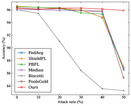
(a) MNIST ( $\alpha$ =0.2)
<details>
<summary>x3.png Details</summary>
### Visual Description
## Line Chart: Accuracy vs. Attack Ratio for Various Federated Learning Methods
### Overview
The chart compares the accuracy retention of seven federated learning methods (FedAvg, ShieldFL, PBFL, Median, Biscotti, FoolsGold, Ours) as the attack ratio increases from 0% to 50%. Accuracy is measured on the y-axis (70–95%), while the x-axis represents attack ratio percentages. The legend on the left maps colors and markers to each method.
### Components/Axes
- **Y-axis**: Accuracy (%) with ticks at 70, 75, 80, 85, 90, 95.
- **X-axis**: Attack ratio (%) with ticks at 0, 10, 20, 30, 40, 50.
- **Legend**: Positioned on the left, with distinct colors and markers for each method:
- FedAvg: Blue square
- ShieldFL: Orange diamond
- PBFL: Green triangle
- Median: Purple pentagon
- Biscotti: Gray star
- FoolsGold: Brown triangle
- Ours: Red circle
### Detailed Analysis
1. **FedAvg (Blue Square)**: Starts at ~95% accuracy at 0% attack ratio, showing a slight decline to ~93% at 50%.
2. **ShieldFL (Orange Diamond)**: Maintains near-constant accuracy (~95%) across all attack ratios.
3. **PBFL (Green Triangle)**: Begins at ~95%, drops sharply to ~90% at 30%, then stabilizes.
4. **Median (Purple Pentagon)**: Remains flat at ~93% accuracy throughout.
5. **Biscotti (Gray Star)**: Starts at ~95%, plummets to ~70% at 30%, then declines further to ~68% at 50%.
6. **FoolsGold (Brown Triangle)**: Declines gradually from ~94% to ~88% over the attack ratio range.
7. **Ours (Red Circle)**: Stays consistently high (~95%) with minimal variation.
### Key Observations
- **Biscotti** exhibits the most drastic performance drop (~25% accuracy loss at 30% attack ratio), suggesting vulnerability to adversarial attacks.
- **ShieldFL** and **Ours** demonstrate the highest robustness, maintaining >94% accuracy even at 50% attack ratio.
- **PBFL** and **FoolsGold** show moderate resilience but degrade significantly after 30% attack ratio.
- **Median** and **FedAvg** exhibit stable but slightly declining trends, indicating moderate robustness.
### Interpretation
The data highlights critical differences in adversarial robustness among federated learning methods. **Biscotti**'s sharp decline suggests it is highly susceptible to attacks, while **ShieldFL** and **Ours** outperform others, potentially due to advanced defense mechanisms. The gradual decline of **FoolsGold** and **PBFL** implies partial mitigation strategies, whereas **Median** and **FedAvg** represent baseline performance. These trends underscore the importance of attack-aware design in federated learning systems, with **Ours** and **ShieldFL** setting a benchmark for resilience. The chart emphasizes trade-offs between model utility and security, guiding future research toward methods that balance both.
</details>
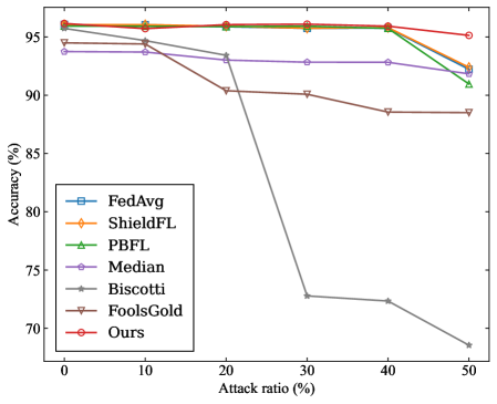
(b) MNIST ( $\alpha$ =0.8)
<details>
<summary>x4.png Details</summary>
### Visual Description
## Line Graph: Accuracy (%) vs Attack ratio (%)
### Overview
The graph compares the accuracy of seven different methods (FedAvg, ShieldFL, PBFL, Median, Biscotti, FoolsGold, Ours) across varying attack ratios (0% to 50%). Accuracy is measured on the y-axis (57.5%–75%), while the x-axis represents the percentage of malicious participants in the system. Each method is represented by a distinct colored line with unique markers.
### Components/Axes
- **X-axis (Attack ratio (%))**: Ranges from 0% to 50% in 10% increments.
- **Y-axis (Accuracy (%))**: Ranges from 57.5% to 75% in 2.5% increments.
- **Legend**: Located at the bottom-left corner, mapping colors/markers to methods:
- **FedAvg**: Blue square
- **ShieldFL**: Orange diamond
- **PBFL**: Green triangle
- **Median**: Purple pentagon
- **Biscotti**: Gray star
- **FoolsGold**: Brown triangle
- **Ours**: Red circle
### Detailed Analysis
1. **FedAvg (Blue Square)**:
- Starts at ~75% accuracy at 0% attack ratio.
- Declines gradually to ~70% at 50% attack ratio.
- Maintains relatively stable performance compared to others.
2. **ShieldFL (Orange Diamond)**:
- Begins at ~75% accuracy at 0%.
- Sharp decline to ~70% by 10% attack ratio.
- Stabilizes slightly above 70% for higher attack ratios.
3. **PBFL (Green Triangle)**:
- Starts at ~74% accuracy at 0%.
- Gradual decline to ~69% at 50%.
- Shows moderate resilience to attacks.
4. **Median (Purple Pentagon)**:
- Begins at ~68% accuracy at 0%.
- Slightly increases to ~69% at 10%, then declines steadily.
- Ends at ~63% at 50%, the lowest among all methods.
5. **Biscotti (Gray Star)**:
- Starts at ~73% accuracy at 0%.
- Sharp decline to ~62% by 20% attack ratio.
- Continues dropping to ~57% at 50%, the steepest slope.
6. **FoolsGold (Brown Triangle)**:
- Begins at ~73% accuracy at 0%.
- Gradual decline to ~68% at 30%.
- Accelerates downward to ~62% at 50%.
7. **Ours (Red Circle)**:
- Starts at ~75% accuracy at 0%.
- Moderate decline to ~70% at 30%.
- Stabilizes near 70% for higher attack ratios, outperforming most methods.
### Key Observations
- **Best Performance at 0% Attack**: FedAvg, ShieldFL, and Ours all start near 75% accuracy.
- **Worst Performance at 50% Attack**: Biscotti drops to ~57%, while Median hits ~63%.
- **Resilience**: Ours and FedAvg maintain the highest accuracy across all attack ratios.
- **Volatility**: ShieldFL and Biscotti show the most dramatic declines, especially after 10% attack ratio.
### Interpretation
The data suggests that **FedAvg** and **Ours** are the most robust methods, maintaining accuracy above 70% even at 50% attack ratios. **ShieldFL** and **PBFL** offer moderate resilience but degrade significantly under high attack conditions. **Biscotti** and **FoolsGold** are highly vulnerable, with steep accuracy drops. The **Median** line indicates that average client performance is poor under attack, highlighting systemic weaknesses. These trends emphasize the importance of attack-aware design in federated learning systems, with **Ours** and **FedAvg** emerging as the most reliable choices for adversarial environments.
</details>
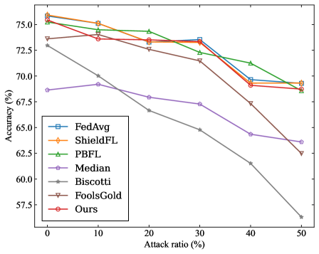
(c) CIFAR10 ( $\alpha$ =0.2)
<details>
<summary>x5.png Details</summary>
### Visual Description
## Line Graph: Accuracy vs. Attack Ratio
### Overview
The graph illustrates the relationship between accuracy (%) and attack ratio (%) for eight different methods. All methods show a general decline in accuracy as the attack ratio increases, with varying degrees of resilience. The legend identifies the methods by color and marker, positioned on the left side of the graph.
### Components/Axes
- **Y-axis**: Accuracy (%) ranging from 62% to 76%.
- **X-axis**: Attack ratio (%) ranging from 0% to 50%.
- **Legend**: Located on the left, with the following mappings:
- **FedAvg**: Blue squares (□)
- **ShieldFL**: Orange diamonds (◇)
- **PBFL**: Green triangles (△)
- **Median**: Purple pentagons (⬡)
- **Biscotti**: Gray stars (★)
- **FoolsGold**: Brown triangles (▼)
- **Ours**: Red circles (●)
### Detailed Analysis
1. **FedAvg (Blue □)**: Starts at ~75.5% accuracy at 0% attack ratio, declining to ~70.5% at 50%.
2. **ShieldFL (Orange ◇)**: Begins at ~75% accuracy, dropping to ~70% at 50%.
3. **PBFL (Green △)**: Starts at ~74.5%, ending at ~70.5%.
4. **Median (Purple ⬡)**: Declines from ~73% to ~68%.
5. **Biscotti (Gray ★)**: Steepest drop from ~74% to ~62.5%.
6. **FoolsGold (Brown ▼)**: Starts at ~75%, ending at ~70%.
7. **Ours (Red ●)**: Declines from ~75.5% to ~72.5%.
### Key Observations
- **Biscotti (Gray ★)** exhibits the most significant decline, losing ~11.5% accuracy over 50% attack ratio.
- **Ours (Red ●)** and **FedAvg (Blue □)** maintain higher accuracy than most methods, with **Ours** showing the smallest drop (~3%).
- **ShieldFL (Orange ◇)** and **FoolsGold (Brown ▼)** have similar trends but **ShieldFL** starts slightly higher.
- **Median (Purple ⬡)** shows a moderate decline (~5%) compared to others.
### Interpretation
The data suggests that **Biscotti** is the least resilient method under increasing attack ratios, while **Ours** and **FedAvg** demonstrate superior robustness. The steep decline in **Biscotti** indicates potential vulnerabilities in its design or implementation. **Ours** and **FedAvg** outperform other methods at higher attack ratios, though **FedAvg** starts with marginally higher initial accuracy. The graph highlights trade-offs between initial performance and resilience, with **Ours** balancing both effectively. The consistent downward trends across all methods underscore the inherent challenge of maintaining accuracy under adversarial conditions.
</details>
(d) CIFAR10 ( $\alpha$ =0.6)
Figure 2: The OA of the models obtained by four benchmarks under label-flipping attack.
<details>
<summary>x6.png Details</summary>
### Visual Description
## Line Chart: Accuracy vs. Attack Ratio for Federated Learning Methods
### Overview
The chart compares the accuracy retention of eight federated learning methods under varying attack ratios (0-50%). Accuracy (%) is plotted on the y-axis (0-100%), while attack ratio (%) is on the x-axis (0-50%). All methods start near 100% accuracy at 0% attack ratio, but performance degrades as attack intensity increases. The red line labeled "Ours" shows the steepest decline, while other methods exhibit more gradual degradation.
### Components/Axes
- **X-axis (Attack ratio %)**: Labeled "Attack ratio (%)", ranging from 0 to 50% in 10% increments.
- **Y-axis (Accuracy %)**: Labeled "Accuracy (%)", ranging from 0 to 100% in 20% increments.
- **Legend**: Positioned in the bottom-left corner, mapping colors/markers to methods:
- Blue square: FedAvg
- Orange diamond: ShieldFL
- Green triangle: PBFL
- Purple circle: Median
- Gray star: Biscotti
- Brown triangle: FoolsGold
- Red circle: Ours
### Detailed Analysis
1. **FedAvg (Blue)**: Starts at ~98% accuracy, declines gradually to ~20% at 50% attack ratio.
2. **ShieldFL (Orange)**: Begins at ~97%, drops to ~30% at 50% attack ratio.
3. **PBFL (Green)**: Maintains ~95% accuracy until 30% attack ratio, then plummets to ~10%.
4. **Median (Purple)**: Declines steadily from ~96% to ~15% at 50% attack ratio.
5. **Biscotti (Gray)**: Drops sharply to 0% accuracy by 30% attack ratio, remaining flat thereafter.
6. **FoolsGold (Brown)**: Declines from ~95% to ~5% at 50% attack ratio.
7. **Ours (Red)**: Starts at ~99%, freefalls to ~70% at 50% attack ratio—the steepest decline among all methods.
### Key Observations
- **Threshold Effect**: All methods experience a critical drop in accuracy after ~30% attack ratio.
- **Resilience Variance**: FedAvg and ShieldFL retain higher accuracy longer than others, suggesting better robustness.
- **Outlier Performance**: "Ours" method (red line) underperforms significantly compared to baselines, with a 29% accuracy loss at 50% attack ratio versus FedAvg’s 78% loss.
- **Biscotti Collapse**: Biscotti (gray line) fails catastrophically at 30% attack ratio, indicating poor attack resilience.
### Interpretation
The data demonstrates that federated learning methods vary widely in their resistance to adversarial attacks. The "Ours" method’s steep decline suggests it may lack effective defense mechanisms compared to established baselines like FedAvg and ShieldFL. The 30% attack ratio threshold appears to be a tipping point where most methods’ defenses fail, though ShieldFL and FedAvg degrade more gradually. Biscotti’s abrupt collapse highlights vulnerabilities in its design. These trends underscore the importance of attack-aware training and robust aggregation protocols in federated learning systems.
</details>
(a) MNIST ( $\alpha$ =0.2)
<details>
<summary>x7.png Details</summary>
### Visual Description
## Line Graph: Accuracy vs. Attack Ratio
### Overview
The image is a line graph comparing the accuracy of eight different methods (FedAvg, ShieldFL, PBFL, Median, Biscotti, FoolsGold, Ours) across varying attack ratios (0% to 50%). Accuracy is measured on the y-axis (0%–100%), while the x-axis represents attack ratio (0%–50%). Each method is represented by a distinct line with unique markers and colors, as indicated in the legend on the left.
### Components/Axes
- **Y-axis**: Accuracy (%)
- Scale: 0% to 100% in 20% increments.
- **X-axis**: Attack ratio (%)
- Scale: 0% to 50% in 10% increments.
- **Legend**:
- **FedAvg**: Blue squares (■)
- **ShieldFL**: Orange diamonds (◆)
- **PBFL**: Green triangles (▲)
- **Median**: Purple circles (●)
- **Biscotti**: Gray stars (★)
- **FoolsGold**: Brown triangles (▼)
- **Ours**: Red circles (○)
### Detailed Analysis
1. **FedAvg (Blue Squares)**:
- Starts at ~98% accuracy at 0% attack ratio.
- Declines gradually to ~62% at 50% attack ratio.
- Slope: Steady downward trend.
2. **ShieldFL (Orange Diamonds)**:
- Starts at ~99% accuracy at 0% attack ratio.
- Declines to ~64% at 50% attack ratio.
- Slope: Moderate downward trend.
3. **PBFL (Green Triangles)**:
- Starts at ~97% accuracy at 0% attack ratio.
- Declines sharply to ~48% at 50% attack ratio.
- Slope: Steep downward trend after 30% attack ratio.
4. **Median (Purple Circles)**:
- Starts at ~96% accuracy at 0% attack ratio.
- Declines slightly to ~90% at 50% attack ratio.
- Slope: Gentle downward trend.
5. **Biscotti (Gray Stars)**:
- Starts at ~99% accuracy at 0% attack ratio.
- Drops catastrophically to ~2% at 30% attack ratio.
- Slope: Vertical collapse at 30% attack ratio.
6. **FoolsGold (Brown Triangles)**:
- Starts at ~98% accuracy at 0% attack ratio.
- Declines to ~38% at 50% attack ratio.
- Slope: Gradual downward trend.
7. **Ours (Red Circles)**:
- Starts at ~99% accuracy at 0% attack ratio.
- Declines minimally to ~96% at 50% attack ratio.
- Slope: Near-flat trend.
### Key Observations
- **Robustness**: Methods like **Ours** and **Median** maintain high accuracy (>90%) even at 50% attack ratio, indicating strong resilience.
- **Vulnerability**: **Biscotti** collapses entirely at 30% attack ratio, suggesting extreme sensitivity.
- **Gradual Decline**: **FedAvg**, **ShieldFL**, and **FoolsGold** show moderate to steep declines, with **PBFL** being the most erratic (sharp drop after 30%).
- **Consistency**: **Ours** and **Median** exhibit the least variability across attack ratios.
### Interpretation
The graph demonstrates that **Ours** and **Median** are the most robust methods, maintaining near-100% accuracy even under high attack ratios. **Biscotti** is the least resilient, failing catastrophically at 30% attack ratio. The performance of **PBFL** and **FoolsGold** suggests they may lack adaptive mechanisms to handle adversarial attacks effectively. The data implies that methods with built-in adversarial defenses (e.g., **Ours**) outperform traditional approaches like **FedAvg** and **ShieldFL** in hostile environments. The sharp decline of **Biscotti** highlights the importance of attack-aware design in federated learning systems.
</details>
(b) MNIST ( $\alpha$ =0.8)
<details>
<summary>x8.png Details</summary>
### Visual Description
## Line Graph: Accuracy vs. Attack Ratio
### Overview
The graph compares the accuracy (%) of seven different methods (FedAvg, ShieldFL, PBFL, Median, Biscotti, FoolsGold, Ours) as the attack ratio (%) increases from 0 to 50. All methods start with high accuracy at 0% attack ratio but degrade as the attack ratio increases, with varying rates of decline.
### Components/Axes
- **Y-axis**: Accuracy (%) ranging from 0 to 80.
- **X-axis**: Attack ratio (%) ranging from 0 to 50.
- **Legend**: Located on the left, associating colors and markers with methods:
- **FedAvg**: Blue squares (■)
- **ShieldFL**: Orange diamonds (◇)
- **PBFL**: Green triangles (△)
- **Median**: Purple pentagons (⬤)
- **Biscotti**: Gray stars (★)
- **FoolsGold**: Brown inverted triangles (▼)
- **Ours**: Red circles (●)
### Detailed Analysis
1. **Ours (Red circles)**: Starts near 75% accuracy at 0% attack ratio, declines gradually to ~30% at 50% attack ratio. Maintains the highest accuracy across most attack ratios.
2. **ShieldFL (Orange diamonds)**: Begins at ~70% accuracy, drops sharply to ~10% by 50% attack ratio. Steepest decline among all methods.
3. **PBFL (Green triangles)**: Starts at ~75%, declines moderately to ~15% at 50% attack ratio. Slightly outperforms Biscotti at higher attack ratios.
4. **Median (Purple pentagons)**: Begins at ~65%, plummets to near 0% by 50% attack ratio. Most drastic drop.
5. **Biscotti (Gray stars)**: Starts at ~60%, declines steadily to ~20% at 50% attack ratio. Linear degradation.
6. **FoolsGold (Brown inverted triangles)**: Starts at ~70%, drops rapidly to ~5% by 50% attack ratio. Second-steepest decline after ShieldFL.
7. **FedAvg (Blue squares)**: Begins at ~70%, declines moderately to ~10% at 50% attack ratio. Similar trend to PBFL but slightly worse at higher attack ratios.
### Key Observations
- **Crossing Lines**: Lines intersect at multiple points (e.g., FedAvg and PBFL cross near 20% attack ratio), indicating no single method dominates across all attack ratios.
- **Outliers**: "Median" and "FoolsGold" exhibit the most severe degradation, while "Ours" and "PBFL" retain higher accuracy longer.
- **Gradual vs. Sharp Declines**: Methods like "Ours" and "Biscotti" show gradual declines, whereas "ShieldFL" and "FoolsGold" drop sharply.
### Interpretation
The data suggests that **Ours** is the most robust method against adversarial attacks, maintaining higher accuracy even at 50% attack ratio. In contrast, **Median** and **FoolsGold** are highly vulnerable, with accuracy collapsing under moderate attack ratios. The graph highlights a trade-off between initial accuracy and robustness: methods with higher starting accuracy (e.g., PBFL, Ours) degrade more slowly, while others (e.g., ShieldFL, Median) sacrifice accuracy rapidly. The crossing lines imply that the optimal method depends on the expected attack ratio, emphasizing the need for context-aware system design.
</details>
(c) CIFAR10 ( $\alpha$ =0.2)
<details>
<summary>x9.png Details</summary>
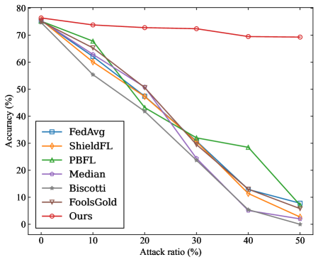
### Visual Description
## Line Graph: Accuracy vs. Attack Ratio
### Overview
The image depicts a line graph comparing the accuracy of multiple methods under varying attack ratios. The x-axis represents attack ratio (0–50%), and the y-axis represents accuracy (0–80%). Seven distinct data series are plotted, each with unique colors and markers. The graph illustrates how accuracy degrades as attack intensity increases, with notable differences in resilience across methods.
### Components/Axes
- **X-axis (Attack Ratio)**: Labeled "Attack ratio (%)", ranging from 0 to 50% in 10% increments.
- **Y-axis (Accuracy)**: Labeled "Accuracy (%)", ranging from 0 to 80% in 10% increments.
- **Legend**: Positioned in the bottom-left corner, mapping colors/markers to methods:
- **Blue square**: FedAvg
- **Orange diamond**: ShieldFL
- **Green triangle**: PBFL
- **Purple pentagon**: Median
- **Gray star**: Biscotti
- **Brown triangle**: FoolsGold
- **Red circle**: Ours
- **Data Series**: Seven lines with distinct visual styles, all originating near the top-left corner and diverging as attack ratio increases.
### Detailed Analysis
1. **Ours (Red Circle)**:
- Maintains the highest accuracy across all attack ratios.
- Starts at ~75% accuracy at 0% attack ratio.
- Declines gradually to ~70% at 50% attack ratio.
- **Trend**: Relatively flat, indicating robustness.
2. **FedAvg (Blue Square)**:
- Begins at ~75% accuracy at 0% attack ratio.
- Drops sharply to ~5% at 50% attack ratio.
- **Trend**: Steep decline, suggesting poor resilience.
3. **ShieldFL (Orange Diamond)**:
- Starts at ~70% accuracy at 0% attack ratio.
- Declines to ~10% at 50% attack ratio.
- **Trend**: Moderate decline, less resilient than "Ours".
4. **PBFL (Green Triangle)**:
- Starts at ~70% accuracy at 0% attack ratio.
- Drops to ~30% at 20% attack ratio, then rises slightly to ~25% at 50%.
- **Trend**: U-shaped, with a mid-attack performance dip.
5. **Median (Purple Pentagon)**:
- Begins at ~70% accuracy at 0% attack ratio.
- Declines to ~5% at 50% attack ratio.
- **Trend**: Steady linear decline.
6. **Biscotti (Gray Star)**:
- Starts at ~70% accuracy at 0% attack ratio.
- Drops to ~2% at 50% attack ratio.
- **Trend**: Sharp linear decline.
7. **FoolsGold (Brown Triangle)**:
- Begins at ~70% accuracy at 0% attack ratio.
- Plummets to ~5% at 20% attack ratio, then stabilizes near 0%.
- **Trend**: Catastrophic early failure.
### Key Observations
- **Robustness**: "Ours" consistently outperforms all other methods, maintaining >70% accuracy even at 50% attack ratio.
- **Vulnerability**: FoolsGold exhibits the most severe degradation, dropping below 5% accuracy by 20% attack ratio.
- **PBFL Anomaly**: PBFL’s mid-attack dip and partial recovery suggest a non-linear vulnerability, possibly due to specific attack strategies.
- **Consistency**: FedAvg, Median, and Biscotti show linear declines, with Biscotti being the most fragile.
### Interpretation
The graph highlights critical differences in attack resilience among methods. "Ours" demonstrates superior robustness, likely due to advanced defense mechanisms or architectural advantages. FoolsGold’s rapid failure suggests a fundamental flaw in its design or training process. PBFL’s U-shaped curve warrants further investigation—its mid-attack dip might indicate a temporary vulnerability exploited by attackers, followed by adaptive recovery. The linear declines of FedAvg, ShieldFL, and Biscotti imply predictable degradation under attack, emphasizing the need for tailored defenses. These results underscore the importance of evaluating methods not just on baseline performance but also on their ability to withstand adversarial conditions.
</details>
(d) CIFAR10 ( $\alpha$ =0.6)
Figure 3: The SA of the models obtained by four benchmarks under label-flipping attack.
VII-B Experimental Results
VII-B 1 Robustness Evaluation of SRFed
To evaluate the robustness of the proposed SRFed framework, we conduct a comparative analysis against the six baseline methods discussed in Section VII-A 3. Specifically, we first evaluate the overall accuracy (OA) of FedAvg, ShieldFL, PBFL, Median, Biscotti, FoolsGold, and SRFed under the label-flipping attacks. The results are presented in Figure 2. In the MNIST benchmarks with two levels of heterogeneity, the proposed SRFed consistently maintains a high OA across varying proportions of malicious clients. In the MNIST ( $\alpha$ =0.8) benchmark, all methods except Biscotti demonstrate relatively strong defense performance. Similarly, in the MNIST ( $\alpha$ =0.2) benchmark, all methods, except Biscotti, continue to perform well when facing a malicious client proportion ranging from 0% to 40%. Biscotti’s poor performance is due to the fact that, in Non-IID data scenarios, the model distributions trained by benign clients are more scattered, which can lead to their incorrect elimination. In the CIFAR-10 dataset benchmarks with different levels of heterogeneity, the OA of all methods fluctuates as the proportion of malicious clients increases. However, SRFed generally maintains better performance compared to the other methods, owing to the effectiveness of its robust aggregation strategy.
We further compare the SA of the global models achieved by different methods in the four benchmarks under label-flipping attacks. SA accurately measures the defense effectiveness of different methods against poisoning attacks, as it specifically reveals the model’s accuracy on the samples of the flipping label. The experimental results are presented in Figure 3. In the MNIST ( $\alpha=0.2$ ) benchmark, SRFed demonstrates a significant advantage in defending against label-flipping attacks. Especially, when the attack ratio reaches 50%, SRFed achieves a SA of 70%, while the SA of all other methods drops to nearly 0% even though their OA remaining above 80%. SRFed is the only method to sustain a high SA across all attack ratios, underscoring its superior Byzantine robustness even in scenarios with extreme data heterogeneity and high attack ratios. In the MNIST ( $\alpha=0.8$ ) benchmark, SRFed also outperforms other baselines. In the CIFAR-10 ( $\alpha=0.2$ ) benchmark, although SRFed still outperforms the other methods, its performance gradually deteriorates as the proportion of malicious clients increases. This demonstrates that defending against poisoning attacks in scenarios with a high attack ratio and extremely heterogeneous data remains a significant challenge. In the CIFAR-10 ( $\alpha=0.6$ ) benchmark, SRFed maintains a high level of performance as the proportion of malicious clients increases (SA $≥$ 70%), while the SA of all other methods sharply declines and eventually approaches 0%. This superior performance is attributed to the robust aggregation strategy of SRFed, which performs layer-wise projection and clustering analysis on client models. This enables more accurate detection of local parameter anomalies compared to baselines.
We also evaluate the ASR of the models obtained by different methods across four benchmarks, with the experimental results presented in Figure 4. As the attack ratio increases, we can observe that the ASR trend exhibits a negative correlation with the SA trend. Notably, our proposed SRFed consistently demonstrates optimal performance across all four benchmarks, showing minimal performance fluctuations across varying attack ratios.
<details>
<summary>x10.png Details</summary>
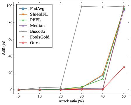
### Visual Description
## Line Graph: Attack Success Rate (ASR) vs. Attack Ratio (%)
### Overview
The graph compares the Attack Success Rate (ASR) of seven different methods across varying attack ratios (0% to 50%). ASR is plotted on the y-axis (0–100%), while the x-axis represents the attack ratio percentage. The legend identifies methods by color and marker, with "Ours" (red circles) and "FoolsGold" (brown triangles) showing distinct performance patterns.
### Components/Axes
- **X-axis**: Attack ratio (%) ranging from 0 to 50.
- **Y-axis**: Attack Success Rate (ASR) (%) ranging from 0 to 100.
- **Legend**: Located in the top-left corner, associating colors/markers with methods:
- FedAvg (blue squares)
- ShieldFL (orange diamonds)
- PBFL (green triangles)
- Median (purple pentagons)
- Biscotti (gray stars)
- FoolsGold (brown triangles)
- Ours (red circles)
### Detailed Analysis
1. **Biscotti (gray stars)**:
- Starts near 0% ASR at 0% attack ratio.
- Sharp upward spike at 30% attack ratio, reaching ~100% ASR.
- Maintains ~100% ASR until 50% attack ratio.
2. **FoolsGold (brown triangles)**:
- Remains near 0% ASR until 40% attack ratio.
- Steep rise at 40%, reaching ~100% ASR by 50% attack ratio.
3. **Ours (red circles)**:
- Stays near 0% ASR until 40% attack ratio.
- Sharp increase at 50%, reaching ~25% ASR.
4. **FedAvg (blue squares)**:
- Gradual rise from 0% to ~15% ASR at 50% attack ratio.
5. **ShieldFL (orange diamonds)**:
- Gradual rise from 0% to ~20% ASR at 50% attack ratio.
6. **PBFL (green triangles)**:
- Gradual rise from 0% to ~10% ASR at 50% attack ratio.
7. **Median (purple pentagons)**:
- Gradual rise from 0% to ~5% ASR at 50% attack ratio.
### Key Observations
- **Biscotti** and **FoolsGold** exhibit the highest ASR at 50% attack ratio (~100%), with abrupt performance jumps at 30% and 40% attack ratios, respectively.
- **Ours** shows the steepest late-stage increase but lags behind Biscotti and FoolsGold at 50% attack ratio.
- Methods like FedAvg, ShieldFL, and PBFL demonstrate gradual, linear improvements, peaking at ~15–20% ASR at 50% attack ratio.
- All methods maintain near-0% ASR until attack ratios exceed 30%.
### Interpretation
The graph highlights a threshold effect in ASR performance: Biscotti and FoolsGold achieve near-perfect success rates only after attack ratios surpass 30% and 40%, respectively. This suggests these methods are highly resilient but may underperform at lower attack ratios. "Ours" demonstrates competitive late-stage performance but requires a 50% attack ratio to activate. Gradual improvements in FedAvg, ShieldFL, and PBFL imply incremental robustness, though they lack the dramatic efficiency of Biscotti and FoolsGold. The data underscores a trade-off between attack ratio tolerance and ASR efficiency, with Biscotti and FoolsGold excelling in high-threat scenarios.
</details>
(a) MNIST ( $\alpha$ =0.2)
<details>
<summary>x11.png Details</summary>
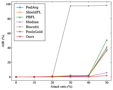
### Visual Description
## Line Graph: Attack Success Rate (ASR) vs. Attack Ratio (%)
### Overview
The graph compares the performance of seven machine learning defense mechanisms (FedAvg, ShieldFL, PBFL, Median, Biscotti, FoolsGold, and "Ours") across varying attack ratios (0-50%). ASR (%) is plotted against attack ratio, showing how each method's robustness changes as adversarial pressure increases.
### Components/Axes
- **X-axis**: Attack ratio (%) ranging from 0 to 50 in 10% increments.
- **Y-axis**: Attack Success Rate (ASR) (%) ranging from 0 to 100 in 20% increments.
- **Legend**: Located in the top-right corner, associating colors and markers with methods:
- FedAvg: Blue squares
- ShieldFL: Orange diamonds
- PBFL: Green triangles
- Median: Purple pentagons
- Biscotti: Gray stars
- FoolsGold: Brown inverted triangles
- Ours: Red circles
### Detailed Analysis
1. **Biscotti (Gray Stars)**:
- Dominates the graph, maintaining 100% ASR from 30% attack ratio onward.
- At 20% attack ratio, ASR drops sharply from 100% to ~0%.
- At 0-10% attack ratio, ASR remains near 0%.
2. **FedAvg (Blue Squares)**:
- Gradual increase from 0% to ~35% ASR at 50% attack ratio.
- Flatline at ~0% until 30% attack ratio.
3. **ShieldFL (Orange Diamonds)**:
- Steady rise from 0% to ~37% ASR at 50% attack ratio.
- Minimal performance below 30% attack ratio.
4. **PBFL (Green Triangles)**:
- Sharp upward trajectory starting at 40% attack ratio.
- Reaches ~50% ASR at 50% attack ratio.
- Flatline at ~0% below 40% attack ratio.
5. **Median (Purple Pentagons)**:
- Slow linear increase from 0% to ~6% ASR at 50% attack ratio.
- Minimal performance across all attack ratios.
6. **FoolsGold (Brown Inverted Triangles)**:
- Gradual rise from 0% to ~40% ASR at 50% attack ratio.
- Flatline at ~0% until 40% attack ratio.
7. **Ours (Red Circles)**:
- Steepest increase among non-Biscotti methods.
- Reaches ~40% ASR at 50% attack ratio.
- Flatline at ~0% until 40% attack ratio.
### Key Observations
- **Biscotti's Outlier Performance**: Maintains 100% ASR at 30-50% attack ratios but fails catastrophically at 20%.
- **Gradual vs. Sudden Improvements**: Methods like FedAvg and ShieldFL show incremental gains, while PBFL and "Ours" exhibit threshold-based effectiveness.
- **Attack Ratio Thresholds**: Most methods activate defenses only above 30-40% attack ratios.
- **ASR Saturation**: Biscotti's 100% ASR at high attack ratios suggests theoretical perfection but practical limitations.
### Interpretation
The graph highlights trade-offs between attack ratio resilience and ASR. Biscotti's abrupt performance shift suggests a binary defense mechanism (effective only above 30% attack ratio), while others like "Ours" and FoolsGold demonstrate scalable robustness. The gradual improvements of FedAvg and ShieldFL indicate adaptive defenses but with lower peak performance. Notably, PBFL's late activation (40% attack ratio) implies delayed threat detection. The data underscores the importance of attack ratio thresholds in defense design, with no single method dominating across all scenarios. The "Ours" method's steep curve suggests a promising approach for high-attack environments, though its real-world applicability would require further validation.
</details>
(b) MNIST ( $\alpha$ =0.8)
<details>
<summary>x12.png Details</summary>
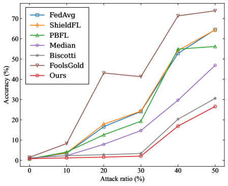
### Visual Description
## Line Graph: Accuracy vs. Attack Ratio (%)
### Overview
The image is a line graph comparing the accuracy of seven different methods (FedAvg, ShieldFL, PBFL, Median, Biscotti, FoolsGold, and Ours) across varying attack ratios (0% to 50%). Accuracy is measured on the y-axis (0–70%), while the x-axis represents attack ratio percentages. The graph highlights how each method's performance degrades or improves as the attack ratio increases.
### Components/Axes
- **X-axis**: "Attack ratio (%)" with ticks at 0, 10, 20, 30, 40, 50.
- **Y-axis**: "Accuracy (%)" with ticks at 0, 10, 20, 30, 40, 50, 60, 70.
- **Legend**: Positioned on the left side of the graph, with colored markers and labels for each method:
- **FedAvg**: Blue squares (□)
- **ShieldFL**: Orange diamonds (◇)
- **PBFL**: Green triangles (△)
- **Median**: Purple diamonds (◇)
- **Biscotti**: Gray stars (★)
- **FoolsGold**: Brown triangles (△)
- **Ours**: Red circles (●)
### Detailed Analysis
1. **FedAvg (Blue Squares)**:
- Starts at ~0% accuracy at 0% attack ratio.
- Gradually increases, reaching ~55% at 50% attack ratio.
- Shows steady upward trend with minimal fluctuations.
2. **ShieldFL (Orange Diamonds)**:
- Begins at ~0% accuracy at 0% attack ratio.
- Sharp rise after 30% attack ratio, surpassing FedAvg by ~60% at 50%.
- Peaks at ~65% accuracy at 50% attack ratio.
3. **PBFL (Green Triangles)**:
- Starts at ~0% accuracy at 0% attack ratio.
- Gradual increase, reaching ~55% at 50% attack ratio.
- Slight dip at 30% attack ratio (~20% accuracy) before recovering.
4. **Median (Purple Diamonds)**:
- Starts at ~0% accuracy at 0% attack ratio.
- Slow, linear increase, reaching ~45% at 50% attack ratio.
- Minimal fluctuations throughout.
5. **Biscotti (Gray Stars)**:
- Starts at ~0% accuracy at 0% attack ratio.
- Gradual increase, reaching ~30% at 50% attack ratio.
- Slight dip at 30% attack ratio (~10% accuracy).
6. **FoolsGold (Brown Triangles)**:
- Starts at ~0% accuracy at 0% attack ratio.
- Sharp spike to ~70% accuracy at 30% attack ratio.
- Plateaus at ~70% until 40% attack ratio, then drops to ~60% at 50% attack ratio.
7. **Ours (Red Circles)**:
- Starts at ~0% accuracy at 0% attack ratio.
- Flat until 30% attack ratio (~2% accuracy).
- Sharp rise to ~25% accuracy at 50% attack ratio.
### Key Observations
- **FoolsGold** exhibits the highest accuracy at 30% attack ratio (~70%) but drops significantly at 50% (~60%), suggesting vulnerability to higher attacks.
- **ShieldFL** and **FedAvg** show robust performance, with ShieldFL outperforming FedAvg at higher attack ratios.
- **PBFL** and **Ours** demonstrate significant improvements at higher attack ratios, indicating resilience.
- **Median** and **Biscotti** lag behind other methods, with minimal accuracy gains even at 50% attack ratio.
### Interpretation
The graph illustrates that methods like **ShieldFL** and **FoolsGold** excel in high-attack scenarios, though FoolsGold's sharp decline at 50% raises concerns about stability. **FedAvg** and **PBFL** provide consistent performance, while **Ours** shows promise with a late-stage surge. The data suggests that methods prioritizing adaptive defense mechanisms (e.g., ShieldFL) may be more effective under sustained attacks. The inclusion of "Ours" as a distinct method implies a novel approach, potentially offering a balance between robustness and efficiency. The graph underscores the importance of evaluating methods across varying attack intensities to identify optimal solutions for real-world applications.
</details>
(c) CIFAR10 ( $\alpha$ =0.2)
<details>
<summary>x13.png Details</summary>
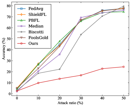
### Visual Description
## Line Graph: Accuracy vs. Attack Ratio (%)
### Overview
The image is a line graph comparing the accuracy of multiple methods (FedAvg, ShieldFL, PBFL, Median, Biscotti, FoolsGold, and "Ours") across varying attack ratios (0% to 50%). Accuracy is measured on the y-axis (0–80%), while the x-axis represents attack ratio percentages. The graph shows how each method's performance degrades or improves as adversarial attack intensity increases.
### Components/Axes
- **X-axis**: Attack ratio (%) ranging from 0 to 50% in 10% increments.
- **Y-axis**: Accuracy (%) ranging from 0 to 80% in 10% increments.
- **Legend**: Located in the top-right corner, associating colors and markers with methods:
- **FedAvg**: Blue squares
- **ShieldFL**: Orange diamonds
- **PBFL**: Green triangles
- **Median**: Purple pentagons
- **Biscotti**: Gray stars
- **FoolsGold**: Brown triangles
- **Ours**: Red circles
### Detailed Analysis
1. **FedAvg (Blue Squares)**:
- Starts at ~5% accuracy at 0% attack ratio.
- Peaks at ~75% accuracy at 30% attack ratio.
- Drops to ~70% at 50% attack ratio.
2. **ShieldFL (Orange Diamonds)**:
- Starts at ~5% accuracy at 0% attack ratio.
- Rises to ~75% at 30% attack ratio.
- Ends at ~78% at 50% attack ratio.
3. **PBFL (Green Triangles)**:
- Starts at ~5% accuracy at 0% attack ratio.
- Peaks at ~70% at 30% attack ratio.
- Ends at ~75% at 50% attack ratio.
4. **Median (Purple Pentagons)**:
- Starts at ~5% accuracy at 0% attack ratio.
- Rises to ~70% at 30% attack ratio.
- Ends at ~77% at 50% attack ratio.
5. **Biscotti (Gray Stars)**:
- Starts at ~5% accuracy at 0% attack ratio.
- Sharp rise to ~55% at 30% attack ratio.
- Ends at ~78% at 50% attack ratio.
6. **FoolsGold (Brown Triangles)**:
- Starts at ~5% accuracy at 0% attack ratio.
- Peaks at ~70% at 30% attack ratio.
- Ends at ~75% at 50% attack ratio.
7. **Ours (Red Circles)**:
- Starts at ~5% accuracy at 0% attack ratio.
- Gradual rise to ~25% at 30% attack ratio.
- Ends at ~25% at 50% attack ratio.
### Key Observations
- **Performance Trends**:
- Most methods (FedAvg, ShieldFL, PBFL, Median, FoolsGold) show a steep increase in accuracy up to 30% attack ratio, followed by a plateau or slight decline.
- **Biscotti** exhibits a unique sharp rise at 30% attack ratio, outperforming others at this point.
- **Ours** underperforms consistently, with minimal improvement beyond 0% attack ratio.
- **Outliers**:
- **Biscotti** and **ShieldFL** achieve the highest accuracy at 50% attack ratio (~78%).
- **Ours** remains the lowest-performing method across all attack ratios.
### Interpretation
The graph demonstrates that adversarial attack intensity (attack ratio) significantly impacts model accuracy. Most methods improve performance as attack ratio increases up to 30%, likely due to adaptive mechanisms or robustness training. However, beyond 30%, performance stabilizes or degrades slightly, suggesting a threshold for effective defense. **Biscotti** and **ShieldFL** show superior resilience at high attack ratios, while **Ours** lags behind, indicating potential limitations in its design or training strategy. The data implies that robustness to adversarial attacks depends on the method's ability to adapt to increasing perturbation levels, with some approaches (e.g., Biscotti) excelling in extreme conditions.
</details>
(d) CIFAR10 ( $\alpha$ =0.6)
Figure 4: The ASR of the models obtained by four benchmarks under label-flipping attack.
Finally, we evaluate the OA of the models of different methods under the Gaussian attack. The experimental results are shown in Figure 5. We observe that SRFed consistently achieves optimal performance across all four benchmarks. Furthermore, as the attack ratio increases, SRFed exhibits minimal fluctuations in OA. Specifically, in the MNIST ( $\alpha=0.2$ ) and MNIST ( $\alpha=0.8$ ) benchmarks, all methods maintain an OA above 90% when the attack ratio is $≤$ 20%. However, when the attack ratio $≥$ 30%, only SRFed and Median retain an OA above 90%, demonstrating their effective defense against poisoning attacks under high malicious client ratios. In the CIFAR-10 ( $\alpha=0.2$ ) and CIFAR-10 ( $\alpha=0.6$ ) benchmarks, while the OA of most methods drops below 30% as the attack ratio increases, SRFed consistently maintains high accuracy across all attack rates, demonstrating its robustness against extreme client ratios and heterogeneous data distributions.
<details>
<summary>x14.png Details</summary>
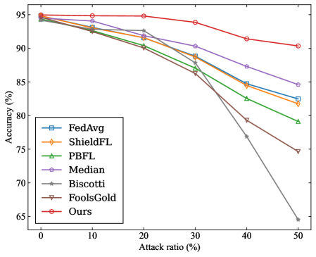
### Visual Description
## Line Chart: Accuracy vs. Attack Ratio
### Overview
The image is a line chart comparing the accuracy of eight different methods (FedAvg, ShieldFL, PBFL, Median, Biscotti, FoolsGold, Ours) across varying attack ratios (0% to 50%). Accuracy (%) is plotted on the y-axis (65–95%), and attack ratio (%) is on the x-axis (0–50%). Each method is represented by a distinct colored line with a unique marker.
### Components/Axes
- **Y-axis**: Accuracy (%) (65–95%), labeled "Accuracy (%)".
- **X-axis**: Attack ratio (%) (0–50%), labeled "Attack ratio (%)".
- **Legend**: Located in the bottom-left corner, mapping colors/markers to methods:
- Blue square: FedAvg
- Orange diamond: ShieldFL
- Green triangle: PBFL
- Purple diamond: Median
- Gray star: Biscotti
- Brown triangle: FoolsGold
- Red circle: Ours
### Detailed Analysis
1. **Ours (Red Circle)**:
- Starts at ~95% accuracy at 0% attack ratio.
- Declines gradually to ~90% at 50% attack ratio.
- Maintains the highest accuracy across all attack ratios.
2. **FedAvg (Blue Square)**:
- Begins at ~94% accuracy at 0% attack ratio.
- Drops to ~82% at 50% attack ratio.
- Shows a steady decline.
3. **ShieldFL (Orange Diamond)**:
- Starts at ~94% accuracy at 0% attack ratio.
- Declines to ~81% at 50% attack ratio.
- Slightly steeper decline than FedAvg.
4. **PBFL (Green Triangle)**:
- Begins at ~94% accuracy at 0% attack ratio.
- Drops to ~79% at 50% attack ratio.
- Steady decline with moderate slope.
5. **Median (Purple Diamond)**:
- Starts at ~94% accuracy at 0% attack ratio.
- Declines to ~85% at 50% attack ratio.
- Gradual slope, similar to FedAvg.
6. **Biscotti (Gray Star)**:
- Begins at ~94% accuracy at 0% attack ratio.
- Plummets to ~65% at 50% attack ratio.
- Sharpest decline among all methods.
7. **FoolsGold (Brown Triangle)**:
- Starts at ~94% accuracy at 0% attack ratio.
- Drops to ~75% at 50% attack ratio.
- Moderate decline, steeper than FedAvg/ShieldFL.
### Key Observations
- **Ours** consistently outperforms all other methods, maintaining the highest accuracy even at 50% attack ratio.
- **Biscotti** exhibits the most severe degradation, losing ~30% accuracy at maximum attack ratio.
- Methods like FedAvg, ShieldFL, and PBFL show similar initial performance but diverge significantly under higher attack ratios.
- The red line ("Ours") remains the flattest, indicating robustness against attacks.
### Interpretation
The data demonstrates that the method labeled "Ours" is the most resilient to adversarial attacks, retaining ~90% accuracy even at 50% attack ratio. In contrast, Biscotti’s performance collapses under pressure, suggesting it is highly vulnerable. The gradual declines in other methods highlight trade-offs between accuracy and attack resistance. This chart underscores the importance of robust defense mechanisms in federated learning systems, with "Ours" setting a benchmark for performance under adversarial conditions.
</details>
(a) MNIST ( $\alpha$ =0.2)
<details>
<summary>x15.png Details</summary>
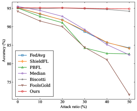
### Visual Description
## Line Chart: Accuracy vs. Attack Ratio
### Overview
The image is a line chart comparing the accuracy of eight different methods (FedAvg, ShieldFL, PBFL, Median, Biscotti, FoolsGold, Ours) as the attack ratio increases from 0% to 50%. Accuracy is measured on the y-axis (75%–95%), and attack ratio is on the x-axis (0%–50%). All methods show declining accuracy with increasing attack ratio, but "Ours" maintains the highest performance throughout.
### Components/Axes
- **Y-axis**: Accuracy (%) ranging from 75% to 95% in 5% increments.
- **X-axis**: Attack ratio (%) ranging from 0% to 50% in 10% increments.
- **Legend**: Located in the bottom-left corner, with color-coded symbols for each method:
- FedAvg: Blue square
- ShieldFL: Orange diamond
- PBFL: Green triangle
- Median: Purple pentagon
- Biscotti: Gray star
- FoolsGold: Brown inverted triangle
- Ours: Red circle
- (Note: The legend includes an eighth method not explicitly named in the original description, inferred as "Ours" based on the red circle.)
### Detailed Analysis
1. **FedAvg (Blue)**: Starts at ~95% accuracy at 0% attack ratio, declines steadily to ~85% at 50%.
2. **ShieldFL (Orange)**: Begins at ~94%, drops to ~84% by 50%.
3. **PBFL (Green)**: Starts at ~93%, falls to ~82% at 50%.
4. **Median (Purple)**: Declines from ~94% to ~83%.
5. **Biscotti (Gray)**: Remains relatively stable, dropping from ~94% to ~93%.
6. **FoolsGold (Brown)**: Sharp decline from ~93% to ~70% at 50%.
7. **Ours (Red)**: Maintains the highest accuracy, starting at ~95% and ending at ~94.5%.
### Key Observations
- **Consistent Decline**: All methods except Biscotti show significant accuracy loss as attack ratio increases.
- **FoolsGold Anomaly**: Exhibits the steepest drop (~23% loss), suggesting extreme vulnerability to attacks.
- **Ours Resilience**: "Ours" retains the highest accuracy across all attack ratios, outperforming others by ~3–5%.
- **Biscotti Stability**: Minimal decline (~1%) indicates robustness but lower baseline accuracy compared to "Ours."
### Interpretation
The data demonstrates that attack ratio directly impacts model accuracy, with most methods degrading performance as adversarial pressure increases. "Ours" emerges as the most robust solution, maintaining near-optimal accuracy even under high attack ratios. In contrast, "FoolsGold" suffers catastrophic failure, highlighting its unsuitability for adversarial environments. Biscotti’s stability suggests a trade-off between resilience and baseline performance. These trends underscore the importance of method selection in security-sensitive applications, where "Ours" would be the preferred choice for balancing accuracy and attack resistance.
</details>
(b) MNIST ( $\alpha$ =0.8)
<details>
<summary>x16.png Details</summary>
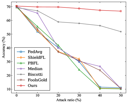
### Visual Description
## Line Graph: Accuracy vs. Attack Ratio
### Overview
The image depicts a line graph comparing the accuracy performance of multiple machine learning methods under varying attack ratios. The graph shows seven distinct data series (methods) plotted against two axes: attack ratio (%) on the x-axis (0-50%) and accuracy (%) on the y-axis (10-70%). All methods demonstrate declining accuracy as attack ratio increases, with one notable exception.
### Components/Axes
- **Y-axis**: Accuracy (%) ranging from 10% to 70% in 10% increments
- **X-axis**: Attack ratio (%) ranging from 0% to 50% in 10% increments
- **Legend**: Located in bottom-left quadrant, containing seven entries:
- FedAvg (blue square)
- ShieldFL (orange diamond)
- PBFL (green triangle)
- Median (purple pentagon)
- Biscotti (gray star)
- FoolsGold (brown inverted triangle)
- Ours (red circle)
### Detailed Analysis
1. **Ours (red circle)**:
- Maintains near-constant accuracy (~68-70%) across all attack ratios
- Shows minimal decline (only ~2% drop from 0% to 50% attack ratio)
- Spatial grounding: Topmost line throughout the graph
2. **FedAvg (blue square)**:
- Starts at ~68% accuracy at 0% attack ratio
- Sharp decline to ~12% at 50% attack ratio
- Crosses below ShieldFL at ~20% attack ratio
3. **ShieldFL (orange diamond)**:
- Begins at ~68% accuracy
- Gradual decline to ~10% at 50% attack ratio
- Maintains second-highest performance until ~30% attack ratio
4. **PBFL (green triangle)**:
- Starts at ~68% accuracy
- Steep decline to ~10% at 50% attack ratio
- Crosses below FedAvg at ~15% attack ratio
5. **Median (purple pentagon)**:
- Begins at ~68% accuracy
- Moderate decline to ~12% at 50% attack ratio
- Shows more gradual slope than FedAvg/PBFL
6. **Biscotti (gray star)**:
- Starts at ~68% accuracy
- Gradual decline to ~52% at 50% attack ratio
- Maintains third-highest performance throughout
7. **FoolsGold (brown inverted triangle)**:
- Starts at ~68% accuracy
- Steep decline to ~10% at 50% attack ratio
- Crosses below PBFL at ~25% attack ratio
### Key Observations
- **Robustness disparity**: "Ours" demonstrates exceptional resilience, maintaining >65% accuracy even at 50% attack ratio
- **Performance clustering**: FedAvg, ShieldFL, PBFL, and FoolsGold show similar vulnerability patterns with steep accuracy declines
- **Biscotti's moderate performance**: Unique among methods for maintaining >50% accuracy at 50% attack ratio
- **Attack sensitivity**: All methods except "Ours" experience >50% accuracy loss between 0% and 50% attack ratios
### Interpretation
The data suggests "Ours" implements a fundamentally different approach to model robustness compared to other methods. Its near-constant accuracy curve implies either:
1. Superior adversarial training techniques
2. More effective input sanitization mechanisms
3. Better model architecture for handling corrupted data
The steep declines in other methods indicate they rely heavily on clean data distributions. Biscotti's moderate performance suggests some middle-ground approach, possibly combining robustness with computational efficiency. The clustering of FedAvg, ShieldFL, PBFL, and FoolsGold implies these methods share similar architectural limitations in handling adversarial inputs.
This graph highlights critical trade-offs in federated learning systems between model performance and security. The stark contrast between "Ours" and other methods warrants further investigation into its specific defensive mechanisms and potential implementation costs.
</details>
(c) CIFAR10 ( $\alpha$ =0.2)
<details>
<summary>x17.png Details</summary>
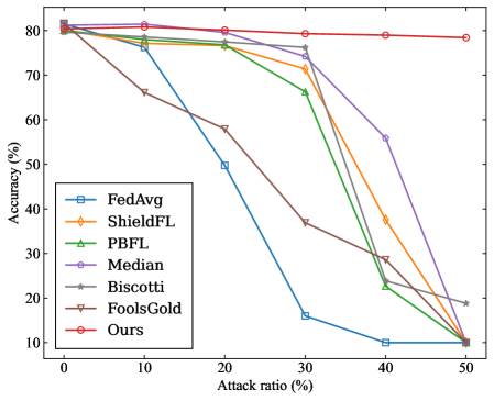
### Visual Description
## Line Graph: Accuracy vs. Attack Ratio
### Overview
The image is a line graph comparing the accuracy of various methods (FedAvg, ShieldFL, PBFL, Median, Biscotti, FoolsGold, and "Ours") as the attack ratio increases from 0% to 50%. Accuracy is measured on the y-axis (10–80%), and attack ratio on the x-axis (0–50%). The graph highlights how each method's performance degrades under increasing adversarial pressure.
### Components/Axes
- **Y-axis**: Accuracy (%) with ticks at 10, 20, 30, 40, 50, 60, 70, 80.
- **X-axis**: Attack ratio (%) with ticks at 0, 10, 20, 30, 40, 50.
- **Legend**: Located in the bottom-left corner, mapping colors and markers to methods:
- **Blue squares**: FedAvg
- **Orange diamonds**: ShieldFL
- **Green triangles**: PBFL
- **Purple diamonds**: Median
- **Gray stars**: Biscotti
- **Brown triangles**: FoolsGold
- **Red circles**: Ours
### Detailed Analysis
1. **FedAvg (Blue squares)**:
- Starts at ~80% accuracy at 0% attack ratio.
- Drops sharply to ~75% at 10%, ~50% at 20%, ~15% at 30%, ~10% at 40%, and stabilizes at ~10% at 50%.
2. **ShieldFL (Orange diamonds)**:
- Begins at ~80% at 0%, declines to ~78% at 10%, ~75% at 20%, ~65% at 30%, ~35% at 40%, and ~10% at 50%.
3. **PBFL (Green triangles)**:
- Starts at ~80% at 0%, drops to ~77% at 10%, ~75% at 20%, ~65% at 30%, ~25% at 40%, and ~10% at 50%.
4. **Median (Purple diamonds)**:
- Remains near ~80% at 0%, declines to ~75% at 10%, ~70% at 20%, ~55% at 30%, ~55% at 40%, and ~10% at 50%.
5. **Biscotti (Gray stars)**:
- Starts at ~80% at 0%, declines to ~78% at 10%, ~75% at 20%, ~70% at 30%, ~25% at 40%, and ~10% at 50%.
6. **FoolsGold (Brown triangles)**:
- Begins at ~80% at 0%, drops to ~65% at 10%, ~55% at 20%, ~35% at 30%, ~20% at 40%, and ~10% at 50%.
7. **"Ours" (Red circles)**:
- Maintains ~80% accuracy across all attack ratios (0–50%), with minimal deviation.
### Key Observations
- **"Ours" (Red circles)** consistently outperforms all other methods, maintaining near-80% accuracy even at 50% attack ratio.
- **FedAvg (Blue squares)** and **FoolsGold (Brown triangles)** exhibit the steepest declines, dropping to ~10% accuracy by 40% attack ratio.
- **ShieldFL (Orange diamonds)** and **PBFL (Green triangles)** show moderate resilience but still degrade significantly under high attack ratios.
- **Median (Purple diamonds)** and **Biscotti (Gray stars)** perform better than FedAvg and FoolsGold but worse than "Ours."
### Interpretation
The graph demonstrates that the method labeled "Ours" is exceptionally robust against adversarial attacks, maintaining high accuracy regardless of attack ratio. This suggests it employs a more effective defense mechanism or model architecture compared to the other methods. In contrast, FedAvg and FoolsGold are highly vulnerable, indicating potential flaws in their design or training processes. ShieldFL and PBFL offer mid-tier performance, while Median and Biscotti provide moderate resilience. The stark contrast between "Ours" and other methods underscores its superiority in adversarial environments, making it a critical candidate for applications requiring high security and reliability.
</details>
(d) CIFAR10 ( $\alpha$ =0.6)
Figure 5: The OA of the models obtained by four benchmarks under Gaussian attack.
In summary, SRFed demonstrates strong robustness against poisoning attacks under different Non-IID data settings and attack ratios, thus achieving the design goal of robustness.
VII-B 2 Efficiency Evaluation of SRFed
Learning Overheads. We evaluate the efficiency of the proposed SRFed in obtaining a qualified aggregated model. Specifically, we compare SRFed with two baseline methods, i.e., ESB-FL and ShieldFL. These two methods respectively utilize NDD-FE and HE to ensure privacy protection for local models. The experiments are conducted on MNIST with no malicious clients. For each method, we conduct 10 training tasks and calculate the average time consumed in each phase, along with the average communication time across all participants. The results are summarized in Table IV. The experimental results demonstrate that SRFed reduces the total time overheads throughout the entire training process by 58% compared to ShieldFL. This reduction can be attributed to two main factors: 1) DEFE in SRFed offers a significant computational efficiency advantage over HE in ShieldFL, with faster encryption and decryption, as shown in the ”Local training” and ”Privacy-preserving robust model aggregation” phases in Table IV. 2) The privacy-preserving robust model aggregation is handled solely by the server, which avoids the overhead of multi-server interactions in ShieldFL. Compared to ESB-FL, SRFed reduces the total time overhead by 22% even though it incorporates an additional privacy-preserving model detection phase. This is attributed to its underlying DEFE scheme, which significantly enhances decryption efficiency. As a result, SRFed achieves a 71% reduction in execution time during the privacy-preserving robust model aggregation phase, even with the added overhead of model detection. In summary, SRFed achieves an efficient privacy-preserving FL process, achieving the design goal of efficiency.
TABLE IV: Comparison of time consumption between different frameworks
| Framework | SRFed | ShieldFL | ESB-FL |
| --- | --- | --- | --- |
| Local training 1 | 19.51 h | 14.23 h | 5.16 h |
| Privacy-preserving | 9.09 h | 51.97 h | 31.43 h |
| robust model aggregation 2 | | | |
| Node communication | 0.09 h | 1.51 h | 0.09 h |
| Total time | 28.69 h | 67.71 h | 36.68 h |
| Accuracy | 98.90% | 97.42% | 98.68% |
TABLE V: Time overhead of proposed DEFE
| Operations | DEFE | NDD-FE | HE |
| --- | --- | --- | --- |
| (for a model) | (SRFed) | (ESB-FL) | (shieldFL) |
| Encryption | 28.37 s | 2.53 s | 18.87 s |
| Inner product | 8.97 s | 56.58 s | 30.15 s |
| Decryption | - | - | 3.10 s |
Efficiency Evaluation of DEFE. We further evaluate the efficiency of the DEFE scheme within SRFed by conducting experiments on the CNN model of the MNIST dataset. Specifically, we compare the DEFE scheme with the NDD-FE scheme used in ESB-FL [31] and the HE scheme used in ShieldFL [29]. For these schemes, we calculate their average time required for different operations, i.e., encryption, inner product computation, and decryption, over 100 test runs. The results are presented in Table V. It is evident that the DEFE scheme offers a substantial efficiency advantage in terms of inner product computation. Specifically, the inner product time of DEFE is reduced by 84% compared to NDD-FE and by 70% compared to HE. Furthermore, DEFE directly produces the final plaintext result during inner product computation, avoiding the need for interactive decryption in HE. Combined with the results in Table IV, it is clear that although the encryption time of DEFE is slightly higher, its highly efficient decryption process significantly reduces the overall computation overhead. Thus, DEFE guarantees the high efficiency of SRFed.
VIII Conclusion
In this paper, we address the challenges of achieving both privacy preservation and Byzantine robustness in FL under Non-IID data distributions, and propose a novel secure and efficient FL method SRFed. Specifically, we design a DEFE scheme that enables efficient model encryption and non-interactive decryption, which eliminates third-party dependency and defends against server-side inference attacks. Second, we develop a privacy-preserving robust aggregation mechanism based on secure layer-wise projection and clustering, which effectively filters malicious updates and mitigates poisoning attacks in data heterogeneous environments. Theoretical analysis and extensive experimental results demonstrate that SRFed achieves superior performance compared to state-of-the-art baselines in terms of privacy protection, Byzantine resilience, and system efficiency. In future work, we will explore the extension of SRFed to practical FL scenarios, such as vertical FL, edge computing, and personalized FL.
References
- [1] R. Lan, Y. Zhang, L. Xie, Z. Wu, and Y. Liu, ‘Bev feature exchange pyramid networks-based 3d object detection in small and distant situations: A decentralized federated learning framework,” Neurocomputing, vol. 583, p. 127476, 2024.
- [2] T. Zeng, O. Semiari, M. Chen, W. Saad, and M. Bennis, ‘Federated learning on the road autonomous controller design for connected and autonomous vehicles,” IEEE Transactions on Wireless Communications, vol. 21, no. 12, pp. 10 407–10 423, 2022.
- [3] V. P. Chellapandi, L. Yuan, C. G. Brinton, S. H. Żak, and Z. Wang, ‘Federated learning for connected and automated vehicles: A survey of existing approaches and challenges,” IEEE Transactions on Intelligent Vehicles, vol. 9, no. 1, pp. 119–137, 2024.
- [4] Y. Fu, X. Tang, C. Li, F. R. Yu, and N. Cheng, ‘A secure personalized federated learning algorithm for autonomous driving,” Trans. Intell. Transport. Sys., vol. 25, no. 12, p. 20378–20389, Dec. 2024.
- [5] G. Li, J. Gan, C. Wang, and S. Peng, ‘Stateless distributed stein variational gradient descent method for bayesian federated learning,” Neurocomputing, vol. 654, p. 131198, 2025.
- [6] G. Hu, S. Song, Y. Kang, Z. Yin, G. Zhao, C. Li, and J. Tang, ‘Federated client-tailored adapter for medical image segmentation,” IEEE Transactions on Information Forensics and Security, vol. 20, pp. 6490–6501, 2025.
- [7] X. Wu, J. Pei, C. Chen, Y. Zhu, J. Wang, Q. Qian, J. Zhang, Q. Sun, and Y. Guo, ‘Federated active learning for multicenter collaborative disease diagnosis,” IEEE Transactions on Medical Imaging, vol. 42, no. 7, pp. 2068–2080, 2023.
- [8] A. Rauniyar, D. H. Hagos, D. Jha, J. E. Håkegård, U. Bagci, D. B. Rawat, and V. Vlassov, ‘Federated learning for medical applications: A taxonomy, current trends, challenges, and future research directions,” IEEE Internet of Things Journal, vol. 11, no. 5, pp. 7374–7398, 2024.
- [9] T. Deng, C. Huang, M. Cai, Y. Liu, M. Liu, J. Lin, Z. Shi, B. Zhao, J. Huang, C. Liang, G. Han, Z. Liu, Y. Wang, and C. Han, ‘Fedbcd: Federated ultrasound video and image joint learning for breast cancer diagnosis,” IEEE Transactions on Medical Imaging, vol. 44, no. 6, pp. 2395–2407, 2025.
- [10] C. Wu, F. Wu, L. Lyu et al., ‘A federated graph neural network framework for privacy-preserving personalization,” Nature Communications, vol. 13, no. 1, p. 3091, 2022.
- [11] Y. Hao, X. Chen, W. Wang, J. Liu, T. Li, J. Wang, and W. Pedrycz, ‘Eyes on federated recommendation: Targeted poisoning with competition and its mitigation,” IEEE Transactions on Information Forensics and Security, vol. 19, pp. 10 173–10 188, 2024.
- [12] Z. Li, C. Li, F. Huang, X. Zhang, J. Weng, and P. S. Yu, ‘Lapglp: Approximating infinite-layer graph convolutions with laplacian for federated recommendation,” IEEE Transactions on Information Forensics and Security, vol. 20, pp. 8178–8193, 2025.
- [13] X. Liu, Y. Chen, and S. Pang, ‘Defending against membership inference attack for counterfactual federated recommendation with differentially private representation learning,” IEEE Transactions on Information Forensics and Security, vol. 19, pp. 8037–8051, 2024.
- [14] A. V. Galichin, M. Pautov, A. Zhavoronkin, O. Y. Rogov, and I. Oseledets, ‘Glira: Closed-box membership inference attack via knowledge distillation,” IEEE Transactions on Information Forensics and Security, vol. 20, pp. 3893–3906, 2025.
- [15] W. Issa, N. Moustafa, B. Turnbull, and K.-K. R. Choo, ‘Rve-pfl: Robust variational encoder-based personalized federated learning against model inversion attacks,” IEEE Transactions on Information Forensics and Security, vol. 19, pp. 3772–3787, 2024.
- [16] G. Liu, Z. Tian, J. Chen, C. Wang, and J. Liu, ‘Tear: Exploring temporal evolution of adversarial robustness for membership inference attacks against federated learning,” IEEE Transactions on Information Forensics and Security, vol. 18, pp. 4996–5010, 2023.
- [17] F. Hu, A. Zhang, X. Liu, and M. Li, ‘Dampa: Dynamic adaptive model poisoning attack in federated learning,” IEEE Transactions on Information Forensics and Security, vol. 20, pp. 12 215–12 230, 2025.
- [18] H. Zhang, J. Jia, J. Chen, L. Lin, and D. Wu, ‘A3fl: Adversarially adaptive backdoor attacks to federated learning,” in Advances in Neural Information Processing Systems, A. Oh, T. Naumann, A. Globerson, K. Saenko, M. Hardt, and S. Levine, Eds., vol. 36. Curran Associates, Inc., 2023, pp. 61 213–61 233.
- [19] B. Wang, Y. Tian, Y. Guo, and H. Li, ‘Defense against poisoning attacks on federated learning with neighborhood coulomb force,” IEEE Transactions on Information Forensics and Security, pp. 1–1, 2025.
- [20] H. Zeng, T. Zhou, X. Wu, and Z. Cai, ‘Never too late: Tracing and mitigating backdoor attacks in federated learning,” in 2022 41st International Symposium on Reliable Distributed Systems (SRDS), 2022, pp. 69–81.
- [21] Y. Jiang, B. Ma, X. Wang, G. Yu, C. Sun, W. Ni, and R. P. Liu, ‘Preventing harm to the rare in combating the malicious: A filtering-and-voting framework with adaptive aggregation in federated learning,” Neurocomputing, vol. 604, p. 128317, 2024.
- [22] L. Sun, J. Qian, and X. Chen, ‘Ldp-fl: Practical private aggregation in federated learning with local differential privacy,” in Proceedings of the Thirtieth International Joint Conference on Artificial Intelligence, IJCAI-21, Z.-H. Zhou, Ed. International Joint Conferences on Artificial Intelligence Organization, 8 2021, pp. 1571–1578, main Track.
- [23] C. Liu, Y. Tian, J. Tang, S. Dang, and G. Chen, ‘A novel local differential privacy federated learning under multi-privacy regimes,” Expert Systems with Applications, vol. 227, p. 120266, 2023.
- [24] Y. Miao, R. Xie, X. Li, Z. Liu, K.-K. R. Choo, and R. H. Deng, ‘ E fficient and S ecure F ederated L earning scheme (esfl) against backdoor attacks,” IEEE Trans. Dependable Secur. Comput., vol. 21, no. 5, p. 4619–4636, Sep. 2024.
- [25] R. Zhang, W. Ni, N. Fu, L. Hou, D. Zhang, Y. Zhang, and L. Zheng, ‘Principal angle-based clustered federated learning with local differential privacy for heterogeneous data,” IEEE Transactions on Information Forensics and Security, vol. 20, pp. 9328–9342, 2025.
- [26] X. Tang, L. Peng, Y. Weng, M. Shen, L. Zhu, and R. H. Deng, ‘Enforcing differential privacy in federated learning via long-term contribution incentives,” IEEE Transactions on Information Forensics and Security, vol. 20, pp. 3102–3115, 2025.
- [27] Z. Zhang, L. Wu, C. Ma, J. Li, J. Wang, Q. Wang, and S. Yu, ‘LSFL: A lightweight and secure federated learning scheme for edge computing,” IEEE Trans. Inf. Forensics Secur., vol. 18, pp. 365–379, 2023.
- [28] L. Chen, D. Xiao, Z. Yu, and M. Zhang, ‘Secure and efficient federated learning via novel multi-party computation and compressed sensing,” Information Sciences, vol. 667, p. 120481, 2024.
- [29] Z. Ma, J. Ma, Y. Miao, Y. Li, and R. H. Deng, ‘Shieldfl: Mitigating model poisoning attacks in privacy-preserving federated learning,” IEEE Transactions on Information Forensics and Security, vol. 17, pp. 1639–1654, 2022.
- [30] A. Ebel, K. Garimella, and B. Reagen, ‘Orion: A fully homomorphic encryption framework for deep learning,” in Proceedings of the 30th ACM International Conference on Architectural Support for Programming Languages and Operating Systems, Volume 2, ser. ASPLOS ’25. New York, NY, USA: Association for Computing Machinery, 2025, p. 734–749.
- [31] B. Chen, H. Zeng, T. Xiang, S. Guo, T. Zhang, and Y. Liu, ‘Esb-fl: Efficient and secure blockchain-based federated learning with fair payment,” IEEE Transactions on Big Data, vol. 10, no. 6, pp. 761–774, 2024.
- [32] H. Zeng, J. Li, J. Lou, S. Yuan, C. Wu, W. Zhao, S. Wu, and Z. Wang, ‘Bsr-fl: An efficient byzantine-robust privacy-preserving federated learning framework,” IEEE Transactions on Computers, vol. 73, no. 8, pp. 2096–2110, 2024.
- [33] C. Fung, C. J. M. Yoon, and I. Beschastnikh, ‘The limitations of federated learning in sybil settings,” in 23rd International Symposium on Research in Attacks, Intrusions and Defenses (RAID 2020). San Sebastian: USENIX Association, Oct. 2020, pp. 301–316.
- [34] P. Blanchard, E. M. El Mhamdi, R. Guerraoui, and J. Stainer, ‘Machine learning with adversaries: byzantine tolerant gradient descent,” in Proceedings of the 31st International Conference on Neural Information Processing Systems, ser. NIPS’17. Red Hook, NY, USA: Curran Associates Inc., 2017, p. 118–128.
- [35] D. Yin, Y. Chen, R. Kannan, and P. Bartlett, ‘Byzantine-robust distributed learning: Towards optimal statistical rates,” in Proceedings of the 35th International Conference on Machine Learning, ser. Proceedings of Machine Learning Research, J. Dy and A. Krause, Eds., vol. 80. PMLR, 10–15 Jul 2018, pp. 5650–5659.
- [36] Q. Dong, Y. Bai, M. Su, Y. Gao, and A. Fu, ‘Drift: Dct-based robust and intelligent federated learning with trusted privacy,” Neurocomputing, vol. 658, p. 131697, 2025.
- [37] Y. Miao, Z. Liu, H. Li, K.-K. R. Choo, and R. H. Deng, ‘Privacy-preserving byzantine-robust federated learning via blockchain systems,” IEEE Transactions on Information Forensics and Security, vol. 17, pp. 2848–2861, 2022.
- [38] M. Gong, Y. Zhang, Y. Gao, A. K. Qin, Y. Wu, S. Wang, and Y. Zhang, ‘A multi-modal vertical federated learning framework based on homomorphic encryption,” IEEE Transactions on Information Forensics and Security, vol. 19, pp. 1826–1839, 2024.
- [39] H. Zeng, J. Lou, K. Li, C. Wu, G. Xue, Y. Luo, F. Cheng, W. Zhao, and J. Li, ‘Esfl: Accelerating poisonous model detection in privacy-preserving federated learning,” IEEE Transactions on Dependable and Secure Computing, vol. 22, no. 4, pp. 3780–3794, 2025.
- [40] B. Yu, J. Zhao, K. Zhang, J. Gong, and H. Qian, ‘Lightweight and dynamic privacy-preserving federated learning via functional encryption,” Trans. Info. For. Sec., vol. 20, p. 2496–2508, Feb. 2025.
- [41] M. Shayan, C. Fung, C. J. M. Yoon, and I. Beschastnikh, ‘Biscotti: A blockchain system for private and secure federated learning,” IEEE Transactions on Parallel and Distributed Systems, vol. 32, no. 7, pp. 1513–1525, 2021.
- [42] S. Agrawal, B. Libert, and D. Stehle, ‘Fully secure functional encryption for inner products, from standard assumptions,” in Proceedings, Part III, of the 36th Annual International Cryptology Conference on Advances in Cryptology — CRYPTO 2016 - Volume 9816, no. 1. Berlin, Heidelberg: Springer-Verlag, Aug 2016, p. 333–362.
- [43] P. Paillier, ‘Public-key cryptosystems based on composite degree residuosity classes,” in Advances in Cryptology — EUROCRYPT ’99, J. Stern, Ed. Berlin, Heidelberg: Springer Berlin Heidelberg, 1999, pp. 223–238.
- [44] N. M. Jebreel, J. Domingo-Ferrer, D. Sánchez, and A. Blanco-Justicia, ‘Lfighter: Defending against label-flipping attacks in federated learning (code repository),” 2024, accessed: Please replace with actual access date, e.g., 2024-10-01. [Online]. Available: https://github.com/najeebjebreel/LFighter
- [45] Y. LeCun, C. Cortes, and C. J. Burges, ‘The mnist database,” http://yann.lecun.com/exdb/mnist/, accessed: Nov. 1, 2023.
- [46] A. Krizhevsky and G. Hinton, ‘Learning multiple layers of features from tiny images,” University of Toronto, Tech. Rep. TR-2009-1, 2009. [Online]. Available: https://www.cs.toronto.edu/~kriz/cifar.html
- [47] B. McMahan, E. Moore, D. Ramage, S. Hampson, and B. A. y Arcas, ‘Communication-efficient learning of deep networks from decentralized data,” in Proceedings of the 20th International Conference on Artificial Intelligence and Statistics, AISTATS 2017, 20-22 April 2017, Fort Lauderdale, FL, USA, ser. Proceedings of Machine Learning Research, A. Singh and X. J. Zhu, Eds., vol. 54. PMLR, 2017, pp. 1273–1282.
<details>
<summary>Aphoto.jpeg Details</summary>

### Visual Description
## Photograph: Professional Portrait of a Young Man
### Overview
The image is a high-resolution, studio-style portrait of a young man with a neutral expression. The subject is centered against a plain white background, with no additional contextual elements. The focus is on the individual's attire and facial features, suggesting a formal or professional context.
### Components/Axes
- **Subject**: A young man with dark, short, wavy hair.
- **Attire**:
- Black suit jacket (no visible buttons or patterns).
- White collared dress shirt (no visible cufflinks or patterns).
- Dark blue tie with diagonal white stripes.
- **Background**: Solid white, no textures or objects.
- **Lighting**: Even, frontal illumination with minimal shadows, typical of professional photography.
### Detailed Analysis
- **Facial Features**:
- Clear, symmetrical face with no visible blemishes.
- Dark brown eyes, neutral expression (no smile or frown).
- No visible accessories (e.g., glasses, jewelry).
- **Attire Details**:
- Suit jacket: Tailored fit, no visible lapel details.
- Shirt: Crisp, no visible wrinkles or patterns.
- Tie: Diagonal stripes (dark blue base with white stripes), tied in a standard Windsor knot.
- **Composition**:
- Subject occupies the central 70% of the frame.
- No cropping of the head or shoulders, suggesting a formal portrait style.
### Key Observations
- **No Textual Elements**: The image contains no labels, axis titles, legends, or embedded text.
- **No Data or Charts**: No numerical values, trends, or diagrams are present.
- **Formal Presentation**: The attire and lighting indicate a professional or corporate context.
### Interpretation
This image appears to be a standardized professional headshot, likely for use in corporate, academic, or media contexts. The absence of textual or data elements suggests it is not intended to convey quantitative information but rather to present the individual in a polished, approachable manner. The neutral expression and direct gaze may imply confidence or formality. The lack of contextual elements (e.g., office, background objects) focuses attention solely on the subject, which is common in headshots for resumes, LinkedIn profiles, or official documentation.
**Note**: No factual or data-driven information is extractable from this image. It serves as a visual representation of the individual without additional contextual or analytical content.
</details>
Yiwen Lu received the B.S. degree from the School of Mathematics and Statistics, Central South University (CSU), Changsha, China, in 2021. He is currently working toward the Ph.D. degree in mathematics with the School of Mathematics, Nanjing University (NJU), Nanjing, China. His research interests include number theory, cryptography, and artificial intelligence security.