# Multi-Head Low-Rank Attention
> Correspondence to: Songtao Liu < < > > .
## Abstract
Long-context inference in large language models is bottlenecked by Key–Value (KV) cache loading during the decoding stage, where the sequential nature of generation requires repeatedly transferring the KV cache from off-chip High-Bandwidth Memory (HBM) to on-chip Static Random-Access Memory (SRAM) at each step. While Multi-Head Latent Attention (MLA) significantly reduces the total KV cache size, it suffers from a sharding bottleneck during distributed decoding via Tensor Parallelism (TP). Since its single latent head cannot be partitioned, each device is forced to redundantly load the complete KV cache for every token, consuming excessive memory traffic and diminishing TP benefits like weight sharding. In this work, we propose Multi-Head Low-Rank Attention (MLRA), which enables partitionable latent states for efficient 4-way TP decoding. Extensive experiments show that MLRA achieves state-of-the-art perplexity and downstream task performance, while also delivering a 2.8 $×$ decoding speedup over MLA. Code is available at https://github.com/SongtaoLiu0823/MLRA. Pretrained weights, along with the training and evaluation data, are available at https://huggingface.co/Soughing/MLRA.
## 1 Introduction
Inference-time scaling (OpenAI and others, 2024) is critical for large language models (LLMs) to produce high-quality responses. Both retrieval-augmented generation (RAG) (Lewis et al., 2020) and long chain-of-thought (CoT) reasoning (Wei et al., 2022) rely on maintaining long context before generating the final answer, substantially increasing the number of tokens that must be processed at each decoding step. Sequential token generation under Multi-Head Attention (MHA) (Vaswani et al., 2017) requires reloading the Key–Value (KV) cache from high-bandwidth memory every step, so data movement (Ivanov et al., 2021; Gholami et al., 2024), not computation, dominates latency for long-context inference (Sadhukhan et al., 2025). The small amount of compute per step relative to this data movement leads to poor GPU utilization (He and Zhai, 2024; Zadouri et al., 2025).
A series of recent studies (Shazeer, 2019; Hu et al., 2024; Zadouri et al., 2025; Zhang et al., 2025; Zheng et al., 2025) have developed alternative attention mechanisms aimed at improving decoding efficiency and overall model quality. Multi-Head Latent Attention (MLA) (DeepSeek and others, 2024a) compresses the KV cache into a latent head ( $4.5d_h$ per token). By absorbing the up-projection matrices into the queries during decoding, it delivers better efficiency compared with MHA. However, MLA is unfriendly to tensor parallelism (TP) because its single latent head cannot be sharded. In this work, we address the limitation that MLA does not support TP.
We first show that partitioning the MLA latent head and the NoPE (Yang et al., 2025b) KV up-projection matrices into four blocks makes the NoPE key and value equivalent to the sum of four block-wise projections. Motivated by this insight, we propose Multi-Head Low-Rank Attention (MLRA), which explicitly decomposes the latent head into four latent heads, independently up-projects each latent head to form NoPE KV, and sums the resulting attention outputs. This design naturally supports 4-way TP and reduces the per-device KV cache loading. Based on our 2.9B scale experiments, MLRA-4 achieves the lowest perplexity (13.672 vs. 13.727 for MLA and 14.139 for GQA) and highest zero-shot common-sense reasoning accuracy (58.84% vs. 58.75% for MLA and 57.89% for GQA). Our kernel delivers a 1.05-1.26 $×$ speedup over GQA in long-context decoding.
## 2 Background
### 2.1 Multi-Head Latent Attention
All notation used in this paper is summarized in Appendix A. Given a sequence of $n$ tokens with hidden states $\bm{H}∈ℝ^n× d$ , MLA derives the query and KV states as follows:
$$
\begin{split}\bm{C}^Q=≤ft(\bm{H}\bm{W}^DQ\right), &\bm{W}^DQ∈ℝ^d× d_c^{\prime},\\
\bm{C}^KV=≤ft(\bm{H}\bm{W}^DKV\right), &\bm{W}^DKV∈ℝ^d× d_c,\\
\bm{K}^RoPE=≤ft(\bm{H}\bm{W}^KR\right), &\bm{W}^KR∈ℝ^d× d_h^{R},\end{split}
$$
where $d_c,d_c^\prime\ll hd_h$ denote the dimensions for KV and query latent states, respectively. The learnable down-projection matrices $\bm{W}^DQ$ and $\bm{W}^DKV$ produce the latent states $\bm{C}^Q$ and $\bm{C}^KV$ , while $\bm{W}^KR$ generates the partial RoPE (Su et al., 2024) key, denoted as $\bm{K}^RoPE$ . Following DeepSeek-V3 (DeepSeek and others, 2024c), we set $d_c=4d_h$ and $d_h^R=0.5d_h$ without loss of generality. Both $\bm{C}^KV$ and $\bm{K}^RoPE$ are cached during inference to optimize efficiency. Finally, MLA derives the $h$ attention heads for queries, NoPE keys, and values through the following up-projections:
$$
\begin{split}\overline{\bm{Q}}^NoPE=\bm{C}^Q\bm{W}^UQ, \overline{\bm{Q}}^RoPE=≤ft(\bm{C}^Q\bm{W}^QR\right),& \bm{W}^UQ∈ℝ^d_c^{\prime×≤ft(hd_h\right)}, \bm{W}^QR∈ℝ^d_c^{\prime×≤ft(hd_h^R\right)}\\
\overline{\bm{K}}^NoPE=\bm{C}^KV\bm{W}^UK, \overline{\bm{V}}=\bm{C}^KV\bm{W}^UV,& \bm{W}^UK,\bm{W}^UV∈ℝ^d_c×(hd_h),\end{split}
$$
where $\bm{W}^UQ$ , $\bm{W}^UK$ , and $\bm{W}^UV$ denote the learnable up-projection matrices. To facilitate multi-head computation, the resulting queries, NoPE keys, and values are reshaped into head-wise tensors:
$$
\begin{split}\bm{\mathsfit{Q}}^NoPE&=≤ft(\overline{\bm{Q}}^NoPE, ≤ft[n, h, d_h\right]\right), \bm{\mathsfit{Q}}^RoPE=≤ft(\overline{\bm{Q}}^RoPE, ≤ft[n, h, d_h^R\right]\right)\\
\bm{\mathsfit{K}}^NoPE&=≤ft(\overline{\bm{K}}^NoPE, ≤ft[n, h, d_h\right]\right), \bm{\mathsfit{V}}=≤ft(\overline{\bm{V}}, ≤ft[n, h, d_h\right]\right),\end{split}
$$
where $\bm{\mathsfit{Q}}^NoPE,\bm{\mathsfit{K}}^NoPE,\bm{\mathsfit{V}}∈ℝ^n× h× d_h$ and $\bm{\mathsfit{Q}}^RoPE∈ℝ^n× h× d_h^{R}$ . For head $i∈\{0,\dots,h-1\}$ , we define the head-specific 2D slices by indexing into the respective 3D tensors:
$$
\bm{\mathsfit{Q}}^NoPE_:,i,::=\bm{\mathsfit{Q}}^NoPE≤ft[:, i, :\right], \bm{\mathsfit{Q}}^RoPE_:,i,::=\bm{\mathsfit{Q}}^RoPE≤ft[:, i, :\right], \bm{\mathsfit{K}}^NoPE_:,i,::=\bm{\mathsfit{K}}^NoPE≤ft[:, i, :\right], \bm{\mathsfit{V}}_:,i,::=\bm{\mathsfit{V}}≤ft[:, i, :\right].
$$
To incorporate positional information, MLA shares a common RoPE key $\bm{K}^RoPE$ across all attention heads. The final position-aware query and key for head $i$ are formed by concatenating their respective NoPE and RoPE components:
$$
\bm{\mathsfit{Q}}_:,i,:=≤ft(≤ft[\bm{\mathsfit{Q}}_:,i,:^NoPE, \bm{\mathsfit{Q}}_:,i,:^RoPE\right], dim=1\right), \bm{\mathsfit{K}}_:,i,:=≤ft(≤ft[\bm{\mathsfit{K}}_:,i,:^NoPE, \bm{K}^RoPE\right], dim=1\right).
$$
Efficient Decoding.
Recall that MLA utilizes up-projection matrices $\bm{W}^UK$ and $\bm{W}^UV$ . We extract the $d_h$ -column slices for head $i$ to define its head-specific projections:
$$
\bm{W}_:,(i)^UK:=\bm{W}^UK≤ft[:, id_h:(i+1)d_h\right], \bm{W}_:,(i)^UV:=\bm{W}^UV≤ft[:, id_h:(i+1)d_h\right].
$$
We refer to the DeepSeek official inference implementation (DeepSeek and others, 2024c) to illustrate how to “absorb” up-projection matrices into the queries to avoid explicit KV materialization in MLA decoding. For the prefix sequence $\{0,…,n-1\}$ with cached components $\bm{C}^KV$ and $\bm{K}^RoPE$ , we define the head-wise up-projections by partitioning $\bm{W}^UK$ and $\bm{W}^UV$ into $h$ heads, $\{\bm{W}_:,(i)^UK\}_i=0^h-1$ and $\{\bm{W}_:,(i)^UV\}_i=0^h-1$ . For the last prefix token at position $n-1$ , let $\bm{\mathsfit{Q}}_n-1,i,:$ denote the query vector for the $i$ -th attention head. To maintain variance during the dot-product operation, we apply the scaling factor $τ=\frac{1}{√{d_h+d_h^R}}$ and compute the attention output for the token at position $n-1$ as follows:
$$
\begin{split}\bm{\mathsfit{O}}_n-1,i,:=&≤ft(τ\bm{\mathsfit{Q}}_n-1,i,:^NoPE≤ft(\bm{C}^KV\bm{W}_:,(i)^UK\right)^⊤+τ\bm{\mathsfit{Q}}_n-1,i,:^RoPE≤ft(\bm{K}^RoPE\right)^⊤\right)≤ft(\bm{C}^KV\bm{W}_:,(i)^UV\right),\\
=& ≤ft(τ\underbrace{\bm{\mathsfit{Q}}_n-1,i,:^NoPE≤ft(\bm{W}_:,(i)^UK\right)^⊤}_\tilde{\bm{\mathsfit{Q}}_n-1,i,:^NoPE∈ℝ^d_c}≤ft(\bm{C}^KV\right)^⊤+τ\bm{\mathsfit{Q}}_n-1,i,:^RoPE≤ft(\bm{K}^RoPE\right)^⊤\right)\bm{C}^KV\bm{W}_:,(i)^UV,\end{split}
$$
where $\bm{\mathsfit{O}}_n-1,i,:$ is the attention output for head $i$ at position $n-1$ . We next present a three-step algorithm that leverages the associativity of matrix multiplication to avoid materializing the $h$ heads of NoPE keys and values, thereby optimizing the decoding efficiency.
Step 1 (Query-Side Weight Absorption).
We first reorganize the NoPE key and value up-projection matrices into head-wise tensors:
$$
\tilde{\bm{\mathsfit{W}}}^UK_i,:,::=≤ft(\bm{W}^UK_:,(i)\right)^⊤∈ℝ^d_h× d_c, \tilde{\bm{\mathsfit{W}}}^UV_i,:,::=\bm{W}^UV_:,(i)∈ℝ^d_c× d_h,
$$
where $\tilde{\bm{\mathsfit{W}}}^UK∈ℝ^h× d_h× d_c$ and $\tilde{\bm{\mathsfit{W}}}^UV∈ℝ^h× d_c× d_h$ . For the NoPE query at position $n-1$ , $\bm{\mathsfit{Q}}_n-1,:,:^NoPE$ , we absorb the up-projection weight tensor $\tilde{\bm{\mathsfit{W}}}^UK$ directly into the query via Einstein summation:
$$
\tilde{\bm{\mathsfit{Q}}}_n-1,:,:^NoPE=einsum≤ft(\texttt{"hp,hpc->hc"}, \bm{\mathsfit{Q}}_n-1,:,:^NoPE, \tilde{\bm{\mathsfit{W}}}^UK\right), p=d_h, c=d_c, \tilde{\bm{\mathsfit{Q}}}_n-1,:,:^NoPE∈ℝ^h× d_c.
$$
Step 2 (MQA-Style Decoding on Latent KV Cache).
Given the KV cache $\bm{C}^KV$ and $\bm{K}^RoPE$ , we define the shared key and value tensors by concatenating and reshaping the latent representations as $\tilde{\bm{\mathsfit{K}}}=≤ft(≤ft(≤ft[\bm{C}^KV, \bm{K}^RoPE\right], dim=1\right), ≤ft[n, 1, d_c+d_h^R\right]\right)∈ℝ^n× 1×(d_c+d_h^{R)}$ and $\tilde{\bm{\mathsfit{V}}}=≤ft(\bm{C}^KV, ≤ft[n, 1, d_c\right]\right)∈ℝ^n× 1× d_c$ . Under this formulation, decoding reduces to an MQA-style attention mechanism in which the attention logits (i.e., query–key inner products before softmax) are computed in a $(d_c+d_h^R)$ -dimensional space using these shared KV states. Incorporating the concatenated query $\tilde{\bm{\mathsfit{Q}}}_n-1,:,:=≤ft(≤ft[\tilde{\bm{\mathsfit{Q}}}_n-1,:,:^NoPE, \bm{\mathsfit{Q}}_n-1,:,:^RoPE\right], dim=1\right)∈ℝ^h×(d_c+d_h^{R)}$ , the attention output is calculated as follows:
$$
\bm{\mathsfit{Z}}_n-1,:,:=≤ft(\tilde{\bm{\mathsfit{Q}}}_n-1,:,:, ≤ft(\tilde{\bm{\mathsfit{K}}}, h, dim=1\right), ≤ft(\tilde{\bm{\mathsfit{V}}}, h, dim=1\right)\right), \tag{1}
$$
where $\bm{\mathsfit{Z}}_n-1,:,:∈ℝ^h× d_c$ . FlashAttention-3 (Shah et al., 2024) and FlashMLA (Jiashi Li, 2025) provide highly optimized kernels designed to implement the Step-2 decoding computation directly.
Step 3 (Output Up-Projection).
Finally, the up-projection tensor maps the intermediate attention output to the final attention output:
$$
\bm{\mathsfit{O}}_n-1,:,:=einsum≤ft(\texttt{"hc,hcp->hp"}, \bm{\mathsfit{Z}}_n-1,:,:, \tilde{\bm{\mathsfit{W}}}^UV\right), c=d_c, p=d_h, \bm{\mathsfit{O}}_n-1,:,:∈ℝ^h× d_h.
$$
Block Multiplications.
For each head $i$ , we define the constituent sub-blocks $\bm{W}_(b),(i)^·∈ℝ^d_h× d_h$ by partitioning the up-projection matrices into $d_h$ -sized row blocks for $b∈\{0,1,2,3\}$ :
$$
\begin{split}\bm{W}_(b),(i)^UK&:=\bm{W}^UK≤ft[bd_h:(b+1)d_h, id_h:(i+1)d_h\right],\\
\bm{W}_(b),(i)^UV&:=\bm{W}^UV≤ft[bd_h:(b+1)d_h, id_h:(i+1)d_h\right].\end{split}
$$
Consequently, each head-specific up-projection matrix can be expressed as a vertical stack of these four row-blocks:
$$
\bm{W}_:,(i)^UK=\begin{bmatrix}\bm{W}_(0),(i)^UK\\
\bm{W}_(1),(i)^UK\\
\bm{W}_(2),(i)^UK\\
\bm{W}_(3),(i)^UK\end{bmatrix}, \bm{W}_:,(i)^UV=\begin{bmatrix}\bm{W}_(0),(i)^UV\\
\bm{W}_(1),(i)^UV\\
\bm{W}_(2),(i)^UV\\
\bm{W}_(3),(i)^UV\end{bmatrix}. \tag{0}
$$
Similarly, we partition the KV latent matrix $\bm{C}^KV∈ℝ^n× d_c$ into horizontal channel blocks $\bm{C}_:,(b)^KV:=\bm{C}^KV≤ft[:, bd_h:(b+1)d_h\right]$ , such that $\bm{C}^KV=≤ft[\bm{C}_:,(0)^KV,\dots,\bm{C}_:,(3)^KV\right]$ . This block decomposition allows the key and value projections for head $i$ to be reformulated as a sum of four sub-block products:
$$
\bm{\mathsfit{K}}_:,(i),:^NoPE=∑_b=0^3\bm{C}_:,(b)^KV\bm{W}_(b),(i)^UK, \bm{\mathsfit{V}}_:,(i),:=∑_b=0^3\bm{C}_:,(b)^KV\bm{W}_(b),(i)^UV. \tag{2}
$$
### 2.2 Grouped Latent Attention
Grouped Latent Attention (GLA-2) (Zadouri et al., 2025) bisects MLA’s single latent head into two latent heads, using the first latent head $(\bm{C}_:,(0)^KV,\bm{C}_:,(1)^KV)$ for the first half of attention heads and the second latent head $(\bm{C}_:,(2)^KV,\bm{C}_:,(3)^KV)$ for the second half. We define the group-mapping function as:
$$
γ(i)=\begin{cases}0,&i<h/2,\\
1,&i≥ h/2,\end{cases} \bar{i}=i-\frac{γ(i) h}{2}∈\{0,\dots,h/2-1\}. \tag{3}
$$
Let $\bm{W}^(γ(i)),UK,\bm{W}^(γ(i)),UV∈ℝ^2d_h×(h/2) d_h$ denote the up-projection matrices for latent group $γ(i)∈\{0,1\}$ . We extract the head-specific slices for head $i$ by indexing into these matrices:
$$
\bm{W}_:,(i)^(γ(i)),UK=\bm{W}^(γ(i)),UK≤ft[:, \bar{i}d_h:(\bar{i}+1)d_h\right], \bm{W}_:,(i)^(γ(i)),UV=\bm{W}^(γ(i)),UV≤ft[:, \bar{i}d_h:(\bar{i}+1)d_h\right],
$$
where $\bm{W}_:,(i)^(γ(i)),UK,\bm{W}_:,(i)^(γ(i)),UV∈ℝ^2d_h× d_h$ . To further facilitate block-wise computation, we partition these slices into $d_h$ -row blocks $\bm{W}_(b),(i)^(γ(i)),·$ for $b∈\{0,1\}$ , defined as:
$$
\begin{split}\bm{W}_(b),(i)^(γ(i)),UK&:=\bm{W}^(γ(i)),UK≤ft[bd_h:(b+1)d_h, \bar{i}d_h:(\bar{i}+1)d_h\right],\\
\bm{W}_(b),(i)^(γ(i)),UV&:=\bm{W}^(γ(i)),UV≤ft[bd_h:(b+1)d_h, \bar{i}d_h:(\bar{i}+1)d_h\right],\end{split}
$$
where each block $\bm{W}_(b),(i)^(γ(i)),UK,\bm{W}_(b),(i)^(γ(i)),UV∈ℝ^d_h× d_h$ . This partitioning allows us to decompose the head-specific up-projection matrices into two row-wise blocks:
$$
\bm{W}_:,(i)^(γ(i)),UK=\begin{bmatrix}\bm{W}_(0),(i)^(γ(i)),UK\\
\bm{W}_(1),(i)^(γ(i)),UK\end{bmatrix}, \bm{W}_:,(i)^(γ(i)),UV=\begin{bmatrix}\bm{W}_(0),(i)^(γ(i)),UV\\
\bm{W}_(1),(i)^(γ(i)),UV\end{bmatrix}. \tag{0}
$$
Consequently, the NoPE key and value computations for head $i$ can be expressed as the summation of two block products:
$$
\begin{split}\bm{\mathsfit{K}}_:,(i),:^NoPE&=\bm{C}_:,(2γ(i))^KV\bm{W}_(0),(i)^(γ(i)),UK+\bm{C}_:,(2γ(i)+1)^KV\bm{W}_(1),(i)^(γ(i)),UK,\\
\bm{\mathsfit{V}}_:,(i),:&=\bm{C}_:,(2γ(i))^KV\bm{W}_(0),(i)^(γ(i)),UV+\bm{C}_:,(2γ(i)+1)^KV\bm{W}_(1),(i)^(γ(i)),UV.\end{split} \tag{0}
$$
## 3 Multi-Head Low-Rank Attention
Building on the block decompositions in Sections 2.1 and 2.2, we propose MLRA. By shifting the summation from KV computation to attention output, MLRA treats each block projection as an independent low-rank branch and sums their outputs. MLRA is illustrated in Figures 8 and 9.
### 3.1 MLRA-4
By substituting the block-partitioned identities from Eq. (2) into the attention mechanism, the output for head $i$ can be expressed as:
$$
\begin{split}\bm{\mathsfit{O}}_:,i,:=& ≤ft(τ\bm{\mathsfit{Q}}_:,i,:^NoPE≤ft(∑_b=0^3\bm{C}_:,(b)^KV\bm{W}_(b),(i)^UK\right)^⊤+τ\bm{\mathsfit{Q}}_:,i,:^RoPE≤ft(\bm{K}^RoPE\right)^⊤\right)≤ft(∑_b=0^3\bm{C}_:,(b)^KV\bm{W}_(b),(i)^UV\right).\end{split}
$$
Motivated by Eq. (2), we propose MLRA-4, which computes attention independently on each blockwise branch and sums the resulting outputs:
$$
\bm{\mathsfit{O}}_:,i,:=∑_b=0^3≤ft(τ\bm{\mathsfit{Q}}_:,i,:^NoPE≤ft(\bm{C}_:,(b)^KV\bm{W}_(b),(i)^UK\right)^⊤+τ\bm{\mathsfit{Q}}_:,i,:^RoPE≤ft(\bm{K}^RoPE\right)^⊤\right)≤ft(\bm{C}_:,(b)^KV\bm{W}_(b),(i)^UV\right). \tag{5}
$$
### 3.2 MLRA-2
Following the grouping logic of GLA-2 from Eq. (3) and substituting the block-wise identities from Eq. (4), the attention output for GLA-2 can be expressed as:
$$
\begin{split}\bm{\mathsfit{O}}_:,i,:=& ≤ft(τ\bm{\mathsfit{Q}}_:,i,:^NoPE≤ft(\bm{C}_:,(2γ(i))^KV\bm{W}_(0),(i)^(γ(i)),UK+\bm{C}_:,(2γ(i)+1)^KV\bm{W}_(1),(i)^(γ(i)),UK\right)^⊤+τ\bm{\mathsfit{Q}}_:,i,:^RoPE≤ft(\bm{K}^RoPE\right)^⊤\right)\\
& ·≤ft(\bm{C}_:,(2γ(i))^KV\bm{W}_(0),(i)^(γ(i)),UV+\bm{C}_:,(2γ(i)+1)^KV\bm{W}_(1),(i)^(γ(i)),UV\right).\end{split} \tag{0}
$$
Analogously, we derive MLRA-2 by moving the block summation outside the attention operator, yielding a sum of two branchwise attention outputs:
$$
\begin{split}\bm{\mathsfit{O}}_:,i,:&= ≤ft(τ\bm{\mathsfit{Q}}_:,i,:^NoPE≤ft(\bm{C}_:,(2γ(i))^KV\bm{W}_(0),(i)^(γ(i)),UK\right)^⊤+τ\bm{\mathsfit{Q}}_:,i,:^RoPE≤ft(\bm{K}^RoPE\right)^⊤\right)≤ft(\bm{C}_:,(2γ(i))^KV\bm{W}_(0),(i)^(γ(i)),UV\right)\\
&+≤ft(τ\bm{\mathsfit{Q}}_:,i,:^NoPE≤ft(\bm{C}_:,(2γ(i)+1)^KV\bm{W}_(1),(i)^(γ(i)),UK\right)^⊤+τ\bm{\mathsfit{Q}}_:,i,:^RoPE≤ft(\bm{K}^RoPE\right)^⊤\right)≤ft(\bm{C}_:,(2γ(i)+1)^KV\bm{W}_(1),(i)^(γ(i)),UV\right).\end{split} \tag{0}
$$
MLRA-2 and MLRA-4 differ primarily in their latent-to-head mapping and branching factor. In MLRA-2, each latent block is up-projected to serve $h/2$ heads, with the final output resulting from a two-branch summation. Conversely, MLRA-4 utilizes four latent blocks that are each up-projected to serve all $h$ heads, resulting in a four-branch summation. Despite these structural differences, both variants decompose the computation into independent branches that require only a final reduction. This architecture naturally facilitates 4-way TP decoding, reducing the per-head attention logit space to $1.5d_h$ after absorption—a significant reduction compared to $4.5d_h$ in MLA and $2.5d_h$ in GLA-2.
### 3.3 Scaling Query/Key–Value Latent States and Attention Output
Recent work (LongCat and others, 2025) observes that the RoPE key $≤ft(\bm{K}^RoPE\right)$ can exhibit a significant variance mismatch relative to other attention components $≤ft(\bm{\mathsfit{Q}}, \bm{\mathsfit{K}}^NoPE, \bm{\mathsfit{V}}\right)$ . This discrepancy arises in MLA because RMSNorm (Zhang and Sennrich, 2019) is applied to the latent states $\bm{H}\bm{W}^DQ$ and $\bm{H}\bm{W}^DKV$ prior to the up-projections that generate the final query, NoPE key, and value tensors. To formally investigate this variance instability, we introduce the following assumption:
**Assumption 1**
*We assume that all elements of the weight matrices $\bm{W}^DQ$ , $\bm{W}^DKV$ , $\bm{W}^UQ$ , $\bm{W}^QR$ , $\bm{W}^UK$ , $\bm{W}^KR$ , and $\bm{W}^UV$ are independent and identically distributed (i.i.d.) random variables with zero mean and variance $σ_w^2$ . Furthermore, these weight matrices are assumed to be mutually independent of the input signals at each layer. Finally, for the multi-branch of MLRA, we assume the attention outputs $\bm{\mathsfit{O}}_(b),(i),:$ originating from different latent blocks $b$ are mutually uncorrelated, implying that $≤ft(\bm{\mathsfit{O}}_(a),(i),:,\bm{\mathsfit{O}}_(b),(i),:\right)≈ 0$ for all $a≠ b$ .*
RoPE Key Variance.
Recall that MLA computes the RoPE key as $\bm{K}^RoPE=≤ft(\bm{H}\bm{W}^KR\right)$ . Let $\overline{\bm{K}}^RoPE_t,u:=(\bm{H}\bm{W}^KR)_t,u=∑_m=1^d\bm{H}_t,m\bm{W}^KR_m,u$ . Since the hidden states $\bm{H}$ are RMS-normalized, $E≤ft[(\bm{H}_t,m)^2\right]≈ 1$ . With $E≤ft[\bm{W}^KR_m,u\right]=0$ and $E≤ft[≤ft(\bm{W}^KR_m,u\right)^2\right]=σ_w^2$ , we have
$$
≤ft(\overline{\bm{K}}^RoPE_t,u\right)=∑_m=1^d\Big(E≤ft[(\bm{H}_t,m)^2\right] E≤ft[(\bm{W}^KR_m,u)^2\right]-\big(E[\bm{H}_t,m] E[\bm{W}^KR_m,u]\big)^2\Big)≈∑_m=1^d1·σ_w^2=dσ_w^2.
$$
Since RoPE is an orthogonal transformation, it does not change the variance:
$$
≤ft(\bm{K}^RoPE\right)≈ dσ_w^2. \tag{7}
$$
NoPE Key Variance.
Next, we derive the variance of the NoPE keys, $\overline{\bm{K}}^NoPE=\bm{C}^KV\bm{W}^UK$ . By definition, the latent KV state $\bm{C}^KV=(\bm{H}\bm{W}^DKV)$ is constrained such that each element has approximately unit mean square, i.e., $E≤ft[(\bm{C}^KV_t,l)^2\right]≈ 1$ . Considering an arbitrary entry $\overline{\bm{K}}^NoPE_t,u=∑_l=1^d_c\bm{C}^KV_t,l\bm{W}^UK_l,u$ , and assuming the weights $\bm{W}^UK$ are zero-mean with variance $σ_w^2$ , the variance of the product is:
$$
≤ft(\overline{\bm{K}}^NoPE_t,u\right)=∑_l=1^d_c\Big(E≤ft[(\bm{C}^KV_t,l)^2\right] E≤ft[(\bm{W}^UK_l,u)^2\right]-\big(E[\bm{C}^KV_t,l] E[\bm{W}^UK_l,u]\big)^2\Big)≈∑_l=1^d_c1·σ_w^2=d_cσ_w^2. \tag{8}
$$
Because reshaping does not alter the underlying variance, $≤ft(\bm{\mathsfit{K}}^NoPE\right)$ remains $d_cσ_w^2$ . Extending this derivation to the remaining attention components, we obtain the variances for the value and query tensors as follows:
$$
≤ft(\bm{\mathsfit{V}}\right)≈ d_cσ_w^2, ≤ft(\bm{\mathsfit{Q}}^NoPE\right)≈ d_c^\primeσ_w^2, ≤ft(\bm{\mathsfit{Q}}^RoPE\right)≈ d_c^\primeσ_w^2.
$$
Variance Mismatch and Calibration.
Comparing our variance derivations shows that $\frac{≤ft(\bm{K}^RoPE\right)}{≤ft(\bm{\mathsfit{K}}^NoPE\right)}≈\frac{d}{d_c}$ , which explains the mismatch noted in LongCat and others (2025) when the latent dimension $d_c$ is much smaller than $d$ . This is corrected by applying scaling factors to the latent states before the up-projection. Specifically, using $α_q=√{d/d_c^\prime}$ and $α_kv=√{d/d_c}$ ensures that the query and NoPE key components $≤ft(\bm{\mathsfit{Q}}, \bm{\mathsfit{K}}^NoPE\right)$ achieve parity with the variance of the RoPE key.
Adopting the variance-calibration strategy from LongCat and others (2025), we apply analogous rescaling to our MLRA variants. For MLRA-2 and MLRA-4, we rescale the query and KV latent states to ensure that the variance of NoPE queries and keys aligns with that of the partial RoPE components across all branches.
$$
\bm{C}^Q←√{\frac{d}{d_c^\prime}} \bm{C}^Q, \bm{C}^KV←√{\frac{4d}{d_c}} \bm{C}^KV. \tag{9}
$$
Since summing the attention outputs from multiple branches alters the variance, we apply a rescaling factor to the attention outputs of MLRA-2 and MLRA-4 as follows:
$$
(MLRA-2) \bm{\mathsfit{O}}_:,i,:←\frac{1}{√{2}} \bm{\mathsfit{O}}_:,i,:, (MLRA-4) \bm{\mathsfit{O}}_:,i,:←\frac{1}{2} \bm{\mathsfit{O}}_:,i,:. \tag{10}
$$
**Remark 1**
*Although these weight matrices are typically initialized with zero mean and a common variance, these conditions are not guaranteed during training. Consequently, Assumption 1 may not strictly hold in practice. However, the effectiveness of this scaling is best assessed through ablation studies, the results of which are detailed in Section 4.2.2.*
Table 1: Comparison of parameters and KV cache loading among attention mechanisms. Some results are taken from Zhang et al. (2025) and Zadouri et al. (2025). For attention mechanism details, refer to Appendix C.
| Method MHA (Vaswani et al., 2017) MQA (Shazeer, 2019) | # Parameters $4dhd_h$ $2dd_h≤ft(h+1\right)$ | KV Cache $2hd_h$ $2d_h$ | Loading Per Token Per Device (1 GPU) $128d_h$ $2d_h$ | Loading Per Token Per Device (2 GPUs) $64d_h$ $2d_h$ | Loading Per Token Per Device (4 GPUs) $32d_h$ $2d_h$ | Loading Per Token Per Device (8 GPUs) $16d_h$ $2d_h$ |
| --- | --- | --- | --- | --- | --- | --- |
| GQA (Ainslie et al., 2023) | $2dd_h≤ft(h+g\right)$ | $2gd_h$ | $16d_h$ | $8d_h$ | $4d_h$ | $2d_h$ |
| MLA (DeepSeek and others, 2024a) | $d_c^\prime≤ft(d+hd_h+hd_h^R\right)+dd_h^R$ $+ d_c≤ft(d+2hd_h\right)+dhd_h$ | $d_c+d_h^R$ | $4.5d_h$ | $4.5d_h$ | $4.5d_h$ | $4.5d_h$ |
| MFA (Hu et al., 2024) | $d_c^\prime≤ft(d+h· 2d_h\right)$ $+2d· 2d_h+dh· 2d_h$ | $4d_h$ | $4d_h$ | $4d_h$ | $4d_h$ | $4d_h$ |
| TPA (Zhang et al., 2025) | $d(β_q+2β_kv)≤ft(h+d_h\right)+dhd_h$ | $2β_kv≤ft(h+d_h\right)$ | $6d_h$ | $5d_h$ | $4.5d_h$ | $4.25d_h$ |
| GLA-2 (Zadouri et al., 2025) | $d_c^\prime≤ft(d+hd_h+hd_h^R\right)+dd_h^R$ $+ d_c≤ft(d+hd_h\right)+dhd_h$ | $d_c+d_h^R$ | $4.5d_h$ | $2.5d_h$ | $2.5d_h$ | $2.5d_h$ |
| GTA (Zadouri et al., 2025) | $dhd_h+dgd_h+dd_h^R+dhd_h$ | $gd_h+d_h^R$ | $8.5d_h$ | $4.5d_h$ | $2.5d_h$ | $1.5d_h$ |
| MLRA-2 | $d_c^\prime≤ft(d+hd_h+hd_h^R\right)+dd_h^R$ $+ d_c≤ft(d+hd_h\right)+dhd_h$ | $d_c+d_h^R$ | $4.5d_h$ | $2.5d_h$ | $1.5d_h$ | $1.5d_h$ |
| MLRA-4 | $d_c^\prime≤ft(d+hd_h+hd_h^R\right)+dd_h^R$ $+ d_c≤ft(d+2hd_h\right)+dhd_h$ | $d_c+d_h^R$ | $4.5d_h$ | $2.5d_h$ | $1.5d_h$ | $1.5d_h$ |
### 3.4 Analysis
KV Cache.
We evaluate the per-device KV cache loading under various TP configurations using Qwen3-32B (Yang et al., 2025a) and Kimi-K2 (Team and others, 2025) as base architectures. Qwen3-32B utilizes GQA with 64 query heads and 8 KV heads ( $d_h=128$ ), setting $g=8$ KV heads. Kimi-K2 adopts MLA with 64 heads and a partial RoPE dimension ( $d_h^R=64$ ). For TPA, we maintain the original configuration with $β_kv=2$ . Table 1 summarizes the per-device KV cache loading under TP as the number of devices increases. To support TP, the official MLA decoding implementation, FlashMLA (Jiashi Li, 2025), distributes up-projection matrices across devices by head. However, this approach leads to redundant KV cache loading; as a result, the per-device loading remains constant at $4.5d_h$ regardless of the TP degree. TPA constructs its $h$ key-value heads as linear combinations of $β_kv$ shared heads. It supports TP only for the combination coefficients, while the shared heads must be redundantly loaded by each device. Consequently, the per-device KV cache loading is $4d_h+\frac{2d_h}{φ}$ , where $φ$ denotes the number of TP devices. GLA-2 partially addresses this by partitioning the latent head into two smaller latent heads, reducing the per-device loading to $2.5d_h$ under 2-way TP. Notably, for MLA with TP $>1$ and GLA-2 with TP $>2$ , the KV cache loading becomes invariant to the number of devices due to sharding constraints, causing the per-device loading to plateau at $4.5d_h$ and $2.5d_h$ , respectively. While GQA and GTA require 8-way TP to reduce the per-device loading to $2d_h$ and $1.5d_h$ , MLRA achieves $1.5d_h$ with only 4-way TP.
Attention Decoding Arithmetic Intensity.
Arithmetic intensity (AI) (Williams et al., 2009), defined as the ratio of floating-point operations to memory access (FLOPs/byte), serves as a critical metric for identifying whether a workload is memory-bound or compute-bound (Zadouri et al., 2025). Given that the context length $n$ is the dominant factor in long-context decoding, we evaluate the arithmetic intensity (AI) of various attention mechanisms, with the results summarized in Table 2. MLRA-2 and MLRA-4 achieve AI values of $h$ and $2h$ , respectively, maintaining the high arithmetic intensity characteristic of MLA and GLA-2. By significantly increasing the compute-to-memory ratio, MLRA shifts the decoding process away from the HBM bandwidth ceiling toward a compute-limited regime.
Table 2: Comparison of attention decoding arithmetic intensity among attention mechanisms.
| Arithmetic Intensity | $\frac{4nhd_h}{4nhd_h}$ | $\frac{4nhd_h}{4nd_h}$ | $\frac{4nhd_h}{4ngd_h}$ | $\frac{4nhd_c+2nhd_h^R}{2n≤ft(d_c+d_h^R\right)}$ | $\frac{4nh· 2d_h}{4n· 2d_h}$ | $\frac{4nhβ_kvd_h+4nhd_h}{4nβ_kv≤ft(h+d_h\right)}$ | $\frac{2nh\frac{d_c}{2}+nhd_h^R}{2n≤ft(\frac{d_c}{2}+d_h^R\right)}$ | $\frac{4nhd_h}{2n≤ft(gd_h+d_h^R\right)}$ | $\frac{2nh\frac{d_c}{4}+nhd_h^R}{2n≤ft(\frac{d_c}{4}+d_h^R\right)}$ | $\frac{4nh\frac{d_c}{4}+2nhd_h^R}{2n≤ft(\frac{d_c}{4}+d_h^R\right)}$ |
| --- | --- | --- | --- | --- | --- | --- | --- | --- | --- | --- |
| $≈ 1$ | $≈ h$ | $≈\frac{h}{g}$ | $≈ 2h$ | $≈ h$ | $≈\frac{≤ft(1+β_kv\right)hd_h}{β_kv≤ft(h+d_h\right)}$ | $≈ h$ | $≈\frac{2h}{g}$ | $≈ h$ | $≈ 2h$ | |
## 4 Experiments
### 4.1 Experimental Setup
Model Configuration.
We adopt the Llama-3 (Llama and others, 2024) architecture (Appendix D) and compare MLRA against the following attention mechanism baselines: MHA (Vaswani et al., 2017), MQA (Shazeer, 2019), GQA (Ainslie et al., 2023), MLA (DeepSeek and others, 2024a), MFA (Hu et al., 2024), TPA (Zhang et al., 2025), GLA-2 (Zadouri et al., 2025), GLA-4, and GTA (Zadouri et al., 2025). GLA-4 compresses the KV cache into four latent heads. We initialize the MHA baseline with the Llama3.2-3B (Llama and others, 2024) configuration and use it as our parameter-count reference. Following Zadouri et al. (2025), for each other attention variant, we adjust the Feed-Forward Network (FFN) intermediate dimension to match the total number of parameters of this MHA baseline. Full details of the architectural hyperparameters are provided in Appendix F.1. All models are implemented on top of the nanoGPT (Karpathy, 2022) codebase.
Pretraining Configuration.
We pretrain all models at the 2.9B-parameter scale on FineWeb-Edu-100B (Penedo et al., 2024). Each model is pretrained from scratch on 98.3B tokens, with an additional 0.1B tokens for validation. We use the GPT-2 tokenizer with a vocabulary size of 50,304 and follow the standard GPT-3 pretraining setup. We use AdamW (Loshchilov and Hutter, 2019) as the optimizer with $≤ft(β_1,β_2\right)=(0.9,0.95),ε=10^-8$ , weight decay 0.1, and gradient clipping at 1.0. The learning rate is linearly warmed up for the first 2,000 steps, then annealed with cosine decay (Loshchilov and Hutter, 2017) to $10\$ of the peak. Peak learning rate is $1.6× 10^-4$ . We train with a context length of 2,048 tokens and a global batch size of 480 sequences (983,040 tokens per step, $≈$ 1.0M) for 100,000 steps. All models are pretrained on 8 NVIDIA H100 80GB GPUs.
Evaluation Benchmark.
In addition to evaluating the perplexity from the FineWeb-Edu validation dataset, we evaluate our models on six additional datasets: Wikipedia, C4 (Raffel et al., 2020), the Pile (Gao et al., 2020), RefinedWeb (Penedo et al., 2023), Cosmopedia (Ben Allal et al., 2024), and FineWeb (Penedo et al., 2024) using 0.1B tokens per dataset. We evaluate zero-shot performance on common-sense reasoning benchmarks, including ARC-Easy (ARC-E) (Yadav et al., 2019), ARC-Challenge (ARC-C), OpenBookQA (Mihaylov et al., 2018), BoolQ (Clark et al., 2019), HellaSwag (Zellers et al., 2019), Winogrande (Sakaguchi et al., 2021), and PIQA (Bisk et al., 2020), using the lm-evaluation-harness (Gao et al., 2024) package. We report normalized accuracy for ARC-E/C, OpenBookQA, HellaSwag, and PIQA, with standard accuracy for all other tasks.
### 4.2 Preliminary Ablation Results
<details>
<summary>2603.02188v1/x1.png Details</summary>
### Visual Description
## Line Graph: Initialization Ablation Study
### Overview
The chart illustrates the relationship between training tokens (in billions) and loss difference across various initialization methods. It shows how different initialization strategies impact model performance during training, with loss difference decreasing as training progresses.
### Components/Axes
- **X-axis**: Training tokens (B) ranging from 0 to 100 (in increments of 20)
- **Y-axis**: Loss difference ranging from 0.01 to 0.09 (in increments of 0.01)
- **Legend**: Located in the top-right corner, mapping colors to initialization methods:
- Purple: MHA
- Brown: MQA
- Teal: GQA
- Blue: MLA
- Pink: MFA
- Orange: TPA
- Gray: GLA-2
- Light Blue: GLA-4
- Green: GTA
### Detailed Analysis
1. **TPA (Orange Line)**:
- Starts at ~0.08 loss difference at 0 tokens
- Shows a steady decline to ~0.03 by 100 tokens
- Maintains the highest loss difference throughout training
2. **MHA (Purple Line)**:
- Begins at ~0.08 loss difference
- Sharp initial drop to ~0.04 by 20 tokens
- Gradual decline to ~0.02 by 100 tokens
3. **MQA (Brown Line)**:
- Starts at ~0.07 loss difference
- Rapid decline to ~0.03 by 40 tokens
- Flattens near ~0.02 by 100 tokens
4. **GQA (Teal Line)**:
- Initial loss ~0.07
- Steady decline to ~0.025 by 100 tokens
5. **MLA (Blue Line)**:
- Begins at ~0.065 loss difference
- Gradual decrease to ~0.02 by 100 tokens
6. **MFA (Pink Line)**:
- Starts at ~0.06 loss difference
- Slow decline to ~0.02 by 100 tokens
7. **GLA-2 (Gray Line)**:
- Initial loss ~0.055
- Moderate decline to ~0.02 by 100 tokens
8. **GLA-4 (Light Blue Line)**:
- Begins at ~0.05 loss difference
- Gradual decrease to ~0.02 by 100 tokens
9. **GTA (Green Line)**:
- Starts at ~0.045 loss difference
- Slowest decline to ~0.02 by 100 tokens
### Key Observations
- All methods show decreasing loss difference with increased training tokens
- TPA consistently maintains the highest loss difference across all training stages
- GTA demonstrates the slowest rate of loss reduction
- Methods with "GLA" in their name (GLA-2, GLA-4) show intermediate performance
- Convergence of lines toward the end suggests diminishing returns after ~80 tokens
### Interpretation
The data demonstrates that initialization methods significantly impact early training performance, with TPA showing the poorest initial efficiency. However, all methods converge toward similar performance levels after sufficient training (>80 tokens), indicating that initialization differences become less critical as training progresses. The varying rates of loss reduction suggest trade-offs between initialization efficiency and final model performance. TPA's persistent higher loss difference might indicate architectural limitations or suboptimal hyperparameters requiring further investigation.
</details>
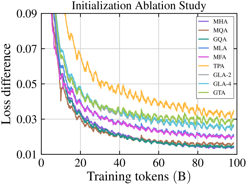
Figure 1: Loss difference between $N(0,σ=0.02)$ and zero initialization, calculated by subtracting the loss of the latter from the former.
<details>
<summary>2603.02188v1/x2.png Details</summary>
### Visual Description
## Line Graph: Scale Ablation Study
### Overview
The chart illustrates the relationship between training tokens (x-axis) and loss difference (y-axis) for three model configurations: MLA (blue), GLA-2 (gray), and MLRA-2 (orange). All three lines show distinct trends in loss reduction over 100 training tokens.
### Components/Axes
- **X-axis**: Training tokens (B) ranging from 0 to 100 in increments of 20.
- **Y-axis**: Loss difference (0.000 to 0.010) in logarithmic scale.
- **Legend**:
- Blue: MLA
- Gray: GLA-2
- Orange: MLRA-2
- **Grid**: Light gray gridlines for reference.
### Detailed Analysis
1. **MLA (Blue Line)**:
- Starts at ~0.002 loss difference at 0 tokens.
- Sharp decline to ~0.0015 at ~10 tokens.
- Stabilizes between 0.0015–0.0025 for remaining tokens.
- Final value at 100 tokens: ~0.0022.
2. **GLA-2 (Gray Line)**:
- Begins at ~0.008 loss difference.
- Gradual decline to ~0.006 by ~40 tokens.
- Fluctuates between 0.006–0.007 for remaining tokens.
- Final value at 100 tokens: ~0.0062.
3. **MLRA-2 (Orange Line)**:
- Starts at ~0.008 loss difference.
- Sharp drop to ~0.0055 by ~20 tokens.
- Stabilizes between 0.0055–0.0065 for remaining tokens.
- Final value at 100 tokens: ~0.0064.
### Key Observations
- **MLA** exhibits the most rapid initial improvement but plateaus at a higher loss difference than GLA-2/MLRA-2.
- **GLA-2** and **MLRA-2** show similar trajectories but diverge slightly in final performance (MLRA-2 ends marginally better).
- All models stabilize after ~40 tokens, suggesting diminishing returns in loss reduction beyond this point.
### Interpretation
The data suggests that:
1. **MLA** prioritizes early-stage optimization but may lack efficiency in later training phases.
2. **GLA-2** and **MLRA-2** demonstrate more balanced improvement, with MLRA-2 achieving marginally better final performance.
3. The convergence of GLA-2 and MLRA-2 lines implies similar architectural efficacy, while MLA's distinct trajectory highlights a different optimization strategy.
4. The logarithmic y-axis emphasizes early-stage performance differences, which diminish as training progresses.
*Note: Values are approximate due to the absence of explicit data points. Trends are inferred from line trajectories and relative positioning.*
</details>
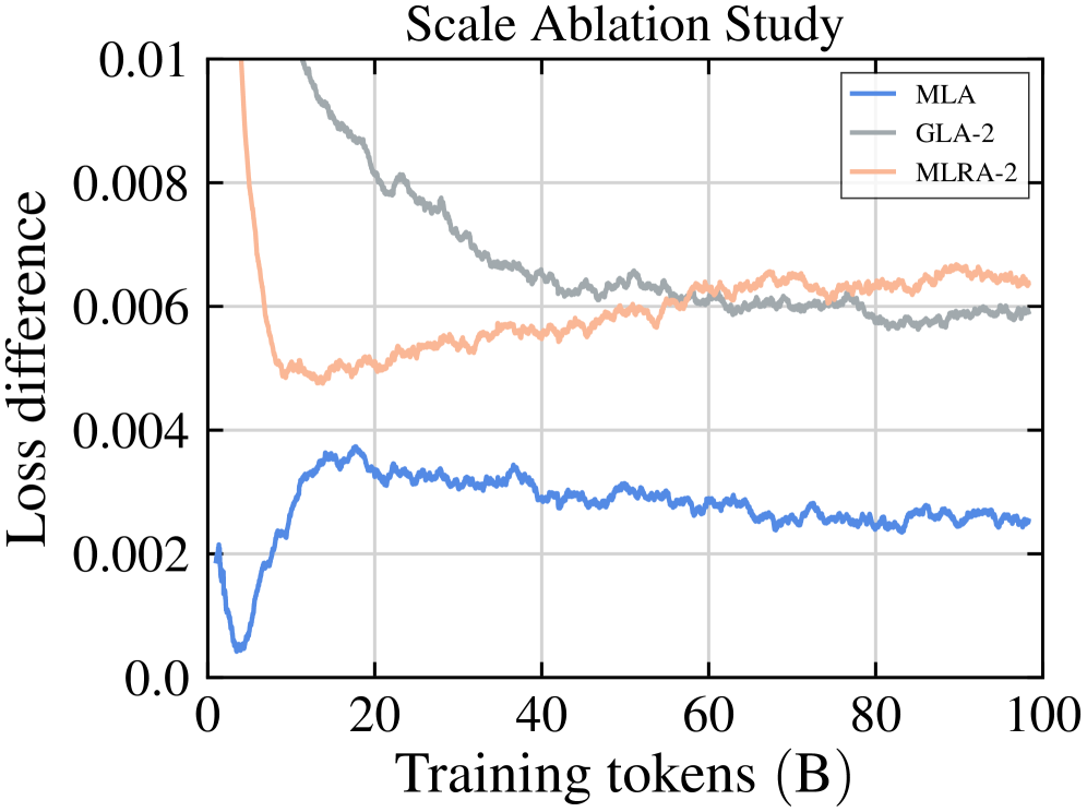
Figure 2: Loss difference between models without and with scaling, calculated by subtracting the loss of the latter from the former.
<details>
<summary>2603.02188v1/x3.png Details</summary>
### Visual Description
## Line Chart: Double Heads Ablation Study
### Overview
The chart compares the loss difference of three models (GQA, MLA, GLA-2) during training, measured across 100 billion training tokens. Loss difference is plotted on a logarithmic scale (0.000 to 0.01), with training tokens on a linear scale (0 to 100B). All three models show distinct trends in loss convergence.
### Components/Axes
- **X-axis**: Training tokens (B) – linear scale from 0 to 100B, marked at 20, 40, 60, 80, 100.
- **Y-axis**: Loss difference – logarithmic scale from 0.000 to 0.01, marked at 0.002, 0.004, 0.006, 0.008, 0.01.
- **Legend**: Located in the top-left corner, associating:
- Teal line: GQA
- Blue line: MLA
- Gray line: GLA-2
### Detailed Analysis
1. **GQA (Teal)**:
- Starts at ~0.01 loss difference at 0 tokens.
- Sharp decline to ~0.002 by 20 tokens.
- Gradual increase to ~0.006 by 100 tokens, with minor fluctuations.
2. **MLA (Blue)**:
- Begins at ~0.006 loss difference at 0 tokens.
- Decreases to ~0.004 by 20 tokens.
- Steady rise to ~0.008 by 100 tokens, with consistent oscillations.
3. **GLA-2 (Gray)**:
- Starts at ~0.004 loss difference at 0 tokens.
- Drops to ~0.002 by 20 tokens.
- Remains stable between 0.002–0.003 for the remainder of training.
### Key Observations
- **Initial Divergence**: GQA exhibits the highest initial loss but converges fastest (~0.002 by 20 tokens).
- **Long-term Behavior**: MLA shows the most significant late-stage increase in loss difference, suggesting potential overfitting or instability.
- **Stability**: GLA-2 maintains the lowest and most consistent loss difference after 20 tokens.
### Interpretation
The data suggests GLA-2 achieves the most stable training performance, with minimal loss difference fluctuations. MLA’s late-stage increase in loss difference may indicate suboptimal generalization, while GQA’s rapid early convergence followed by a rebound hints at possible architectural trade-offs. The logarithmic y-axis emphasizes early-stage differences, highlighting GQA’s initial superiority before plateauing. These trends could reflect differences in model architecture, optimization strategies, or regularization techniques.
</details>
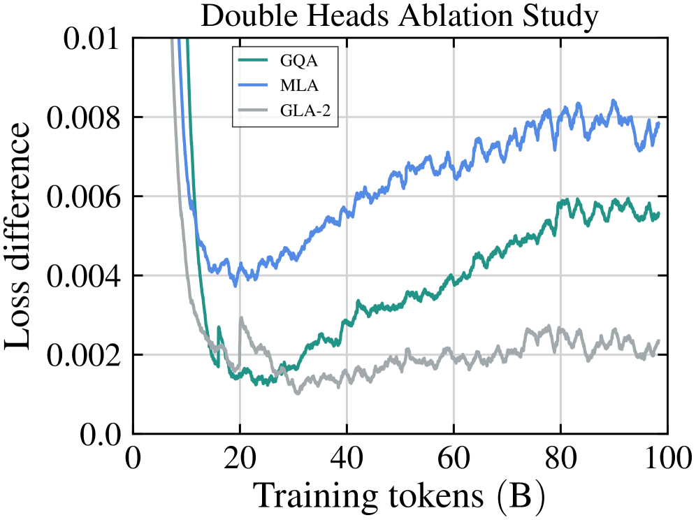
Figure 3: Loss difference between models with and without double heads, calculated by subtracting the loss of the latter from the former.
<details>
<summary>2603.02188v1/x4.png Details</summary>
### Visual Description
## Line Graph: Gating Ablation Study
### Overview
The chart illustrates the relationship between training tokens (B) and loss difference across five gating mechanisms: GQA, MLA, GLA-2, MLRA-2, and MLRA-4. All lines originate near 0.018 loss difference at 0 tokens and exhibit distinct decay patterns as training tokens increase to 100.
### Components/Axes
- **X-axis**: Training tokens (B) [0, 20, 40, 60, 80, 100]
- **Y-axis**: Loss difference [0.003, 0.006, 0.009, 0.012, 0.015, 0.018]
- **Legend**: Located in top-right corner with color-coded labels:
- Teal: GQA
- Blue: MLA
- Gray: GLA-2
- Orange: MLRA-2
- Red: MLRA-4
### Detailed Analysis
1. **GQA (Teal)**:
- Starts at ~0.018 loss difference
- Gradual linear decline to ~0.012 by 100 tokens
- Maintains highest loss difference throughout
2. **MLA (Blue)**:
- Sharp initial drop from ~0.018 to ~0.009 in first 20 tokens
- Slower decay to ~0.007 by 100 tokens
- Second-highest loss difference after GQA
3. **GLA-2 (Gray)**:
- Steep decline from ~0.018 to ~0.008 in first 20 tokens
- Gradual decay to ~0.006 by 100 tokens
- Third-highest loss difference
4. **MLRA-2 (Orange)**:
- Sharp drop from ~0.018 to ~0.009 in first 20 tokens
- Slower decay to ~0.007 by 100 tokens
- Overlaps with MLA after 40 tokens
5. **MLRA-4 (Red)**:
- Steepest initial drop from ~0.018 to ~0.008 in first 20 tokens
- Rapid decay to ~0.006 by 40 tokens
- Lowest loss difference by 100 tokens (~0.005)
### Key Observations
- All methods show rapid initial loss reduction (first 20 tokens)
- GQA maintains consistently higher loss difference than other methods
- MLRA-4 demonstrates fastest convergence to lowest loss difference
- Lines converge toward similar values after 60 tokens
- No outliers or anomalies detected
### Interpretation
The data suggests that gating mechanism architecture significantly impacts loss reduction efficiency during training. MLRA-4's steepest decay curve indicates superior early-stage performance, while GQA's sustained higher loss difference may reflect different optimization characteristics. The convergence of lines after 60 tokens implies diminishing returns on gating mechanism effectiveness beyond mid-training stages. These findings could inform architectural choices for balancing training speed and model performance in sequence modeling tasks.
</details>
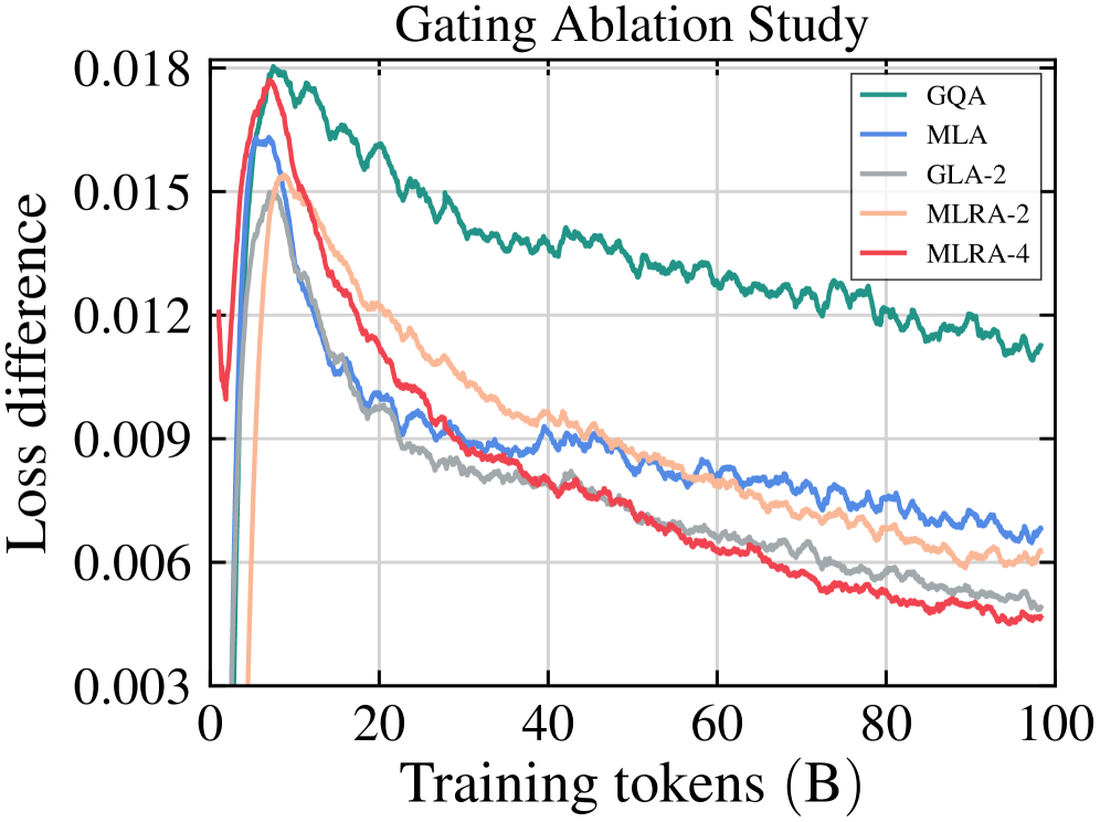
Figure 4: Loss difference between models without and with gating, calculated by subtracting the loss of the latter from the former.
#### 4.2.1 Initialization
We follow the GPT (Radford et al., 2018) initialization method, where all model weights are initialized using an $N(0,σ=0.02)$ distribution. However, TPA employs zero initialization for the output projection parameters of the attention and FFN modules, which is an approach also explored in muP (Yang et al., 2021) and LoRA (Hu et al., 2022). To evaluate these different approaches, we conduct an ablation study comparing zero initialization against $N(0,σ=0.02)$ for the output projection parameters across all models. It is important to note that for MLA, GLA-2, and GLA-4, we apply scaling as discussed in Section 3.3. As illustrated in Figure 4 and Table 38, the results for loss and perplexity demonstrate that zero initialization outperforms the $N(0,σ=0.02)$ distribution. Unless otherwise specified, all models in the following experiments utilize this zero initialization.
#### 4.2.2 Scaling
We evaluate the effectiveness of the scaling on MLA, GLA-2, and MLRA-2. As illustrated in Figure 4, all three models exhibit improved convergence when scaling is applied. As shown in Table 39, all three models achieve lower average perplexity after scaling. Notably, MLA and GLA-2 show more substantial improvements, while MLRA-2 yields a marginal gain. Unless otherwise specified, MLA, GLA, and MLRA in the following experiments utilize this scaling.
#### 4.2.3 Double Heads
While MLRA-2 and MLRA-4 do not increase the number of query heads, their multi-branch design increases the number of attention heads involved in computation. Consequently, we double the number of attention heads for GQA, MLA, and GLA-2 while keeping the KV-cache size fixed to evaluate whether this increase contributes to performance gains. To maintain a constant parameter budget during this adjustment, we reduce the FFN intermediate sizes; the corresponding architectural hyperparameters are detailed in Appendix F.4. As illustrated by the loss curves in Figure 4 and the results in Table 40, doubling the number of attention heads leads to higher loss and fails to decrease perplexity across all three models. These findings suggest that doubling the number of attention heads does not yield any measurable performance improvement. Unless otherwise specified, GQA, MLA, and GLA use the default head count (no head doubling).
Table 3: Validation perplexity (lower is better) across seven datasets: Wikipedia, C4, Pile, RefinedWeb, Cosmopedia, FineWeb, and FineWeb-Edu. The best results are indicated in bold, while the second best are underlined.
| Method MHA MQA | Wikipedia 14.624 15.134 | C4 16.575 16.837 | Pile 12.929 14.008 | RefinedWeb 18.698 19.202 | Cosmopedia 9.102 9.484 | FineWeb 15.656 15.942 | FineWeb-Edu 9.434 9.533 | Avg 13.860 14.306 |
| --- | --- | --- | --- | --- | --- | --- | --- | --- |
| GQA | 15.057 | 16.628 | 13.758 | 18.885 | 9.504 | 15.713 | 9.427 | 14.139 |
| MLA | 14.567 | 16.345 | 12.965 | 18.523 | 8.966 | 15.440 | 9.284 | 13.727 |
| MFA | 15.693 | 16.738 | 13.903 | 19.125 | 9.423 | 15.815 | 9.506 | 14.315 |
| TPA | 14.789 | 16.622 | 13.333 | 18.971 | 9.130 | 15.717 | 9.333 | 13.985 |
| GLA-2 | 14.605 | 16.323 | 13.225 | 18.509 | 9.118 | 15.424 | 9.249 | 13.779 |
| GLA-4 | 14.547 | 16.436 | 13.229 | 18.578 | 9.076 | 15.535 | 9.307 | 13.815 |
| GTA | 14.733 | 16.599 | 13.402 | 18.924 | 9.129 | 15.672 | 9.346 | 13.972 |
| MLRA-2 | 14.615 | 16.342 | 13.236 | 18.602 | 9.153 | 15.439 | 9.242 | 13.804 |
| MLRA-4 | 14.407 | 16.286 | 13.124 | 18.398 | 8.937 | 15.361 | 9.193 | 13.672 |
Table 4: Downstream evaluation on seven common-sense reasoning benchmarks: ARC-E, ARC-C, OpenBookQA, BoolQ, HellaSwag, Winogrande, and PIQA. ARC-E/C, OpenBookQA, HellaSwag, and PIQA use normalized accuracy (%); others use standard accuracy (%). Best is bold; second best is underlined.
| Method MHA MQA | ARC-E 69.11 66.16 | ARC-C 39.16 38.31 | OpenBookQA 40.80 41.80 | BoolQ 62.26 62.05 | HellaSwag 60.82 60.24 | Winogrande 57.62 59.83 | PIQA 74.86 74.48 | Avg 57.81 57.55 |
| --- | --- | --- | --- | --- | --- | --- | --- | --- |
| GQA | 67.13 | 39.42 | 42.00 | 63.39 | 61.29 | 56.91 | 75.08 | 57.89 |
| MLA | 68.22 | 39.16 | 42.60 | 64.10 | 61.39 | 60.06 | 75.68 | 58.75 |
| MFA | 69.02 | 39.93 | 42.40 | 63.49 | 60.72 | 58.96 | 75.19 | 58.53 |
| TPA | 69.44 | 40.61 | 41.60 | 60.03 | 61.02 | 57.85 | 74.54 | 57.87 |
| GLA-2 | 68.01 | 40.19 | 40.60 | 63.94 | 61.54 | 58.41 | 75.41 | 58.30 |
| GLA-4 | 68.77 | 41.04 | 41.20 | 61.96 | 61.61 | 58.09 | 74.65 | 58.19 |
| GTA | 67.97 | 39.68 | 42.60 | 59.72 | 61.03 | 58.48 | 75.14 | 57.80 |
| MLRA-2 | 67.89 | 42.24 | 42.00 | 61.65 | 61.49 | 59.98 | 75.52 | 58.68 |
| MLRA-4 | 67.63 | 41.38 | 43.00 | 61.74 | 62.16 | 61.48 | 74.48 | 58.84 |
Table 5: Validation perplexity (lower is better) w/ gating across seven datasets. The best results are indicated in bold, while the second best are underlined.
| Method GQA w/ gating MLA w/ gating | Wikipedia 14.362 14.346 | C4 16.484 16.297 | Pile 13.113 12.866 | RefinedWeb 18.696 18.456 | Cosmopedia 9.098 8.936 | FineWeb 15.581 15.383 | FineWeb-Edu 9.311 9.212 | Avg 13.806 13.642 |
| --- | --- | --- | --- | --- | --- | --- | --- | --- |
| GLA-2 w/ gating | 14.597 | 16.286 | 12.997 | 18.473 | 8.986 | 15.369 | 9.198 | 13.701 |
| MLRA-2 w/ gating | 14.424 | 16.252 | 13.017 | 18.407 | 8.924 | 15.351 | 9.180 | 13.651 |
| MLRA-4 w/ gating | 14.431 | 16.170 | 13.073 | 18.386 | 8.874 | 15.266 | 9.148 | 13.621 |
### 4.3 Main Results
As shown in Table 3, MLRA-4 achieves the best average perplexity (13.672), outperforming all other models, including MLA (13.727). Notably, MLRA-4 also delivers the lowest perplexity on FineWeb-Edu (9.193). Furthermore, Table 4 demonstrates that MLRA-4 attains the highest average zero-shot accuracy across all common-sense reasoning tasks. This consistent superiority of MLRA-4 over MLRA-2 across both evaluations highlights the benefits of increasing the number of branches.
### 4.4 Gated Attention
Following Qiu et al. (2025), we introduce a gating mechanism prior to the attention output projection (Appendix E). To maintain a constant parameter budget, we reduce the FFN intermediate size accordingly; detailed architectural hyperparameters are provided in Appendix F.5. As illustrated in Figure 4, all five models exhibit improved convergence with gating applied. As shown in Table 5, gating consistently improves perplexity across all models, with MLRA-4 achieving the best overall average perplexity and MLRA-2 attaining performance comparable to MLA (13.651 vs. 13.642).
<details>
<summary>2603.02188v1/x5.png Details</summary>
### Visual Description
## Line Chart: Decoding Latency
### Overview
The chart illustrates the relationship between sequence length (K) and decoding latency (µs) for four different methods: GQA (TP=8), MLA (DP), GLA-2 (TP=2), and MLRA-4 (TP=4). Latency increases with sequence length for all methods, but the rate of increase varies significantly.
### Components/Axes
- **X-axis**: Sequence Length (K)
- Scale: 0 to 2048 (logarithmic-like increments: 256, 512, 768, 1024, 1280, 1536, 1792, 2048)
- **Y-axis**: Latency (µs)
- Scale: 0 to 900
- **Legend**: Top-left corner, with color-coded labels:
- Teal: GQA (TP=8)
- Blue: MLA (DP)
- Gray: GLA-2 (TP=2)
- Red: MLRA-4 (TP=4)
### Detailed Analysis
1. **MLA (DP)**:
- **Trend**: Steepest upward slope, consistently highest latency.
- **Data Points**:
- At 256K: ~150 µs
- At 2048K: ~900 µs
- **Uncertainty**: ±10% due to linear extrapolation between marked points.
2. **GQA (TP=8)**:
- **Trend**: Moderate upward slope, second-highest latency.
- **Data Points**:
- At 256K: ~50 µs
- At 2048K: ~350 µs
- **Uncertainty**: ±5% based on consistent spacing between points.
3. **GLA-2 (TP=2)**:
- **Trend**: Gradual upward slope, third-highest latency.
- **Data Points**:
- At 256K: ~75 µs
- At 2048K: ~450 µs
- **Uncertainty**: ±3% due to tightly clustered points.
4. **MLRA-4 (TP=4)**:
- **Trend**: Shallowest upward slope, lowest latency.
- **Data Points**:
- At 256K: ~25 µs
- At 2048K: ~300 µs
- **Uncertainty**: ±2% with minimal deviation between points.
### Key Observations
- **Latency Hierarchy**: MLA (DP) > GQA (TP=8) > GLA-2 (TP=2) > MLRA-4 (TP=4) across all sequence lengths.
- **Scalability**: MLA (DP) exhibits poor scalability, with latency increasing ~6x from 256K to 2048K. MLRA-4 scales more efficiently (~12x increase).
- **TP Impact**: Higher TP values (e.g., GQA TP=8 vs. GLA-2 TP=2) correlate with higher latency, suggesting trade-offs between parallelism and overhead.
### Interpretation
The data suggests that MLA (DP) is the least efficient method for decoding long sequences, likely due to algorithmic complexity or suboptimal resource utilization. In contrast, MLRA-4 (TP=4) achieves the lowest latency, indicating superior optimization for scalability. The TP parameter appears to influence latency, with higher TP values increasing overhead. These trends highlight the importance of method selection based on sequence length and hardware constraints.
</details>
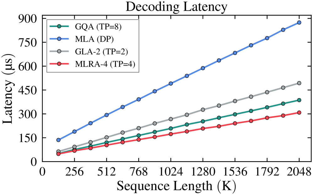
Figure 5: Decoding latency (lower is better) versus sequence length (batch=1) for GQA, MLA, GLA-2, and MLRA-4.
<details>
<summary>2603.02188v1/x6.png Details</summary>
### Visual Description
## Line Chart: Decoding Throughput
### Overview
The chart compares the decoding throughput (tokens/ms) of four algorithms (GQA, MLA, GLA-2, MLRA-4) across sequence lengths (0–16K). Throughput decreases for all algorithms as sequence length increases, with varying rates of decline.
### Components/Axes
- **X-axis**: Sequence Length (K), ranging from 0 to 16 in increments of 2.
- **Y-axis**: Throughput (tokens/ms), ranging from 150 to 900 in increments of 150.
- **Legend**: Located in the top-right corner, mapping colors/markers to algorithms:
- Green circles: GQA (TP=8)
- Blue circles: MLA (DP=8)
- Gray circles: GLA-2 (TP=2, DP=4)
- Red circles: MLRA-4 (TP=4, DP=2)
### Detailed Analysis
1. **GQA (TP=8)**:
- Starts at ~850 tokens/ms at sequence length 0.
- Drops sharply to ~600 tokens/ms at sequence length 2.
- Continues declining steeply, reaching ~150 tokens/ms at sequence length 16.
- **Trend**: Steepest decline among all algorithms.
2. **MLA (DP=8)**:
- Begins at ~600 tokens/ms at sequence length 0.
- Declines gradually to ~400 tokens/ms at sequence length 16.
- **Trend**: Moderate, linear decrease.
3. **GLA-2 (TP=2, DP=4)**:
- Starts at ~550 tokens/ms at sequence length 0.
- Declines slowly to ~350 tokens/ms at sequence length 16.
- **Trend**: Gradual, near-linear decrease.
4. **MLRA-4 (TP=4, DP=2)**:
- Begins at ~800 tokens/ms at sequence length 0.
- Drops to ~450 tokens/ms at sequence length 10.
- Stabilizes slightly before declining to ~400 tokens/ms at sequence length 16.
- **Trend**: Initial sharp drop, then gradual decline.
### Key Observations
- **GQA** exhibits the most significant throughput degradation with increasing sequence length.
- **MLRA-4** maintains higher throughput than other algorithms after the initial drop, suggesting better scalability.
- **MLA** and **GLA-2** show similar performance patterns but with MLA starting slightly higher.
- No lines intersect after sequence length 2, indicating stable performance hierarchies.
### Interpretation
The data suggests that algorithm efficiency varies with sequence length and parameter configurations (TP/DP). GQA’s steep decline implies high computational overhead for longer sequences, while MLRA-4’s resilience indicates optimized handling of extended contexts. Parameters like TP (token processing) and DP (depth) likely influence scalability differently across architectures. The chart highlights trade-offs between algorithm design and performance under varying workloads.
</details>
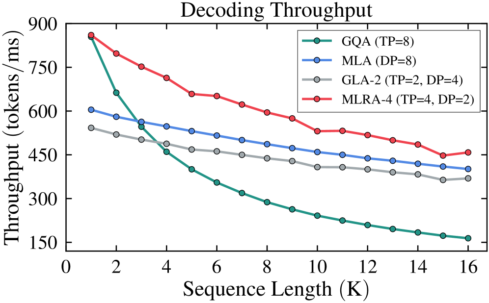
Figure 6: Decoding throughput versus sequence length (batch=128) for GQA, MLA, GLA-2, and MLRA-4.
### 4.5 Decoding Efficiency
Decoding Speed.
We benchmark long-context attention decoding speed for GQA, MLA, GLA-2, and MLRA-4 on an NVIDIA H100 80GB GPU. For MLA, GLA-2, and MLRA-4, we follow the attention decoding formulation in Eq. (1). All models use 64 heads with a head dimension of 128; for MLA, GLA-2, and MLRA-4, the partial RoPE dimension is 64. MLA is evaluated using DeepSeek’s official implementation FlashMLA (Jiashi Li, 2025). GQA and GLA-2 use FlashAttention-3 kernels (Dao et al., 2022; Dao, 2024; Shah et al., 2024). We implement our MLRA-4 kernel based on FlashAttention-3. We evaluate decoding speed across sequence lengths from 131,072 to 2,097,152 tokens (128K–2M). As shown in Figure 6, MLRA-4 consistently outperforms all baselines at every length, yielding 1.05 $×$ –1.26 $×$ speedups over GQA. The gap grows with context length against GQA and GLA-2, while the speedup over MLA remains steady at about 2.8 $×$ , indicating that MLRA-4 with TP=4 substantially reduces long-context decoding latency.
Decoding Throughput.
We evaluate decoding throughput for GQA, MLA, GLA-2, and MLRA-4 on eight NVIDIA H100 80GB GPUs, fixing the number of attention heads to 128 and the hidden size to 7168, following DeepSeekV3 (DeepSeek and others, 2024b). We set $g=16$ for GQA. For MLA decoding deployment, there is a trade-off between data parallelism (DP) and tensor parallelism. With DP, we assign different requests to different devices, so attention parameters are replicated across devices and the load can become imbalanced due to varying sequence lengths. With TP, the up-projection parameters are sharded by head, but the KV cache loading is repeated across devices. Following SGLang (Zheng et al., 2024), we aim to eliminate redundant KV cache loading. Therefore, we use DP=8 for MLA, TP=2/DP=4 for GLA-2, TP=4/DP=2 for MLRA-4, and TP=8 for GQA. Throughput is reported for sequence lengths ranging from 1,024 to 16,384 tokens, and our end-to-end measurements include both the pre-attention stage that prepares inputs for the attention kernel and the attention computation itself. We accelerate pre-attention computation with torch.compile (Paszke et al., 2019) for MLA, GLA-2, and MLRA-4, and with custom Triton kernels for GQA. As shown in Figure 6, MLRA-4 achieves the highest decoding throughput across both short and long sequence lengths. This suggests that MLRA-4 with TP=4/DP=2 reduces parameter redundancy relative to MLA’s DP=8, while introducing only modest partial RoPE duplication, thereby yielding higher throughput than MLA. For short sequences, GQA outperforms MLA and GLA-2 because pre-attention dominates latency. However, MLRA-4 remains competitive with GQA due to having even fewer query, key, and value parameters, as shown in Appendix F.1.
## 5 Conclusion
We propose Multi-Head Low-Rank Attention (MLRA), a novel attention mechanism with native 4-way tensor parallelism support. At the 2.9B scale, MLRA-4 achieves state-of-the-art performance on perplexity and zero-shot common-sense reasoning benchmarks. Furthermore, MLRA achieves the lowest decoding latency for long-context sequences (up to 2M tokens) and the highest throughput across sequence lengths from 1K to 16K tokens with 4-way tensor parallelism.
## Acknowledgement
We thank Songlin Yang for helpful discussion. We thank all the anonymous reviewers for their helpful comments and suggestions.
## References
- J. Ainslie, J. Lee-Thorp, M. de Jong, Y. Zemlyanskiy, F. Lebron, and S. Sanghai (2023) GQA: training generalized multi-query transformer models from multi-head checkpoints. In Empirical Methods in Natural Language Processing, Cited by: Table 1, §4.1.
- S. Anagnostidis, D. Pavllo, L. Biggio, L. Noci, A. Lucchi, and T. Hofmann (2023) Dynamic context pruning for efficient and interpretable autoregressive transformers. In Advances in Neural Information Processing Systems, Cited by: Appendix I.
- M. Beck, K. Pöppel, M. Spanring, A. Auer, O. Prudnikova, M. Kopp, G. Klambauer, J. Brandstetter, and S. Hochreiter (2024) Xlstm: extended long short-term memory. In Advances in Neural Information Processing Systems, Cited by: Appendix I.
- L. Ben Allal, A. Lozhkov, G. Penedo, T. Wolf, and L. von Werra (2024) Cosmopedia. Hugging Face. Note: https://huggingface.co/datasets/HuggingFaceTB/cosmopedia Cited by: §4.1.
- Y. Bisk, R. Zellers, R. L. Bras, J. Gao, and Y. Choi (2020) Piqa: reasoning about physical commonsense in natural language. In AAAI Conference on Artificial Intelligence, Cited by: §4.1.
- R. Cai, Y. Tian, Z. Wang, and B. Chen (2024) LoCoCo: dropping in convolutions for long context compression. In International Conference on Machine Learning, Cited by: Appendix I.
- C. Chang, W. Lin, C. Lin, C. Chen, Y. Hu, P. Wang, N. Huang, L. Ceze, M. S. Abdelfattah, and K. Wu (2025) Palu: KV-cache compression with low-rank projection. In International Conference on Learning Representations, Cited by: Appendix I.
- R. Chen, Z. Wang, B. Cao, T. Wu, S. Zheng, X. Li, X. Wei, S. Yan, M. Li, and Y. Liang (2024a) ArkVale: efficient generative LLM inference with recallable key-value eviction. In Advances in Neural Information Processing Systems, Cited by: Appendix I.
- Y. Chen, S. Qian, H. Tang, X. Lai, Z. Liu, S. Han, and J. Jia (2024b) LongLoRA: efficient fine-tuning of long-context large language models. In International Conference on Learning Representations, Cited by: Appendix I.
- C. Clark, K. Lee, M. Chang, T. Kwiatkowski, M. Collins, and K. Toutanova (2019) BoolQ: exploring the surprising difficulty of natural yes/no questions. In North American Association for Computational Linguistics, Cited by: §4.1.
- T. Dao, D. Y. Fu, S. Ermon, A. Rudra, and C. Re (2022) FlashAttention: fast and memory-efficient exact attention with IO-awareness. In Advances in Neural Information Processing Systems, Cited by: Appendix I, §4.5.
- T. Dao and A. Gu (2024) Transformers are SSMs: generalized models and efficient algorithms through structured state space duality. In International Conference on Machine Learning, Cited by: Appendix I.
- T. Dao (2024) FlashAttention-2: faster attention with better parallelism and work partitioning. In International Conference on Learning Representations, Cited by: Appendix I, §4.5.
- DeepSeek et al. (2024a) Deepseek-v2: a strong, economical, and efficient mixture-of-experts language model. arXiv preprint arXiv:2405.04434. Cited by: §1, Table 1, §4.1.
- DeepSeek et al. (2024b) DeepSeek-v3 technical report. arXiv preprint arXiv:2412.19437. Cited by: §4.5.
- DeepSeek et al. (2024c) DeepSeek-v3 technical report. GitHub. Note: https://github.com/deepseek-ai/DeepSeek-V3 Cited by: §2.1, §2.1.
- T. Dettmers, A. Pagnoni, A. Holtzman, and L. Zettlemoyer (2023) Qlora: efficient finetuning of quantized llms. In Advances in Neural Information Processing Systems, Cited by: Appendix I.
- R. Dey and F. M. Salem (2017) Gate-variants of gated recurrent unit (gru) neural networks. In International Midwest Symposium on Circuits and Systems, Cited by: §F.5.
- H. Dong, X. Yang, Z. Zhang, Z. Wang, Y. Chi, and B. Chen (2024) Get more with less: synthesizing recurrence with kv cache compression for efficient llm inference. In International Conference on Machine Learning, Cited by: Appendix I.
- F. Fuchs, D. Worrall, V. Fischer, and M. Welling (2020) Se (3)-transformers: 3d roto-translation equivariant attention networks. In Advances in Neural Information Processing Systems, Cited by: §B.1.
- L. Gao, S. Biderman, S. Black, L. Golding, T. Hoppe, C. Foster, J. Phang, H. He, A. Thite, N. Nabeshima, S. Presser, and C. Leahy (2020) The pile: an 800gb dataset of diverse text for language modeling. arXiv preprint arXiv:2101.00027. Cited by: §4.1.
- L. Gao, J. Tow, B. Abbasi, S. Biderman, S. Black, A. DiPofi, C. Foster, L. Golding, J. Hsu, A. Le Noac’h, H. Li, K. McDonell, N. Muennighoff, C. Ociepa, J. Phang, L. Reynolds, H. Schoelkopf, A. Skowron, L. Sutawika, E. Tang, A. Thite, B. Wang, K. Wang, and A. Zou (2024) A framework for few-shot language model evaluation. Cited by: §4.1.
- S. Ge, Y. Zhang, L. Liu, M. Zhang, J. Han, and J. Gao (2024) Model tells you what to discard: adaptive KV cache compression for LLMs. In International Conference on Learning Representations, Cited by: Appendix I.
- A. Gholami, Z. Yao, S. Kim, C. Hooper, M. W. Mahoney, and K. Keutzer (2024) AI and memory wall. IEEE Micro. Cited by: §1.
- A. Gu and T. Dao (2024) Mamba: linear-time sequence modeling with selective state spaces. In Conference on Language Modeling, Cited by: Appendix I.
- A. Gu, K. Goel, and C. Re (2022) Efficiently modeling long sequences with structured state spaces. In International Conference on Learning Representations, Cited by: Appendix I.
- J. He and J. Zhai (2024) Fastdecode: high-throughput gpu-efficient llm serving using heterogeneous pipelines. arXiv preprint arXiv:2403.11421. Cited by: §1.
- S. Hochreiter and J. Schmidhuber (1997) Long short-term memory. Neural Computation. Cited by: §F.5.
- C. R. C. Hooper, S. Kim, H. Mohammadzadeh, M. W. Mahoney, S. Shao, K. Keutzer, and A. Gholami (2024) KVQuant: towards 10 million context length LLM inference with KV cache quantization. In Advances in Neural Information Processing Systems, Cited by: Appendix I.
- E. J. Hu, Y. Shen, P. Wallis, Z. Allen-Zhu, Y. Li, S. Wang, L. Wang, and W. Chen (2022) LoRA: low-rank adaptation of large language models. In International Conference on Learning Representations, Cited by: Appendix I, §4.2.1.
- J. Hu, H. Li, Y. Zhang, Z. Wang, S. Zhou, X. Zhang, H. Shum, and D. Jiang (2024) Multi-matrix factorization attention. arXiv preprint arXiv:2412.19255. Cited by: §1, Table 1, §4.1.
- A. Ivanov, N. Dryden, T. Ben-Nun, S. Li, and T. Hoefler (2021) Data movement is all you need: a case study on optimizing transformers. In Machine Learning and Systems, Cited by: §1.
- H. Jiang, Y. Li, C. Zhang, Q. Wu, X. Luo, S. Ahn, Z. Han, A. H. Abdi, D. Li, C. Lin, Y. Yang, and L. Qiu (2024) MInference 1.0: accelerating pre-filling for long-context LLMs via dynamic sparse attention. In Advances in Neural Information Processing Systems, Cited by: Appendix I.
- S. L. Jiashi Li (2025) FlashMLA: efficient mla decoding kernels. GitHub. Note: https://github.com/deepseek-ai/FlashMLA Cited by: Appendix I, §2.1, §3.4, §4.5.
- A. Karpathy (2022) NanoGPT. GitHub. Note: https://github.com/karpathy/nanoGPT Cited by: §4.1.
- A. Katharopoulos, A. Vyas, N. Pappas, and F. Fleuret (2020) Transformers are rnns: fast autoregressive transformers with linear attention. In International Conference on Machine Learning, Cited by: Appendix I.
- J. Kim, J. Yeom, S. Yun, and H. O. Song (2024) Compressed context memory for online language model interaction. In International Conference on Learning Representations, Cited by: Appendix I.
- W. Kwon, Z. Li, S. Zhuang, Y. Sheng, L. Zheng, C. H. Yu, J. Gonzalez, H. Zhang, and I. Stoica (2023) Efficient memory management for large language model serving with pagedattention. In Symposium on Operating Systems Principles, Cited by: Appendix I.
- P. Lewis, E. Perez, A. Piktus, F. Petroni, V. Karpukhin, N. Goyal, H. Kuttler, M. Lewis, W. Yih, T. Rocktäschel, S. Riedel, and D. Kiela (2020) Retrieval-augmented generation for knowledge-intensive nlp tasks. In Advances in Neural Information Processing Systems, Cited by: §1.
- Y. Li, Y. Huang, B. Yang, B. Venkitesh, A. Locatelli, H. Ye, T. Cai, P. Lewis, and D. Chen (2024) SnapKV: LLM knows what you are looking for before generation. In Advances in Neural Information Processing Systems, Cited by: Appendix I.
- V. Lialin, S. Muckatira, N. Shivagunde, and A. Rumshisky (2024) ReLoRA: high-rank training through low-rank updates. In International Conference on Learning Representations, Cited by: Appendix I.
- C. Lin, S. Gao, J. S. Smith, A. Patel, S. Tuli, Y. Shen, H. Jin, and Y. Hsu (2025) MoDeGPT: modular decomposition for large language model compression. In International Conference on Learning Representations, Cited by: Appendix I.
- Y. Liu, H. Li, Y. Cheng, S. Ray, Y. Huang, Q. Zhang, K. Du, J. Yao, S. Lu, G. Ananthanarayanan, M. Maire, H. Hoffmann, A. Holtzman, and J. Jiang (2024a) Cachegen: kv cache compression and streaming for fast large language model serving. In ACM Special Interest Group on Data Communication, Cited by: Appendix I.
- Z. Liu, A. Desai, F. Liao, W. Wang, V. Xie, Z. Xu, A. Kyrillidis, and A. Shrivastava (2023) Scissorhands: exploiting the persistence of importance hypothesis for LLM KV cache compression at test time. In Advances in Neural Information Processing Systems, Cited by: Appendix I.
- Z. Liu, J. Yuan, H. Jin, S. Zhong, Z. Xu, V. Braverman, B. Chen, and X. Hu (2024b) KIVI: a tuning-free asymmetric 2bit quantization for KV cache. In International Conference on Machine Learning, Cited by: Appendix I.
- Llama et al. (2024) The llama 3 herd of models. arXiv preprint arXiv:2407.21783. Cited by: §4.1.
- M. LongCat et al. (2025) Longcat-flash technical report. arXiv preprint arXiv:2509.01322. Cited by: §3.3, §3.3, §3.3.
- I. Loshchilov and F. Hutter (2017) SGDR: stochastic gradient descent with warm restarts. In International Conference on Learning Representations, Cited by: §4.1.
- I. Loshchilov and F. Hutter (2019) Decoupled weight decay regularization. In International Conference on Learning Representations, Cited by: §4.1.
- S. Malladi, A. Wettig, D. Yu, D. Chen, and S. Arora (2023) A kernel-based view of language model fine-tuning. In International Conference on Machine Learning, Cited by: Appendix I.
- F. Meng, P. Tang, X. Tang, Z. Yao, X. Sun, and M. Zhang (2025) Transmla: multi-head latent attention is all you need. In Advances in Neural Information Processing Systems, Cited by: Appendix I.
- T. Mihaylov, P. Clark, T. Khot, and A. Sabharwal (2018) Can a suit of armor conduct electricity? a new dataset for open book question answering. In Empirical Methods in Natural Language Processing, Cited by: §4.1.
- P. Nawrot, A. Łańcucki, M. Chochowski, D. Tarjan, and E. Ponti (2024) Dynamic memory compression: retrofitting LLMs for accelerated inference. In International Conference on Machine Learning, Cited by: Appendix I.
- OpenAI et al. (2024) OpenAI o1 system card. arXiv preprint arXiv:2412.16720. Cited by: §1.
- A. Paszke, S. Gross, F. Massa, A. Lerer, J. Bradbury, G. Chanan, T. Killeen, Z. Lin, N. Gimelshein, L. Antiga, A. Desmaison, A. Köpf, E. Yang, Z. DeVito, M. Raison, A. Tejani, S. Chilamkurthy, B. Steiner, L. Fang, J. Bai, and S. Chintala (2019) Pytorch: an imperative style, high-performance deep learning library. In Advances in Neural Information Processing Systems, Cited by: §4.5.
- G. Penedo, H. Kydlíček, L. B. allal, A. Lozhkov, M. Mitchell, C. Raffel, L. V. Werra, and T. Wolf (2024) The fineweb datasets: decanting the web for the finest text data at scale. In Advances in Neural Information Processing Systems Datasets and Benchmarks Track, Cited by: §4.1, §4.1.
- G. Penedo, Q. Malartic, D. Hesslow, R. Cojocaru, H. Alobeidli, A. Cappelli, B. Pannier, E. Almazrouei, and J. Launay (2023) The refinedweb dataset for falcon LLM: outperforming curated corpora with web data only. In Advances in Neural Information Processing Systems Datasets and Benchmarks Track, Cited by: §4.1.
- B. Peng, D. Goldstein, Q. G. Anthony, A. Albalak, E. Alcaide, S. Biderman, E. Cheah, T. Ferdinan, K. K. GV, H. Hou, S. Krishna, R. M. Jr., N. Muennighoff, F. Obeid, A. Saito, G. Song, H. Tu, R. Zhang, B. Zhao, Q. Zhao, J. Zhu, and R. Zhu (2024) Eagle and finch: RWKV with matrix-valued states and dynamic recurrence. In Conference on Language Modeling, Cited by: Appendix I.
- H. Peng, N. Pappas, D. Yogatama, R. Schwartz, N. Smith, and L. Kong (2021) Random feature attention. In International Conference on Learning Representations, Cited by: Appendix I.
- Z. Qin, S. Yang, and Y. Zhong (2023) Hierarchically gated recurrent neural network for sequence modeling. In Advances in Neural Information Processing Systems, Cited by: Appendix I.
- Z. Qiu, Z. Wang, B. Zheng, Z. Huang, K. Wen, S. Yang, R. Men, L. Yu, F. Huang, S. Huang, D. Liu, J. Zhou, and J. Lin (2025) Gated attention for large language models: non-linearity, sparsity, and attention-sink-free. In Advances in Neural Information Processing Systems, Cited by: §F.5, §4.4.
- A. Radford, K. Narasimhan, T. Salimans, and I. Sutskever (2018) Improving language understanding by generative pre-training. OpenAI Technical Report. Cited by: §4.2.1.
- C. Raffel, N. Shazeer, A. Roberts, K. Lee, S. Narang, M. Matena, Y. Zhou, W. Li, and P. J. Liu (2020) Exploring the limits of transfer learning with a unified text-to-text transformer. Journal of Machine Learning Research. Cited by: §4.1.
- R. Sadhukhan, J. Chen, Z. Chen, V. Tiwari, R. Lai, J. Shi, I. E. Yen, A. May, T. Chen, and B. Chen (2025) MagicDec: breaking the latency-throughput tradeoff for long context generation with speculative decoding. In International Conference on Learning Representations, Cited by: §1.
- K. Sakaguchi, R. L. Bras, C. Bhagavatula, and Y. Choi (2021) Winogrande: an adversarial winograd schema challenge at scale. Communications of the ACM. Cited by: §4.1.
- V. G. Satorras, E. Hoogeboom, and M. Welling (2021) E (n) equivariant graph neural networks. In International Conference on Machine Learning, Cited by: §B.1.
- I. Schlag, K. Irie, and J. Schmidhuber (2021) Linear transformers are secretly fast weight programmers. In International Conference on Machine Learning, Cited by: Appendix I.
- J. Shah, G. Bikshandi, Y. Zhang, V. Thakkar, P. Ramani, and T. Dao (2024) FlashAttention-3: fast and accurate attention with asynchrony and low-precision. In Advances in Neural Information Processing Systems, Cited by: Appendix I, §2.1, §4.5.
- N. Shazeer (2019) Fast transformer decoding: one write-head is all you need. arXiv preprint arXiv:1911.02150. Cited by: §1, Table 1, §4.1.
- J. T.H. Smith, A. Warrington, and S. Linderman (2023) Simplified state space layers for sequence modeling. In International Conference on Learning Representations, Cited by: Appendix I.
- R. K. Srivastava, K. Greff, and J. Schmidhuber (2015) Highway networks. arXiv preprint arXiv:1505.00387. Cited by: §F.5.
- J. Su, M. Ahmed, Y. Lu, S. Pan, W. Bo, and Y. Liu (2024) Roformer: enhanced transformer with rotary position embedding. Neurocomputing. Cited by: §B.2, §2.1.
- H. Sun, L. Chang, W. Bao, S. Zheng, N. Zheng, X. Liu, H. Dong, Y. Chi, and B. Chen (2025) ShadowKV: KV cache in shadows for high-throughput long-context LLM inference. In International Conference on Machine Learning, Cited by: Appendix I.
- Y. Sun, L. Dong, S. Huang, S. Ma, Y. Xia, J. Xue, J. Wang, and F. Wei (2023) Retentive network: a successor to transformer for large language models. arXiv preprint arXiv:2307.08621. Cited by: Appendix I.
- Y. Sun, L. Dong, Y. Zhu, S. Huang, W. Wang, S. Ma, Q. Zhang, J. Wang, and F. Wei (2024) You only cache once: decoder-decoder architectures for language models. In Advances in Neural Information Processing Systems, Cited by: Appendix I.
- J. Tang, Y. Zhao, K. Zhu, G. Xiao, B. Kasikci, and S. Han (2024) QUEST: query-aware sparsity for efficient long-context LLM inference. In International Conference on Machine Learning, Cited by: Appendix I.
- X. Tang, F. Meng, P. Tang, Y. Wang, D. Yin, X. Sun, and M. Zhang (2025) TPLA: tensor parallel latent attention for efficient disaggregated prefill & decode inference. In International Conference on Architectural Support for Programming Languages and Operating Systems, Cited by: Appendix I.
- K. Team et al. (2025) Kimi k2: open agentic intelligence. arXiv preprint arXiv:2507.20534. Cited by: §3.4.
- A. Vaswani, N. M. Shazeer, N. Parmar, J. Uszkoreit, L. Jones, A. N. Gomez, L. Kaiser, and I. Polosukhin (2017) Attention is all you need. In Advances in Neural Information Processing Systems, Cited by: §1, Table 1, §4.1.
- X. Wang, Y. Zheng, Z. Wan, and M. Zhang (2025) SVD-LLM: truncation-aware singular value decomposition for large language model compression. In International Conference on Learning Representations, Cited by: Appendix I.
- J. Wei, X. Wang, D. Schuurmans, M. Bosma, F. Xia, E. Chi, Q. V. Le, and D. Zhou (2022) Chain-of-thought prompting elicits reasoning in large language models. In Advances in Neural Information Processing Systems, Cited by: §1.
- M. Weiler, M. Geiger, M. Welling, W. Boomsma, and T. S. Cohen (2018) 3d steerable cnns: learning rotationally equivariant features in volumetric data. In Advances in Neural Information Processing Systems, Cited by: §B.1.
- S. Williams, A. Waterman, and D. Patterson (2009) Roofline: an insightful visual performance model for multicore architectures. Communications of the ACM. Cited by: §3.4.
- G. Xiao, J. Tang, J. Zuo, junxian guo, S. Yang, H. Tang, Y. Fu, and S. Han (2025) DuoAttention: efficient long-context LLM inference with retrieval and streaming heads. In International Conference on Learning Representations, Cited by: Appendix I.
- G. Xiao, Y. Tian, B. Chen, S. Han, and M. Lewis (2024) Efficient streaming language models with attention sinks. In International Conference on Learning Representations, Cited by: Appendix I.
- V. Yadav, S. Bethard, and M. Surdeanu (2019) Quick and (not so) dirty: unsupervised selection of justification sentences for multi-hop question answering. In Empirical Methods in Natural Language Processing, Cited by: §4.1.
- A. Yang, A. Li, B. Yang, B. Zhang, B. Hui, B. Zheng, B. Yu, C. Gao, C. Huang, C. Lv, C. Zheng, D. Liu, F. Zhou, F. Huang, F. Hu, H. Ge, H. Wei, H. Lin, J. Tang, J. Yang, J. Tu, J. Zhang, J. Yang, J. Yang, J. Zhou, J. Zhou, J. Lin, K. Dang, K. Bao, K. Yang, L. Yu, L. Deng, M. Li, M. Xue, M. Li, P. Zhang, P. Wang, Q. Zhu, R. Men, R. Gao, S. Liu, S. Luo, T. Li, T. Tang, W. Yin, X. Ren, X. Wang, X. Zhang, X. Ren, Y. Fan, Y. Su, Y. Zhang, Y. Zhang, Y. Wan, Y. Liu, Z. Wang, Z. Cui, Z. Zhang, Z. Zhou, and Z. Qiu (2025a) Qwen3 technical report. arXiv preprint arXiv:2505.09388. Cited by: §3.4.
- B. Yang, B. Venkitesh, D. Gnaneshwar, H. Lin, D. Cairuz, P. Blunsom, and A. Locatelli (2025b) Rope to nope and back again: a new hybrid attention strategy. In Advances in Neural Information Processing Systems, Cited by: §1.
- G. Yang, E. J. Hu, I. Babuschkin, S. Sidor, X. Liu, D. Farhi, N. Ryder, J. Pachocki, W. Chen, and J. Gao (2021) Tuning large neural networks via zero-shot hyperparameter transfer. In Advances in Neural Information Processing Systems, Cited by: §4.2.1.
- S. Yang, J. Kautz, and A. Hatamizadeh (2025c) Gated delta networks: improving mamba2 with delta rule. In International Conference on Learning Representations, Cited by: Appendix I.
- S. Yang, B. Wang, Y. Shen, R. Panda, and Y. Kim (2024a) Gated linear attention transformers with hardware-efficient training. In International Conference on Machine Learning, Cited by: Appendix I.
- S. Yang, B. Wang, Y. Zhang, Y. Shen, and Y. Kim (2024b) Parallelizing linear transformers with the delta rule over sequence length. In Advances in Neural Information Processing Systems, Cited by: Appendix I.
- T. Zadouri, H. Strauss, and T. Dao (2025) Hardware-efficient attention for fast decoding. In Conference on Language Modeling, Cited by: §1, §1, §2.2, §3.4, Table 1, Table 1, Table 1, §4.1.
- R. Zellers, A. Holtzman, Y. Bisk, A. Farhadi, and Y. Choi (2019) Hellaswag: can a machine really finish your sentence?. In Association for Computational Linguistics, Cited by: §4.1.
- Y. Zeng and K. Lee (2024) The expressive power of low-rank adaptation. In International Conference on Learning Representations, Cited by: Appendix I.
- B. Zhang and R. Sennrich (2019) Root mean square layer normalization. In Advances in Neural Information Processing Systems, Cited by: §3.3.
- Q. Zhang, M. Chen, A. Bukharin, P. He, Y. Cheng, W. Chen, and T. Zhao (2023a) Adaptive budget allocation for parameter-efficient fine-tuning. In International Conference on Learning Representations, Cited by: Appendix I.
- Y. Zhang, Y. Liu, H. Yuan, Z. Qin, Y. Yuan, Q. Gu, and A. C. Yao (2025) Tensor product attention is all you need. In Advances in Neural Information Processing Systems, Cited by: §1, Table 1, Table 1, §4.1.
- Y. Zhang, S. Yang, R. Zhu, Y. Zhang, L. Cui, Y. Wang, B. Wang, F. Shi, B. Wang, W. Bi, P. Zhou, and G. Fu (2024a) Gated slot attention for efficient linear-time sequence modeling. In Advances in Neural Information Processing Systems, Cited by: Appendix I.
- Y. Zhang, Y. Du, G. Luo, Y. Zhong, Z. Zhang, S. Liu, and R. Ji (2024b) CaM: cache merging for memory-efficient LLMs inference. In International Conference on Machine Learning, Cited by: Appendix I.
- Z. Zhang, Y. Sheng, T. Zhou, T. Chen, L. Zheng, R. Cai, Z. Song, Y. Tian, C. Re, C. Barrett, Z. Wang, and B. Chen (2023b) H2O: heavy-hitter oracle for efficient generative inference of large language models. In Advances in Neural Information Processing Systems, Cited by: Appendix I.
- C. Zheng, J. Sun, Y. Gao, Y. Wang, P. Wang, J. Xiong, L. Ren, H. Cheng, J. Kulkarni, Y. Shen, A. Wang, M. Schwager, A. Schneider, X. Liu, and J. Gao (2025) SAS: simulated attention score. In Advances in Neural Information Processing Systems, Cited by: §1.
- L. Zheng, L. Yin, Z. Xie, C. Sun, J. Huang, C. H. Yu, S. Cao, C. Kozyrakis, I. Stoica, J. E. Gonzalez, C. Barrett, and Y. Sheng (2024) SGLang: efficient execution of structured language model programs. In Advances in Neural Information Processing Systems, Cited by: §4.5.
- J. Zhu, K. Greenewald, K. Nadjahi, H. S. D. O. Borde, R. B. Gabrielsson, L. Choshen, M. Ghassemi, M. Yurochkin, and J. Solomon (2024) Asymmetry in low-rank adapters of foundation models. In International Conference on Machine Learning, Cited by: Appendix I.
## Appendix A Notation
Table 6: Notation used throughout this paper.
| $n$ | scalar | Sequence length (number of tokens). |
| --- | --- | --- |
| $d$ | scalar | Model/hidden dimension. |
| $h$ | scalar | Number of attention heads. |
| $d_h$ | scalar | Per-head dimension. |
| $d_h^R$ | scalar | Partial RoPE dimension. |
| $d_r$ | scalar | RoPE rotation dimension in Theorem 1 (even); typically $d_r=d_h$ or $d_r=d_h^R$ . |
| $d_f$ | scalar | MLP intermediate (FFN) dimension. |
| $g$ | scalar | Number of groups (or KV heads in MQA/GQA). |
| $r$ | scalar | Repeat factor $r=h/g$ when $g$ KV heads are broadcast to $h$ query heads. |
| $α_q,α_kv,α_attn$ | scalar | Variance-calibrating rescaling factors for query/KV latents and attention outputs. |
| $β_q,β_kv$ | scalar | Number of low-rank components in TPA for queries / keys-values. |
| $d_c$ | scalar | Latent KV dimension in MLA/GLA. |
| $d_c^\prime$ | scalar | Latent Q dimension in MLA/GLA/MFA. |
| $s$ | integer | Translation offset. |
| $t_q,t_k$ | integer | Query/key token positions. |
| $b$ | integer | Block index. |
| $i$ | integer | Head index ( $i∈\{0, …, h-1\}$ ). |
| $j$ | integer | Group index ( $j∈\{0, …, g-1\}$ ). |
| $γ(i)$ | integer | Mapping from head index to group index. |
| $\bar{i}$ | integer | Head index within group in GLA-2, $\bar{i}=i-γ(i)h/2$ . |
| $τ$ | scalar | Softmax scaling factor, $τ=1/√{d_h+d_h^R}$ . |
| $φ$ | integer | Number of tensor-parallel devices. |
| $≤ft(·\right)$ | function | Rotary Position Embedding applied to vectors (implemented via rotation matrices). |
| $≤ft(·\right)$ | function | Root-mean-square normalization. |
| $≤ft(·\right)$ | operator | Tensor reshaping (no data change). |
| $≤ft(·\right)$ | operator | Replication along the head dimension (e.g., broadcasting $g$ KV heads to $h$ heads). |
| $≤ft(·\right)$ | operator | Concatenation along the last dimension unless stated otherwise. |
## Appendix B Theorem
### B.1 Translation Equivariance
Equivariance is a fundamental property in geometric systems such as molecules, where vector features such as atomic forces or dipole moments must transform consistently with the coordinate system (Weiler et al., 2018; Fuchs et al., 2020; Satorras et al., 2021). In the context of sequence models, a common transformation is sequence translation. Let $\bm{X}=≤ft(\bm{x}^(0),\bm{x}^(1),…,\bm{x}^(n-1)\right)∈X$ be a sequence of tokens, and define a translation operator $T_s:X→X$ that translates the entire sequence by $s$ positions. Let $φ:X→Y$ be a function that maps a sequence to a matrix of attention scores $φ≤ft(\bm{X}\right)∈ℝ^n× n$ , where each element $φ≤ft(\bm{X}\right)_t_{q,t_k}=A≤ft(\bm{x}^(t_q),\bm{x}^(t_k)\right)$ denotes the attention score between tokens $\bm{x}^(t_q)$ and $\bm{x}^(t_k)$ . We say that $φ$ is translation equivariant if there exists a corresponding output-space transformation $S_s:Y→Y$ such that:
$$
φ≤ft(T_s≤ft(\bm{X}\right)\right)=S_s≤ft(φ≤ft(\bm{X}\right)\right), ∀ s. \tag{11}
$$
This property ensures that the attention score between two tokens depends only on their relative positions, not their absolute positions. That is crucial for batch inference using left padding, where sequences of different lengths are offset to align ends. The first non-padding token of a sequence is no longer at position $0$ , yet attention scores remain equivariant to this translation.
### B.2 Rotary Position Embedding
Rotary Position Embedding (RoPE) (Su et al., 2024) is a positional encoding method designed to incorporate relative position information directly into the attention mechanism. We show in this section that RoPE is translation equivariant.
**Theorem 1**
*Given two tokens with query $\bm{q}$ and key $\bm{k}$ at positions $t_q$ and $t_k$ , respectively, let $≤ft(\bm{q},t_q\right)$ and $≤ft(\bm{k},t_k\right)$ denote the RoPE-encoded vectors. We show that translating both positions by an offset $s$ leaves the inner product unchanged:
$$
≤ft⟨≤ft(\bm{q},t_q+s\right),≤ft(\bm{k},t_k+s\right)\right⟩=≤ft⟨≤ft(\bm{q},t_q\right),≤ft(\bm{k},t_k\right)\right⟩.
$$
Equivalently, for the attention-score matrix $φ(\bm{X})∈ℝ^n× n$ induced by RoPE-based dot products, $φ$ is translation equivariant in the sense of Eq. (11) with $S_s$ being the simultaneous row/column shift operator.*
* Proof*
Let the RoPE dimension be $d_r$ (assumed even). RoPE applies a block-diagonal rotation matrix $\bm{R}_t∈ℝ^d_r× d_r$ at position $t$ . Writing RoPE as right-multiplication on row vectors, we compute the inner product under RoPE as:
$$
≤ft(\bm{q}\bm{R}_t_{q}\right)≤ft(\bm{k}\bm{R}_t_{k}\right)^⊤=\bm{q}\bm{R}_t_{q}\bm{R}_t_{k}^⊤\bm{k}^⊤=≤ft[∑_\ell=0^d_r/2-1\bm{q}_≤ft[2\ell:2\ell+2\right] \bm{k}_≤ft[2\ell:2\ell+2\right]^* e^i≤ft(t_q-t_k\right)θ_\ell\right],
$$
where $θ_\ell$ is the angular frequency for the $\ell$ -th 2D block and $(·)^*$ denotes complex conjugation under the standard $ℝ^2≃ℂ$ identification. Now consider translating both tokens by an offset $s$ . The relative displacement is unchanged:
$$
≤ft(t_q+s\right)-≤ft(t_k+s\right)=t_q-t_k,
$$
so the factor $e^i≤ft(t_q-t_k\right)θ_\ell$ remains unchanged for every $\ell$ . Therefore,
$$
≤ft⟨≤ft(\bm{q},t_q+s\right),≤ft(\bm{k},t_k+s\right)\right⟩=≤ft⟨≤ft(\bm{q},t_q\right),≤ft(\bm{k},t_k\right)\right⟩.
$$
This proves RoPE-induced dot-product scores satisfy translation equivariance in Eq. (11). ∎
**Remark 2**
*While RoPE preserves dot-product translation equivariance, applying an arbitrary linear map after RoPE generally breaks this property. Specifically, consider:
$$
≤ft⟨≤ft(\bm{q},t_q\right)\bm{W}^Q, ≤ft(\bm{k},t_k\right)\bm{W}^K\right⟩=\bm{q}\bm{R}_t_{q}\bm{W}^Q≤ft(\bm{W}^K\right)^⊤\bm{R}_t_{k}^⊤\bm{k}^⊤.
$$
The term $\bm{W}^Q≤ft(\bm{W}^K\right)^⊤$ breaks translation equivariance by disrupting the expression’s dependence on the relative position $t_q-t_k$ . The property would only be preserved in the specific case where $\bm{W}^Q≤ft(\bm{W}^K\right)^⊤=\bm{I}$ , which would reduce the expression to its original form. However, since this constraint is difficult to enforce during training, translation equivariance is generally lost when applying a linear projection after RoPE.*
## Appendix C Attention Mechanism
### C.1 Multi-Head Attention (MHA)
Consider a sequence of $n$ tokens with hidden states $\bm{H}∈ℝ^n× d$ . We first project these hidden states into queries, keys, and values using projection matrices $\bm{W}^Q,\bm{W}^K,\bm{W}^V∈ℝ^d×≤ft(hd_h\right)$ :
$$
\overline{\bm{Q}}=≤ft(\bm{H}\bm{W}^Q\right), \overline{\bm{K}}=≤ft(\bm{H}\bm{W}^K\right), \overline{\bm{V}}=\bm{H}\bm{W}^V,
$$
where $\overline{\bm{Q}},\overline{\bm{K}},\overline{\bm{V}}∈ℝ^n×≤ft(hd_h\right)$ , $h$ is the number of attention heads, and $d_h$ is the dimensionality of each head. Next, we reshape these matrices to separate the head dimension:
$$
\bm{\mathsfit{Q}}=≤ft(\overline{\bm{Q}}, ≤ft[n, h, d_h\right]\right), \bm{\mathsfit{K}}^C=≤ft(\overline{\bm{K}}, ≤ft[n, h, d_h\right]\right), \bm{\mathsfit{V}}^C=≤ft(\overline{\bm{V}}, ≤ft[n, h, d_h\right]\right),
$$
such that $\bm{\mathsfit{Q}},\bm{\mathsfit{K}}^C,\bm{\mathsfit{V}}^C∈ℝ^n× h× d_h$ . We cache $\bm{\mathsfit{K}}^C$ and $\bm{\mathsfit{V}}^C$ to accelerate inference.
**Remark 3**
*Let $\bm{\mathsfit{Q}},\bm{\mathsfit{K}}^C∈ℝ^n× h× d_h$ denote the RoPE-encoded queries and keys after projection and reshaping. For head $i$ , define:
$$
\bm{\mathsfit{Q}}_t_{q,i,:}:=\bm{\mathsfit{Q}}≤ft[t_q, i, :\right], \bm{\mathsfit{K}}_t_{k,i,:}:=\bm{\mathsfit{K}}^C≤ft[t_k, i, :\right].
$$
Then, for any translation offset $s$ , it follows from Theorem 1 that:
$$
≤ft⟨\bm{\mathsfit{Q}}_t_{q+s,i,:}, \bm{\mathsfit{K}}_t_{k+s,i,:}\right⟩=≤ft⟨\bm{\mathsfit{Q}}_t_{q,i,:}, \bm{\mathsfit{K}}_t_{k,i,:}\right⟩.
$$*
### C.2 Multi-Query Attention (MQA) and Grouped-Query Attention (GQA)
Both MQA and GQA reduce the number of key and value heads compared to MHA, while maintaining the full number of query heads. MQA takes this to the extreme by using a single key-value head for all query heads, whereas GQA partitions the query heads into groups that each share a key-value head. Given a sequence of $n$ tokens with hidden states $\bm{H}∈ℝ^n× d$ , the queries are computed using the same projection as in MHA. To reduce KV cache, we use projection matrices $\bm{W}^K,\bm{W}^V∈ℝ^d× d_hg$ , where $g<h$ (e.g., $g=1$ for MQA), to compute:
$$
\overline{\bm{K}}^C=≤ft(\bm{H}\bm{W}^K\right), \overline{\bm{V}}^C=\bm{H}\bm{W}^V.
$$
These are then reshaped into per-head form:
$$
\bm{\mathsfit{K}}^C=≤ft(\overline{\bm{K}}^C, ≤ft[n, g, d_h\right]\right), \bm{\mathsfit{V}}^C=≤ft(\overline{\bm{V}}^C, ≤ft[n, g, d_h\right]\right).
$$
We cache $\bm{\mathsfit{K}}^C$ and $\bm{\mathsfit{V}}^C$ during inference. We repeat them by a factor of $r=h/g$ along the head axis to match the $h$ query heads:
$$
\begin{split}\bm{\mathsfit{K}}&=≤ft(\bm{\mathsfit{K}}^C, r, dim=1\right)∈ℝ^n× h× d_h,\\
\bm{\mathsfit{V}}&=≤ft(\bm{\mathsfit{V}}^C, r, dim=1\right)∈ℝ^n× h× d_h.\end{split}
$$
**Remark 4**
*Let $\bm{\mathsfit{Q}}∈ℝ^n× h× d_h$ and $\bm{\mathsfit{K}}^C∈ℝ^n× g× d_h$ denote the RoPE-encoded queries and cached keys, respectively. For head $i$ , define:
$$
\bm{\mathsfit{Q}}_t_{q,i,:}:=\bm{\mathsfit{Q}}≤ft[t_q, i, :\right], \bm{\mathsfit{K}}_t_{k,i,:}:=\bm{\mathsfit{K}}^C≤ft[t_k, ≤ft\lfloor\frac{i}{r}\right\rfloor, :\right].
$$
Since both vectors are RoPE-encoded, for any offset $s$ (with valid indices),
$$
≤ft⟨\bm{\mathsfit{Q}}_t_{q+s,i,:}, \bm{\mathsfit{K}}_t_{k+s,i,:}\right⟩=≤ft⟨\bm{\mathsfit{Q}}_t_{q,i,:}, \bm{\mathsfit{K}}_t_{k,i,:}\right⟩.
$$*
### C.3 Multi-Head Latent Attention (MLA)
Given a sequence of $n$ tokens with hidden states $\bm{H}∈ℝ^n× d$ , MLA first computes queries as:
$$
\begin{split}\bm{C}^Q=α_q≤ft(\bm{H}\bm{W}^DQ\right), \overline{\bm{Q}}^NoPE&=\bm{C}^Q\bm{W}^UQ, \overline{\bm{Q}}^RoPE=≤ft(\bm{C}^Q\bm{W}^QR\right),\\
\bm{W}^DQ∈ℝ^d× d_c^{\prime}, \bm{W}^UQ&∈ℝ^d_c^{\prime×≤ft(hd_h\right)}, \bm{W}^QR∈ℝ^d_c^{\prime×(hd_h^R)}.\end{split}
$$
where $α_q=√{\frac{d}{d_c^\prime}}$ is the rescaling factor for query states $\bm{C}^Q$ . We then reshape queries to separate heads:
$$
\bm{\mathsfit{Q}}^NoPE=≤ft(\overline{\bm{Q}}^NoPE, ≤ft[n, h, d_h\right]\right), \bm{\mathsfit{Q}}^RoPE=≤ft(\overline{\bm{Q}}^RoPE, ≤ft[n, h, d_h^R\right]\right),
$$
where $\bm{\mathsfit{Q}}^NoPE∈ℝ^n× h× d_h$ and $\bm{\mathsfit{Q}}^RoPE∈ℝ^n× h× d_h^{R}$ . These are concatenated along the last dimension to form the final query:
$$
\bm{\mathsfit{Q}}=≤ft(≤ft[\bm{\mathsfit{Q}}^NoPE, \bm{\mathsfit{Q}}^RoPE\right], dim=2\right).
$$
To reduce the KV cache, MLA obtains shared compressed KV states via a down-projection:
$$
\begin{split}\bm{C}^KV=α_kv≤ft(\bm{H}\bm{W}^DKV\right), &\bm{W}^DKV∈ℝ^d× d_c,\\
\bm{K}^RoPE=≤ft(\bm{H}\bm{W}^KR\right), &\bm{W}^KR∈ℝ^d× d_h^{R},\end{split}
$$
where $α_kv=√{\frac{d}{d_c}}$ . Both $\bm{C}^KV$ and $\bm{K}^RoPE$ are cached during inference. MLA computes $h$ keys and values using learnable up-projection matrices:
$$
\overline{\bm{K}}^NoPE=\bm{C}^KV\bm{W}^UK, \overline{\bm{V}}=\bm{C}^KV\bm{W}^UV, \bm{W}^UK,\bm{W}^UV∈ℝ^d_c×≤ft(hd_h\right).
$$
These are reshaped into per-head form:
$$
\begin{split}\bm{\mathsfit{K}}^NoPE=≤ft(\overline{\bm{K}}^NoPE, ≤ft[n, h, d_h\right]\right)&, \bm{\mathsfit{K}}^RoPE=≤ft(\bm{K}^RoPE, ≤ft[n, 1, d_h^R\right]\right),\\
\bm{\mathsfit{V}}=&≤ft(\overline{\bm{V}}, ≤ft[n, h, d_h\right]\right),\end{split}
$$
where $\bm{\mathsfit{K}}^NoPE∈ℝ^n× h× d_h$ and $\bm{\mathsfit{V}}∈ℝ^n× h× d_h$ .
To obtain per-head position-aware keys, MLA repeats the partial RoPE key across heads:
$$
\bm{\mathsfit{K}}=≤ft(≤ft[\bm{\mathsfit{K}}^NoPE, ≤ft(\bm{\mathsfit{K}}^RoPE, h, dim=1\right)\right], dim=2\right).
$$
**Remark 5**
*We analyze the translation equivariance property of MLA. Let $\bm{\mathsfit{Q}}_t_{q,i,:}=≤ft(\bm{\mathsfit{Q}}^NoPE≤ft[t_q, i, :\right], \bm{\mathsfit{Q}}^RoPE≤ft[t_q, i, :\right]\right)$ and $\bm{\mathsfit{K}}_t_{k,i,:}=≤ft(\bm{\mathsfit{K}}^NoPE≤ft[t_k, i, :\right], \bm{K}^RoPE≤ft[t_k, :\right]\right)$ denote the query and key vectors for head $i$ at positions $t_q$ and $t_k$ , respectively. The attention score for this head is given by the inner product:
$$
≤ft⟨\bm{\mathsfit{Q}}_t_{q,i,:}, \bm{\mathsfit{K}}_t_{k,i,:}\right⟩=≤ft⟨\bm{\mathsfit{Q}}^NoPE≤ft[t_q, i, :\right], \bm{\mathsfit{K}}^NoPE≤ft[t_k, i, :\right]\right⟩+≤ft⟨\bm{\mathsfit{Q}}^RoPE≤ft[t_q, i, :\right], \bm{\mathsfit{K}}^RoPE≤ft[t_k, :\right]\right⟩.
$$
Between the two terms, the second term with RoPE is position-dependent yet translation equivariant, due to Theorem 1. The first term is position-independent and thus unchanged under joint translations of $t_q$ and $t_k$ . Therefore, the attention score $≤ft⟨\bm{\mathsfit{Q}}_t_{q,i,:}, \bm{\mathsfit{K}}_t_{k,i,:}\right⟩$ is equivariant to translation in input positions. Although MLA introduces positional inductive bias via partial RoPE and is translation equivariant, we refer to this property as semi-translation equivariance to distinguish it from full RoPE translation equivariance.*
### C.4 Multi-matrix Factorization Attention (MFA)
Given a sequence of $n$ tokens with hidden states $\bm{H}∈ℝ^n× d$ , MFA uses $h$ query heads but only a single shared key-value head (i.e., $g=1$ ). MFA first projects $\bm{H}$ to a low-rank space and applies RMSNorm:
$$
\bm{C}^Q=≤ft(\bm{H}\bm{W}^CQ\right), \bm{W}^CQ∈ℝ^d× d_c^{\prime}.
$$
It then up-projects to all query heads and applies RoPE:
$$
\overline{\bm{Q}}=≤ft(\bm{C}^Q\bm{W}^UQ\right), \bm{W}^UQ∈ℝ^d_c^{\prime×(h· 2d_h)}.
$$
Finally, we reshape into per-head form:
$$
\bm{\mathsfit{Q}}=≤ft(\overline{\bm{Q}}, ≤ft[n, h, 2d_h\right]\right)∈ℝ^n× h× 2d_h.
$$
To reduce KV cache, MFA computes only one key head and one value head:
$$
\overline{\bm{K}}^C=≤ft(\bm{H}\bm{W}^K\right), \overline{\bm{V}}^C=\bm{H}\bm{W}^V, \bm{W}^K,\bm{W}^V∈ℝ^d× 2d_h,
$$
where $\overline{\bm{K}}^C,\overline{\bm{V}}^C∈ℝ^n× 2d_h$ . We reshape them as
$$
\bm{\mathsfit{K}}^C=≤ft(\overline{\bm{K}}^C, ≤ft[n, 1, 2d_h\right]\right), \bm{\mathsfit{V}}^C=≤ft(\overline{\bm{V}}^C, ≤ft[n, 1, 2d_h\right]\right),
$$
and cache $\bm{\mathsfit{K}}^C$ and $\bm{\mathsfit{V}}^C$ during inference. We repeat them along the head axis to match the $h$ query heads:
$$
\begin{split}\bm{\mathsfit{K}}&=≤ft(\bm{\mathsfit{K}}^C, h, dim=1\right)∈ℝ^n× h× 2d_h,\\
\bm{\mathsfit{V}}&=≤ft(\bm{\mathsfit{V}}^C, h, dim=1\right)∈ℝ^n× h× 2d_h.\end{split}
$$
The analysis of translation equivariance is similar to that of MQA.
### C.5 Tensor Product Attention (TPA)
TPA achieves KV cache compression through low-rank factorization. It represents each head’s key/value at a token as a low-rank mixture of $β_kv$ components: component vectors in $ℝ^d_h$ and head-specific scalar coefficients. During inference, TPA caches the component tensors and coefficient tensors, and computes keys/values on the fly via linear combination.
Given a sequence of $n$ tokens with hidden states $\bm{H}∈ℝ^n× d$ , TPA first computes the query/key/value factors:
$$
\begin{split}\overline{\bm{Q}}^A&=\bm{H}\bm{W}^AQ, \bm{W}^AQ∈ℝ^d×(β_qh), \overline{\bm{Q}}^A∈ℝ^n×(β_qh),\\
\overline{\bm{Q}}^C&=\bm{H}\bm{W}^CQ, \bm{W}^CQ∈ℝ^d×(β_qd_h), \overline{\bm{Q}}^C∈ℝ^n×(β_qd_h),\\
\overline{\bm{K}}^A&=\bm{H}\bm{W}^AK, \bm{W}^AK∈ℝ^d×(β_kvh), \overline{\bm{K}}^A∈ℝ^n×(β_kvh),\\
\overline{\bm{K}}^C&=\bm{H}\bm{W}^CK, \bm{W}^CK∈ℝ^d×(β_kvd_h), \overline{\bm{K}}^C∈ℝ^n×(β_kvd_h),\\
\overline{\bm{V}}^A&=\bm{H}\bm{W}^AV, \bm{W}^AV∈ℝ^d×(β_kvh), \overline{\bm{V}}^A∈ℝ^n×(β_kvh),\\
\overline{\bm{V}}^C&=\bm{H}\bm{W}^CV, \bm{W}^CV∈ℝ^d×(β_kvd_h), \overline{\bm{V}}^C∈ℝ^n×(β_kvd_h).\end{split}
$$
We reshape the projections into 3D tensors:
$$
\begin{split}\bm{\mathsfit{Q}}^A&=≤ft(\overline{\bm{Q}}^A, ≤ft[n, β_q, h\right]\right),\\
\bm{\mathsfit{Q}}^C&=≤ft(≤ft(\overline{\bm{Q}}^C, ≤ft[n, β_q, d_h\right]\right)\right),\\
\bm{\mathsfit{K}}^A&=≤ft(\overline{\bm{K}}^A, ≤ft[n, β_kv, h\right]\right),\\
\bm{\mathsfit{K}}^C&=≤ft(≤ft(\overline{\bm{K}}^C, ≤ft[n, β_kv, d_h\right]\right)\right),\\
\bm{\mathsfit{V}}^A&=≤ft(\overline{\bm{V}}^A, ≤ft[n, β_kv, h\right]\right),\\
\bm{\mathsfit{V}}^C&=≤ft(\overline{\bm{V}}^C, ≤ft[n, β_kv, d_h\right]\right),\end{split}
$$
so that $\bm{\mathsfit{Q}}^A∈ℝ^n×β_q× h$ , $\bm{\mathsfit{Q}}^C∈ℝ^n×β_q× d_h$ , $\bm{\mathsfit{K}}^A∈ℝ^n×β_kv× h$ , $\bm{\mathsfit{K}}^C∈ℝ^n×β_kv× d_h$ , $\bm{\mathsfit{V}}^A∈ℝ^n×β_kv× h$ , $\bm{\mathsfit{V}}^C∈ℝ^n×β_kv× d_h$ .
For each token position $t∈\{0,…,n-1\}$ , the final query, key, and value matrices are computed as:
$$
\begin{split}\bm{\mathsfit{Q}}≤ft[t, :, :\right]&=\frac{1}{β_q}≤ft(\bm{\mathsfit{Q}}^A≤ft[t, :, :\right]\right)^⊤\bm{\mathsfit{Q}}^C≤ft[t, :, :\right]∈ℝ^h× d_h,\\
\bm{\mathsfit{K}}≤ft[t, :, :\right]&=\frac{1}{β_kv}≤ft(\bm{\mathsfit{K}}^A≤ft[t, :, :\right]\right)^⊤\bm{\mathsfit{K}}^C≤ft[t, :, :\right]∈ℝ^h× d_h,\\
\bm{\mathsfit{V}}≤ft[t, :, :\right]&=\frac{1}{β_kv}≤ft(\bm{\mathsfit{V}}^A≤ft[t, :, :\right]\right)^⊤\bm{\mathsfit{V}}^C≤ft[t, :, :\right]∈ℝ^h× d_h.\end{split}
$$
During inference, TPA caches $\bm{\mathsfit{K}}^A,\bm{\mathsfit{K}}^C,\bm{\mathsfit{V}}^A,\bm{\mathsfit{V}}^C$ .
**Remark 6**
*Fix a head index $i$ and token positions $t_q,t_k$ . Let $\bm{\mathsfit{Q}}_t_{q,i,:}:=\bm{\mathsfit{Q}}≤ft[t_q, i, :\right]∈ℝ^d_h$ and $\bm{\mathsfit{K}}_t_{k,i,:}:=\bm{\mathsfit{K}}≤ft[t_k, i, :\right]∈ℝ^d_h$ . From the computation above, we have
$$
\bm{\mathsfit{Q}}_t_{q,i,:}=\frac{1}{β_q}∑_b_{q=0}^β_q-1\bm{\mathsfit{Q}}^A≤ft[t_q, b_q, i\right] \bm{\mathsfit{Q}}^C≤ft[t_q, b_q, :\right], \bm{\mathsfit{K}}_t_{k,i,:}=\frac{1}{β_kv}∑_b_{kv=0}^β_kv-1\bm{\mathsfit{K}}^A≤ft[t_k, b_kv, i\right] \bm{\mathsfit{K}}^C≤ft[t_k, b_kv, :\right].
$$
Therefore, the inner product expands as
$$
\begin{split}≤ft⟨\bm{\mathsfit{Q}}_t_{q,i,:}, \bm{\mathsfit{K}}_t_{k,i,:}\right⟩&=\frac{1}{β_qβ_kv}∑_b_{q=0}^β_q-1∑_b_{kv=0}^β_kv-1\bm{\mathsfit{Q}}^A≤ft[t_q, b_q, i\right]\bm{\mathsfit{K}}^A≤ft[t_k, b_kv, i\right]≤ft⟨\bm{\mathsfit{Q}}^C≤ft[t_q, b_q, :\right], \bm{\mathsfit{K}}^C≤ft[t_k, b_kv, :\right]\right⟩.\end{split}
$$ Since $\bm{\mathsfit{Q}}^C$ and $\bm{\mathsfit{K}}^C$ are RoPE-encoded, Theorem 1 implies that for any offset $s$ ,
$$
≤ft⟨\bm{\mathsfit{Q}}^C≤ft[t_q+s, b_q, :\right], \bm{\mathsfit{K}}^C≤ft[t_k+s, b_kv, :\right]\right⟩=≤ft⟨\bm{\mathsfit{Q}}^C≤ft[t_q, b_q, :\right], \bm{\mathsfit{K}}^C≤ft[t_k, b_kv, :\right]\right⟩, ∀ b_q, b_kv.
$$
Because the scalar coefficients $\bm{\mathsfit{Q}}^A≤ft[t_q, b_q, i\right]$ and $\bm{\mathsfit{K}}^A≤ft[t_k, b_kv, i\right]$ shift with the tokens under translation, the full double-sum is equivariant under jointly translating $t_q$ and $t_k$ by the same offset $s$ :
$$
≤ft⟨\bm{\mathsfit{Q}}_t_{q+s,i,:}, \bm{\mathsfit{K}}_t_{k+s,i,:}\right⟩=≤ft⟨\bm{\mathsfit{Q}}_t_{q,i,:}, \bm{\mathsfit{K}}_t_{k,i,:}\right⟩.
$$
Thus, TPA preserves translation equivariance of attention scores with RoPE.*
### C.6 Grouped Latent Attention (GLA)
Given a sequence of $n$ tokens with hidden states $\bm{H}∈ℝ^n× d$ , GLA divides the $h$ attention heads into $g$ groups (e.g., $g=2$ ), where each group has $r=h/g$ heads. GLA adopts the same query computation mechanism as MLA.
Instead of a single compressed KV state, GLA computes $g$ independent compressed states:
$$
\bm{C}^j,KV=α_kv≤ft(\bm{H}\bm{W}^j,DKV\right), \bm{W}^j,DKV∈ℝ^d×(d_c/g),
$$
where $j∈\{0,…,g-1\}$ , $d_c$ is the total latent dimension, each group uses $d_c/g$ dimension, and $α_kv=√{\frac{gd}{d_c}}$ .
The RoPE keys remain shared across all groups:
$$
\bm{K}^RoPE=≤ft(\bm{H}\bm{W}^KR\right), \bm{W}^KR∈ℝ^d× d_h^{R}.
$$
During inference, we cache $≤ft\{\bm{C}^j,KV,…,\bm{C}^g-1,KV\right\}$ and $\bm{K}^RoPE$ with total KV cache size of $d_c+d_h^R$ per token.
Each group independently computes its keys and values:
$$
\overline{\bm{K}}^j,NoPE=\bm{C}^j,KV\bm{W}^j,UK, \overline{\bm{V}}^j=\bm{C}^j,KV\bm{W}^j,UV, \bm{W}^j,UK,\bm{W}^j,UV∈ℝ^(d_c/g)×(rd_h),
$$
where $r=h/g$ is the number of heads per group.
Reshape into per-head form for each group:
$$
\begin{split}\bm{\mathsfit{K}}^j,NoPE=≤ft(\overline{\bm{K}}^j,NoPE, ≤ft[n, r, d_h\right]\right),& \bm{\mathsfit{V}}^j=≤ft(\overline{\bm{V}}^j, ≤ft[n, r, d_h\right]\right),\\
\bm{\mathsfit{K}}^RoPE=&≤ft(\bm{K}^RoPE, ≤ft[n, 1, d_h^R\right]\right)\end{split}
$$
Construct position-aware keys for each group by repeating the shared RoPE keys:
$$
\bm{\mathsfit{K}}^j=≤ft(≤ft[\bm{\mathsfit{K}}^j,NoPE, ≤ft(\bm{\mathsfit{K}}^RoPE, r, dim=1\right)\right], dim=2\right)∈ℝ^n× r×(d_h+d_h^{R)}.
$$
We finally concatenate all $\bm{\mathsfit{K}}^j$ , $\bm{\mathsfit{V}}^j$ to obtain:
$$
\bm{\mathsfit{K}}=≤ft(≤ft[\bm{\mathsfit{K}}^0, …, \bm{\mathsfit{K}}^g-1\right], dim=1\right), \bm{\mathsfit{V}}=≤ft(≤ft[\bm{\mathsfit{V}}^0, …, \bm{\mathsfit{V}}^g-1\right], dim=1\right),
$$
where $\bm{\mathsfit{K}}∈ℝ^n× h×(d_h+d_h^{R)}$ and $\bm{\mathsfit{V}}∈ℝ^n× h× d_h$ . The analysis of translation equivariance is similar to that of MLA.
### C.7 Grouped-Tied Attention (GTA)
Given a sequence of $n$ tokens with hidden states $\bm{H}∈ℝ^n× d$ , GTA uses $h$ query heads and $g$ value heads, and computes queries as
$$
\overline{\bm{Q}}=\bm{H}\bm{W}^Q, \bm{W}^Q∈ℝ^d×(hd_h), \widetilde{\bm{\mathsfit{Q}}}=≤ft(\overline{\bm{Q}}, ≤ft[n, h, d_h\right]\right)∈ℝ^n× h× d_h.
$$
We split $\widetilde{\bm{Q}}$ into NoPE and RoPE parts and apply RoPE to the latter:
$$
\begin{split}\bm{\mathsfit{Q}}^NoPE&=\widetilde{\bm{\mathsfit{Q}}}≤ft[:, :, :d_h-d_h^R\right]∈ℝ^n× h×≤ft(d_h-d_h^{R\right)},\\
\bm{\mathsfit{Q}}^RoPE&=≤ft(\widetilde{\bm{\mathsfit{Q}}}≤ft[:, :, d_h-d_h^R:\right]\right)∈ℝ^n× h× d_h^{R},\\
\bm{\mathsfit{Q}}&=≤ft(≤ft[\bm{\mathsfit{Q}}^NoPE, \bm{\mathsfit{Q}}^RoPE\right], dim=2\right)∈ℝ^n× h× d_h.\end{split}
$$
GTA computes a single RoPE key shared across all heads:
$$
\begin{split}\overline{\bm{K}}^RoPE=\bm{H}\bm{W}^KR, &\bm{W}^KR∈ℝ^d× d_h^{R}, \bm{K}^RoPE=≤ft(\overline{\bm{K}}^RoPE\right),\\
\bm{\mathsfit{K}}^RoPE&=≤ft(\bm{K}^RoPE, ≤ft[n, 1, d_h^R\right]\right)\end{split}
$$
To reduce KV cache, GTA computes grouped value states with only $g$ heads:
$$
\overline{\bm{V}}=\bm{H}\bm{W}^KV, \bm{W}^KV∈ℝ^d×(gd_h), \bm{\mathsfit{V}}^C=≤ft(\overline{\bm{V}}, ≤ft[n, g, d_h\right]\right).
$$
We cache $\bm{\mathsfit{V}}^C$ and $\bm{K}^RoPE$ during inference. We repeat $\bm{\mathsfit{V}}^C$ along the head axis with $r=h/g$ to form the final values:
$$
\bm{\mathsfit{V}}=≤ft(\bm{\mathsfit{V}}^C, r, dim=1\right)∈ℝ^n× h× d_h.
$$
We then form the final keys by tying the NoPE part of keys to the values and concatenating with the shared RoPE key:
$$
\bm{\mathsfit{K}}=≤ft(≤ft[\bm{\mathsfit{V}}≤ft[:, :, :d_h-d_h^R\right], ≤ft(\bm{\mathsfit{K}}^RoPE, h, dim=1\right)\right], dim=2\right)∈ℝ^n× h× d_h.
$$
The analysis of translation equivariance is similar to that of MLA.
## Appendix D Llama-3 Architecture
Given hidden states $\bm{H}∈ℝ^n× d$ for a sequence of $n$ tokens, we first compute the attention output
$$
\begin{split}\bm{H}^\prime&=≤ft(\bm{H}\right)\\
\bm{O}^attn&=≤ft(\bm{H}^\prime\right)∈ℝ^n×≤ft(hd_h\right),\end{split}
$$
then project back to the model dimension and add a residual:
$$
\bm{H}←\bm{H}+\bm{O}^attn\bm{W}^O,\text{attn}, \bm{W}^O,\text{attn}∈ℝ^≤ft(hd_h\right)× d.
$$
Next, an MLP block (gated form) is applied:
$$
\begin{split}\bm{H}^\prime&=≤ft(\bm{H}\right)\\
\bm{O}^mlp=σ≤ft(\bm{H}^\prime\bm{W}^1\right)&\odot≤ft(\bm{H}^\prime\bm{W}^2\right), \bm{W}^1,\bm{W}^2∈ℝ^d× d_f,\end{split}
$$
followed by the output projection and residual:
$$
\bm{H}←\bm{H}+\bm{O}^mlp\bm{W}^O,\text{mlp}, \bm{W}^O,\text{mlp}∈ℝ^d_f× d,
$$
where $σ(·)$ is an elementwise nonlinearity function such as SiLU and $\odot$ denotes elementwise multiplication.
## Appendix E Gated Attention
Given hidden states $\bm{H}∈ℝ^n× d$ for a sequence of $n$ tokens, we first compute the attention output with gated score
$$
\begin{split}\bm{G}&=ς≤ft(\bm{H}\bm{W}^G\right)\\
\bm{H}^\prime&=≤ft(\bm{H}\right)\\
\bm{O}^attn&=≤ft(\bm{H}^\prime\right)\odot\bm{G}∈ℝ^n×≤ft(hd_h\right),\end{split}
$$
then project back to the model dimension and add a residual:
$$
\bm{H}←\bm{H}+\bm{O}^attn\bm{W}^O,\text{attn}, \bm{W}^O,\text{attn}∈ℝ^≤ft(hd_h\right)× d.
$$
Next, an MLP block (gated form) is applied:
$$
\begin{split}\bm{H}^\prime&=≤ft(\bm{H}\right)\\
\bm{O}^mlp=σ≤ft(\bm{H}^\prime\bm{W}^1\right)&\odot≤ft(\bm{H}^\prime\bm{W}^2\right), \bm{W}^1,\bm{W}^2∈ℝ^d× d_f,\end{split}
$$
followed by the output projection and residual:
$$
\bm{H}←\bm{H}+\bm{O}^mlp\bm{W}^O,\text{mlp}, \bm{W}^O,\text{mlp}∈ℝ^d_f× d,
$$
where $ς(·)$ is an elementwise nonlinearity function such as sigmoid and $\odot$ denotes elementwise multiplication.
## Appendix F Architectural Hyperparameters
### F.1 Architectural Hyperparameters for Main Results
Our model is based on the Llama-3 architecture, adopting a configuration largely consistent with Llama-3.2-3B but modified to 24 layers (down from 28). The architecture utilizes 24 attention heads, a model hidden dimension ( $d$ ) of 3072, a head dimension ( $d_h$ ) of 128, and an intermediate Feedforward Network (FFN) dimension ( $d_f$ ) of 8192. The architectural hyperparameters for our baselines are aligned with their original implementations. Specifically, MLA is configured with latent dimensions $d_c^\prime=12d_h$ , $d_c=4d_h$ , and $d_h^R=0.5d_h$ ; GLA, along with our proposed MLRA, adopts $d_c^\prime=8d_h$ , $d_c=4d_h$ , and $d_h^R=0.5d_h$ ; and TPA uses ranks $β_q=6$ and $β_kv=2$ . For GQA and GTA, we set the number of KV heads to $g=h/4$ . We report the detailed architectural hyperparameters for our main experiments in Tables 7, 8, 9, 10, 11, 12, 13, 14, 15, 16, and 17.
Table 7: Model configuration of MHA for main results.
| 2.9B | 2872.59M | 24 | 24 | 3072 | 128 | 8192 |
| --- | --- | --- | --- | --- | --- | --- |
Table 8: Model configuration of MQA for main results.
| 2.9B | 2872.00M | 24 | 24 | 1 | 3072 | 128 | 10152 |
| --- | --- | --- | --- | --- | --- | --- | --- |
Table 9: Model configuration of GQA for main results.
| 2.9B | 2872.59M | 24 | 24 | 6 | 3072 | 128 | 9728 |
| --- | --- | --- | --- | --- | --- | --- | --- |
Table 10: Model configuration of MLA for main results.
| 2.9B | 2872.05M | 24 | 24 | 1536 | 512 | 3072 | $√{2}$ | $√{6}$ | 128 | 64 | 9448 |
| --- | --- | --- | --- | --- | --- | --- | --- | --- | --- | --- | --- |
Table 11: Model configuration of MFA for main results.
| 2.9B | 2873.23M | 24 | 24 | 1 | 2048 | 3072 | 256 | 8024 |
| --- | --- | --- | --- | --- | --- | --- | --- | --- |
Table 12: Model configuration of TPA for main results.
| 2.9B | 2873.18M | 24 | 24 | 6 | 2 | 3072 | 128 | 10760 |
| --- | --- | --- | --- | --- | --- | --- | --- | --- |
Table 13: Model configuration of GLA-2 for main results.
| 2.9B | 2872.63M | 24 | 24 | 2 | 1024 | 512 | 3072 | $√{3}$ | $√{12}$ | 128 | 64 | 10048 |
| --- | --- | --- | --- | --- | --- | --- | --- | --- | --- | --- | --- | --- |
Table 14: Model configuration of GLA-4 for main results.
| 2.9B | 2873.22M | 24 | 24 | 4 | 1024 | 512 | 3072 | $√{3}$ | $√{24}$ | 128 | 64 | 10136 |
| --- | --- | --- | --- | --- | --- | --- | --- | --- | --- | --- | --- | --- |
Table 15: Model configuration of GTA for main results.
| 2.9B | 2872.00M | 24 | 24 | 6 | 3072 | 128 | 64 | 9960 |
| --- | --- | --- | --- | --- | --- | --- | --- | --- |
Table 16: Model configuration of MLRA-2 for main results.
| 2.9B | 2872.63M | 24 | 24 | 1024 | 512 | 3072 | $√{3}$ | $√{24}$ | $\frac{√{2}}{2}$ | 128 | 64 | 10048 |
| --- | --- | --- | --- | --- | --- | --- | --- | --- | --- | --- | --- | --- |
Table 17: Model configuration of MLRA-4 for main results.
| 2.9B | 2873.22M | 24 | 24 | 1024 | 512 | 3072 | $√{3}$ | $√{24}$ | $\frac{1}{2}$ | 128 | 64 | 9880 |
| --- | --- | --- | --- | --- | --- | --- | --- | --- | --- | --- | --- | --- |
### F.2 Architectural Hyperparameters for Initialization Ablation Study
In our initialization ablation study, we focus on the initialization of the attention and FFN output projections parameters ( $\bm{W}^O, attn,\bm{W}^O, mlp$ ). We evaluate two distinct initialization strategies: zero initialization versus a Gaussian distribution $N(0,σ=0.02)$ , to identify which yields better performance. To isolate the impact of the initialization strategy, the model architecture and all other hyperparameters are kept identical to those used for our main results. We report the detailed architectural hyperparameters for our initialization ablation in Tables 18, 19, 20, 21, 22, 23, 24, 25, and 26.
Table 18: Model configuration of MHA for initialization ablation.
| 2.9B | 2872.59M | 24 | 24 | 3072 | 128 | 8192 |
| --- | --- | --- | --- | --- | --- | --- |
Table 19: Model configuration of MQA for initialization ablation.
| 2.9B | 2872.00M | 24 | 24 | 1 | 3072 | 128 | 10152 |
| --- | --- | --- | --- | --- | --- | --- | --- |
Table 20: Model configuration of GQA for initialization ablation.
| 2.9B | 2872.59M | 24 | 24 | 6 | 3072 | 128 | 9728 |
| --- | --- | --- | --- | --- | --- | --- | --- |
Table 21: Model configuration of MLA for initialization ablation.
| 2.9B | 2872.05M | 24 | 24 | 1536 | 512 | 3072 | $√{2}$ | $√{6}$ | 128 | 64 | 9448 |
| --- | --- | --- | --- | --- | --- | --- | --- | --- | --- | --- | --- |
Table 22: Model configuration of MFA for initialization ablation.
| 2.9B | 2873.23M | 24 | 24 | 1 | 2048 | 3072 | 256 | 8024 |
| --- | --- | --- | --- | --- | --- | --- | --- | --- |
Table 23: Model configuration of TPA for initialization ablation.
| 2.9B | 2873.18M | 24 | 24 | 6 | 2 | 3072 | 128 | 10760 |
| --- | --- | --- | --- | --- | --- | --- | --- | --- |
Table 24: Model configuration of GLA-2 for initialization ablation.
| 2.9B | 2872.63M | 24 | 24 | 2 | 1024 | 512 | 3072 | $√{3}$ | $√{12}$ | 128 | 64 | 10048 |
| --- | --- | --- | --- | --- | --- | --- | --- | --- | --- | --- | --- | --- |
Table 25: Model configuration of GLA-4 for initialization ablation.
| 2.9B | 2873.22M | 24 | 24 | 4 | 1024 | 512 | 3072 | $√{3}$ | $√{24}$ | 128 | 64 | 10136 |
| --- | --- | --- | --- | --- | --- | --- | --- | --- | --- | --- | --- | --- |
Table 26: Model configuration of GTA for initialization ablation.
| 2.9B | 2872.00M | 24 | 24 | 6 | 3072 | 128 | 64 | 9960 |
| --- | --- | --- | --- | --- | --- | --- | --- | --- |
### F.3 Architectural Hyperparameters for Scaling Ablation Study
In our scaling ablation study, we investigate the impact of the scaling factors $α_q$ , $α_kv$ , and $α_attn$ applied to the query latent states ( $\bm{C}^Q$ ), the KV latent states ( $\bm{C}^KV$ ), and the final attention output ( $\bm{\mathsfit{O}}$ ), respectively. To determine the optimal configuration, we compare the model’s performance with and without these scaling factors, where the ‘without’ setting corresponds to fixing $α_q$ , $α_kv$ , and $α_attn$ to 1. To isolate the impact of this scaling strategy, the model architecture and all other hyperparameters remain identical to those used in our main results. Detailed architectural specifications for these ablation experiments are provided in Tables 27, 28, and 29.
Table 27: Model configuration of MLA in the absence of scaling factors.
| 2.9B | 2872.05M | 24 | 24 | 1536 | 512 | 3072 | $1$ | $1$ | 128 | 64 | 9448 |
| --- | --- | --- | --- | --- | --- | --- | --- | --- | --- | --- | --- |
Table 28: Model configuration of GLA-2 in the absence of scaling factors.
| 2.9B | 2872.63M | 24 | 24 | 2 | 1024 | 512 | 3072 | $1$ | $1$ | 128 | 64 | 10048 |
| --- | --- | --- | --- | --- | --- | --- | --- | --- | --- | --- | --- | --- |
Table 29: Model configuration of MLRA-2 in the absence of scaling factors.
| 2.9B | 2872.63M | 24 | 24 | 1024 | 512 | 3072 | $1$ | $1$ | $1$ | 128 | 64 | 10048 |
| --- | --- | --- | --- | --- | --- | --- | --- | --- | --- | --- | --- | --- |
### F.4 Architectural Hyperparameters for Double Heads Ablation Study
In our head-count ablation study, we investigate whether doubling the number of attention heads for GQA, MLA, and GLA-2 improves performance. Specifically, we increase the number of heads to 48 while maintaining the original KV cache size. To maintain parameter parity with our main results, we decrease the Feed-Forward Network (FFN) intermediate dimension. By keeping all other hyperparameters identical, we isolate the specific impact of the doubled head count. The detailed architectural specifications for these experiments are provided in Tables 30, 31, and 32.
Table 30: Model configuration of GQA parameterized with $2×$ attention heads.
| 2.9B | 2872.59M | 24 | 48 | 6 | 3072 | 128 | 7680 |
| --- | --- | --- | --- | --- | --- | --- | --- |
Table 31: Model configuration of MLA parameterized with $2×$ attention heads.
| 2.9B | 2873.23M | 24 | 48 | 1536 | 512 | 3072 | $√{2}$ | $√{6}$ | 128 | 64 | 7320 |
| --- | --- | --- | --- | --- | --- | --- | --- | --- | --- | --- | --- |
Table 32: Model configuration of GLA-2 parameterized with $2×$ attention heads.
| 2.9B | 2873.22M | 24 | 48 | 2 | 1024 | 512 | 3072 | $√{3}$ | $√{12}$ | 128 | 64 | 8344 |
| --- | --- | --- | --- | --- | --- | --- | --- | --- | --- | --- | --- | --- |
### F.5 Architectural Hyperparameters for Gated Attention Study
In our gated attention study, we investigate whether incorporating a gating mechanism (Hochreiter and Schmidhuber, 1997; Srivastava et al., 2015; Dey and Salem, 2017; Qiu et al., 2025) into GQA, MLA, GLA-2, MLRA-2, and MLRA-4 improves performance. Specifically, we integrate gated attention into these architectures as shown in Appendix E. To maintain parameter parity with our main results, we proportionally decrease the Feed-Forward Network (FFN) intermediate dimension to offset the additional gate parameters. By keeping all other hyperparameters identical, we isolate the specific impact of the gating strategy. The detailed architectural specifications for these experiments are provided in Tables 33, 34, 35, 36, and 37.
Table 33: Model configuration of GQA incorporating gated attention.
| 2.9B | 2872.59M | 24 | 24 | 6 | 3072 | 128 | 8704 |
| --- | --- | --- | --- | --- | --- | --- | --- |
Table 34: Model configuration of MLA incorporating gated attention.
| 2.9B | 2872.05M | 24 | 24 | 1536 | 512 | 3072 | $√{2}$ | $√{6}$ | 128 | 64 | 8424 |
| --- | --- | --- | --- | --- | --- | --- | --- | --- | --- | --- | --- |
Table 35: Model configuration of GLA-2 incorporating gated attention.
| 2.9B | 2872.63M | 24 | 24 | 2 | 1024 | 512 | 3072 | $√{3}$ | $√{12}$ | 128 | 64 | 9024 |
| --- | --- | --- | --- | --- | --- | --- | --- | --- | --- | --- | --- | --- |
Table 36: Model configuration of MLRA-2 incorporating gated attention.
| 2.9B | 2872.63M | 24 | 24 | 1024 | 512 | 3072 | $√{3}$ | $√{24}$ | $\frac{√{2}}{2}$ | 128 | 64 | 9024 |
| --- | --- | --- | --- | --- | --- | --- | --- | --- | --- | --- | --- | --- |
Table 37: Model configuration of MLRA-4 incorporating gated attention.
| 2.9B | 2873.22M | 24 | 24 | 1024 | 512 | 3072 | $√{3}$ | $√{24}$ | $\frac{1}{2}$ | 128 | 64 | 8856 |
| --- | --- | --- | --- | --- | --- | --- | --- | --- | --- | --- | --- | --- |
## Appendix G Additional Experimental Results
Table 38: Validation perplexity (lower is better) across seven datasets: Wikipedia, C4, Pile, RefinedWeb, Cosmopedia, FineWeb, and FineWeb-Edu. We compare two initialization strategies, zero versus Gaussian ( $N(0,σ=0.02)$ ), applied to the output projection weights $\bm{W}^O, attn$ and $\bm{W}^O, mlp$ .
| MHA MHA MQA | $N(0,σ=0.02)$ zero $N(0,σ=0.02)$ | 14.759 14.624 14.708 | 16.800 16.575 17.075 | 13.282 12.929 13.500 | 18.988 18.698 19.301 | 9.356 9.102 9.510 | 15.904 15.656 16.190 | 9.571 9.434 9.697 | 14.094 13.860 14.283 |
| --- | --- | --- | --- | --- | --- | --- | --- | --- | --- |
| MQA | zero | 15.134 | 16.837 | 14.008 | 19.202 | 9.484 | 15.942 | 9.533 | 14.306 |
| GQA | $N(0,σ=0.02)$ | 14.687 | 16.882 | 13.528 | 19.084 | 9.422 | 15.974 | 9.571 | 14.164 |
| GQA | zero | 15.057 | 16.628 | 13.758 | 18.885 | 9.504 | 15.713 | 9.427 | 14.139 |
| MLA | $N(0,σ=0.02)$ | 14.571 | 16.624 | 13.113 | 18.837 | 9.110 | 15.740 | 9.490 | 13.927 |
| MLA | zero | 14.567 | 16.345 | 12.965 | 18.523 | 8.966 | 15.440 | 9.284 | 13.727 |
| MFA | $N(0,σ=0.02)$ | 15.123 | 17.032 | 13.752 | 19.133 | 9.550 | 16.138 | 9.707 | 14.374 |
| MFA | zero | 15.693 | 16.738 | 13.903 | 19.125 | 9.423 | 15.815 | 9.506 | 14.315 |
| TPA | $N(0,σ=0.02)$ | 15.205 | 17.128 | 13.814 | 19.445 | 9.844 | 16.227 | 9.682 | 14.478 |
| TPA | zero | 14.789 | 16.622 | 13.333 | 18.971 | 9.130 | 15.717 | 9.333 | 13.985 |
| GLA-2 | $N(0,σ=0.02)$ | 14.717 | 16.675 | 13.216 | 18.886 | 9.259 | 15.799 | 9.510 | 14.009 |
| GLA-2 | zero | 14.605 | 16.323 | 13.225 | 18.509 | 9.118 | 15.424 | 9.249 | 13.779 |
| GLA-4 | $N(0,σ=0.02)$ | 14.858 | 16.791 | 13.522 | 18.953 | 9.374 | 15.914 | 9.571 | 14.140 |
| GLA-4 | zero | 14.547 | 16.436 | 13.229 | 18.578 | 9.076 | 15.535 | 9.307 | 13.815 |
| GTA | $N(0,σ=0.02)$ | 14.896 | 16.959 | 13.621 | 19.277 | 9.536 | 16.061 | 9.647 | 14.285 |
| GTA | zero | 14.733 | 16.599 | 13.402 | 18.924 | 9.129 | 15.672 | 9.346 | 13.972 |
Table 39: Validation perplexity (lower is better) across seven datasets: Wikipedia, C4, Pile, RefinedWeb, Cosmopedia, FineWeb, and FineWeb-Edu. This analysis specifically compares models without and with scaling.
| MLA MLA GLA-2 | w/o w/ w/o | 14.461 14.567 14.518 | 16.386 16.345 16.467 | 13.218 12.965 13.179 | 18.636 18.523 18.612 | 8.961 8.966 9.138 | 15.485 15.440 15.565 | 9.307 9.284 9.305 | 13.779 13.727 13.827 |
| --- | --- | --- | --- | --- | --- | --- | --- | --- | --- |
| GLA-2 | w/ | 14.605 | 16.323 | 13.225 | 18.509 | 9.118 | 15.424 | 9.249 | 13.779 |
| MLRA-2 | w/o | 14.326 | 16.485 | 13.145 | 18.657 | 9.168 | 15.570 | 9.304 | 13.808 |
| MLRA-2 | w/ | 14.615 | 16.342 | 13.236 | 18.602 | 9.153 | 15.439 | 9.242 | 13.804 |
Table 40: Validation perplexity (lower is better) across seven datasets: Wikipedia, C4, Pile, RefinedWeb, Cosmopedia, FineWeb, and FineWeb-Edu. This analysis specifically compares models with and without $2×$ attention heads.
| GQA GQA MLA | w/ w/o w/ | 15.280 15.057 14.771 | 16.702 16.628 16.432 | 13.789 13.758 13.108 | 18.961 18.885 18.615 | 9.486 9.504 9.029 | 15.785 15.713 15.529 | 9.490 9.427 9.371 | 14.213 14.139 13.836 |
| --- | --- | --- | --- | --- | --- | --- | --- | --- | --- |
| MLA | w/o | 14.567 | 16.345 | 12.965 | 18.523 | 8.966 | 15.440 | 9.284 | 13.727 |
| GLA-2 | w/ | 14.969 | 16.313 | 13.428 | 18.569 | 8.991 | 15.410 | 9.281 | 13.851 |
| GLA-2 | w/o | 14.605 | 16.323 | 13.225 | 18.509 | 9.118 | 15.424 | 9.249 | 13.779 |
## Appendix H Illustration
<details>
<summary>2603.02188v1/x7.png Details</summary>
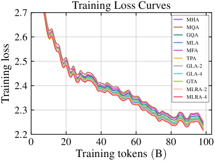
### Visual Description
## Line Chart: Training Loss Curves
### Overview
The chart displays training loss curves for multiple algorithms over 100 training tokens (B). All curves show a downward trend in training loss, starting near 2.7 and converging toward 2.2 by 100 tokens. Lines are closely grouped, with minor fluctuations, suggesting similar performance across algorithms.
### Components/Axes
- **X-axis**: "Training tokens (B)" (0 to 100, linear scale).
- **Y-axis**: "Training loss" (2.2 to 2.7, linear scale).
- **Legend**: Located at the top-right, listing 11 algorithms with color-coded lines:
- MHA (purple)
- MQA (brown)
- GQA (teal)
- MLA (blue)
- MFA (pink)
- TPA (yellow)
- GLA-2 (gray)
- GLA-4 (light blue)
- GTA (green)
- MLRA-2 (orange)
- MLRA-4 (red)
### Detailed Analysis
- **Line Trends**:
- All lines exhibit a consistent downward slope, indicating reduced training loss as tokens increase.
- **MLRA-4 (red)** shows the steepest initial decline, reaching ~2.35 by 100 tokens.
- **GTA (green)** and **MLRA-2 (orange)** exhibit slightly more fluctuation but follow the same general trend.
- **TPA (yellow)** and **GLA-4 (light blue)** remain marginally higher (~2.38–2.40) at 100 tokens.
- **Key Data Points**:
- At 0 tokens: All lines start near 2.7.
- At 50 tokens: Most lines cluster between 2.35–2.40.
- At 100 tokens: Lines converge between 2.25–2.35.
### Key Observations
1. **Convergence**: All algorithms show similar performance by 100 tokens, with losses within ~0.1 of each other.
2. **Early Performance**: MLRA-4 demonstrates the fastest initial improvement, suggesting superior optimization in early training stages.
3. **Stability**: Lines exhibit minor oscillations (e.g., ~2.38–2.42 at 40 tokens), indicating minor instability in loss reduction.
### Interpretation
The chart suggests that all tested algorithms effectively reduce training loss over time, with **MLRA-4** outperforming others in early-stage optimization. The convergence of lines by 100 tokens implies diminishing returns in performance differentiation as training progresses. The minor fluctuations highlight potential sensitivity to hyperparameters or data noise. This analysis could guide algorithm selection for tasks prioritizing rapid initial loss reduction.
</details>
Figure 7: Training loss curves for all models.
<details>
<summary>2603.02188v1/x8.png Details</summary>
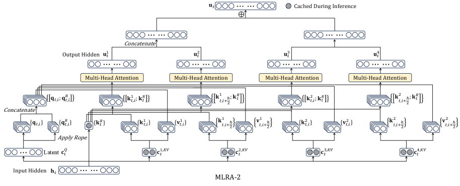
### Visual Description
## Diagram: MLRA-2 Architecture
### Overview
The diagram illustrates the architecture of the MLRA-2 model, a multi-stage processing pipeline for sequence data. It features input/output hidden states, multi-head attention mechanisms, concatenation operations, and cached inference states. The flow progresses from left (input) to right (output), with parallel processing paths and feedback loops.
### Components/Axes
1. **Input/Output States**:
- **Input Hidden**: `h_t` (leftmost node)
- **Output Hidden**: `u_t` (topmost node, cached during inference)
2. **Processing Blocks**:
- **Multi-Head Attention**: Four parallel blocks (labeled `u₁`, `u₂`, `u₃`, `u₄`)
- **Concatenate**: Merges outputs of attention heads
- **Apply Rope**: Positional encoding applied to latent states
3. **Latent States**:
- `c_t`, `c₁,KV`, `c₂,KV`, `c₃,KV`, `c₄,KV` (intermediate cached values)
4. **Key Vectors**:
- `k_t`, `k₁`, `k₂`, `k₃`, `k₄` (query/key vectors for attention)
- `v_t`, `v₁`, `v₂`, `v₃`, `v₄` (value vectors for attention)
5. **Legend**:
- **Cached During Inference**: Striped pattern (applies to `u_t` and latent states)
### Detailed Analysis
- **Input Flow**:
- `h_t` is split into query (`q_t`) and key (`k_t`) vectors.
- Queries and keys are processed through multi-head attention, generating intermediate latent states (`c₁,KV` to `c₄,KV`).
- **Attention Mechanism**:
- Each attention head (`u₁` to `u₄`) computes weighted sums of value vectors (`v₁` to `v₄`).
- Outputs are concatenated and passed through another attention layer to produce `u_t`.
- **Caching**:
- `u_t` and latent states (`c₁,KV` to `c₄,KV`) are marked as cached during inference, suggesting optimization for autoregressive generation.
### Key Observations
1. **Parallel Processing**: Four attention heads operate in parallel, enabling efficient computation.
2. **Positional Encoding**: `Apply Rope` indicates integration of positional information for sequence-aware modeling.
3. **Caching Strategy**: Critical states (`u_t`, `c₁,KV`–`c₄,KV`) are preserved to reduce redundant computation during inference.
4. **Feedback Loops**: Outputs from later stages (`u₃`, `u₄`) feed back into earlier attention heads, suggesting recurrent or hierarchical processing.
### Interpretation
The MLRA-2 architecture prioritizes **efficiency** and **sequence modeling**:
- **Efficiency**: Caching mechanisms (`u_t`, `c₁,KV`–`c₄,KV`) minimize recomputation, critical for long-sequence tasks.
- **Sequence Awareness**: Positional encoding (`Apply Rope`) and attention heads capture dependencies across time steps.
- **Hierarchical Design**: Parallel attention heads and feedback loops suggest a layered approach to feature extraction, balancing local and global context.
This design aligns with transformer-based models but introduces optimizations (e.g., selective caching) for specialized applications like autoregressive text generation or time-series forecasting.
</details>
Figure 8: Illustration of MLRA-2.
<details>
<summary>2603.02188v1/x9.png Details</summary>
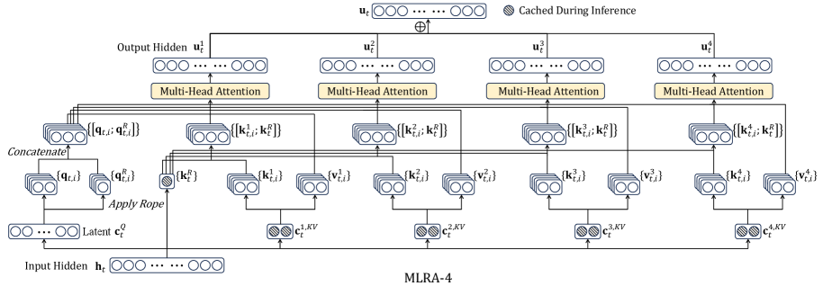
### Visual Description
## Diagram: MLRA-4 Architecture
### Overview
The diagram illustrates the architecture of the MLRA-4 model, a transformer-based system with sequential processing layers. It emphasizes multi-head attention mechanisms, concatenation, positional encoding ("Rope"), and latent representation generation. The flow progresses from input to output through four attention heads, with cached inference steps highlighted.
### Components/Axes
- **Title**: "MLRA-4" (model name) at the bottom center.
- **Legend**: "Cached During Inference" (gray icon) on the right side.
- **Layers**:
- **Input Hidden**: Bottom layer with nodes labeled `h_t` (input sequence).
- **Multi-Head Attention**: Four parallel blocks (labeled 1–4) processing `h_t` into `u1`–`u4`.
- **Concatenate**: Merges outputs from all attention heads.
- **Apply Rope**: Applies positional encoding to concatenated features.
- **Latent cQ**: Outputs compressed latent representations (`c_t^1`–`c_t^4`).
- **Output Hidden**: Top layer with nodes `u1`–`u4` (final outputs).
### Detailed Analysis
1. **Input Hidden (`h_t`)**:
- Represents the initial input sequence (e.g., token embeddings).
- Positioned at the bottom, feeding into all attention heads.
2. **Multi-Head Attention Blocks**:
- Four identical blocks (1–4) process `h_t` into `u1`–`u4`.
- Each block includes key (`k_t^i`), query (`q_t^i`), and value (`v_t^i`) projections.
- Arrows indicate parallel computation paths.
3. **Concatenate**:
- Combines `u1`–`u4` into a single feature vector.
- Positioned centrally, bridging attention heads and subsequent steps.
4. **Apply Rope**:
- Applies rotational positional encoding to concatenated features.
- Outputs `c_t^1`–`c_t^4` (latent representations with positional context).
5. **Output Hidden (`u1`–`u4`)**:
- Final outputs of the attention heads, positioned at the top.
- Connected to the concatenation step via feedback loops (dashed arrows).
### Key Observations
- **Parallel Processing**: Four attention heads enable simultaneous feature extraction.
- **Positional Encoding**: "Rope" step ensures sequence order is preserved in latent representations.
- **Caching**: Gray icons mark cached computations during inference (e.g., `k_t^R`, `v_t^R`).
- **Feedback Loops**: Dashed arrows suggest iterative refinement of attention weights.
### Interpretation
The MLRA-4 architecture resembles a transformer decoder with enhancements for efficiency:
1. **Multi-Head Attention**: Captures diverse contextual relationships in the input sequence.
2. **Latent Compression**: The "Rope" step and `c_t` outputs suggest dimensionality reduction for downstream tasks.
3. **Caching**: Optimizes inference speed by reusing precomputed attention weights (`k_t^R`, `v_t^R`).
4. **Sequential Flow**: Input → Attention → Concatenation → Positional Encoding → Output mirrors standard transformer pipelines but with added optimizations.
This model likely balances accuracy and efficiency, suitable for real-time applications requiring sequential data processing (e.g., NLP, time-series analysis).
</details>
Figure 9: Illustration of MLRA-4.
## Appendix I Related Work
KV Cache Compression.
Recent works (Liu et al., 2023; Anagnostidis et al., 2023; Zhang et al., 2023b; Ge et al., 2024; Xiao et al., 2024; Kim et al., 2024; Zhang et al., 2024b; Nawrot et al., 2024; Tang et al., 2024; Liu et al., 2024b; Dong et al., 2024; Cai et al., 2024; Liu et al., 2024a; Hooper et al., 2024; Sun et al., 2024; Chen et al., 2024a; Jiang et al., 2024; Li et al., 2024; Xiao et al., 2025; Sun et al., 2025; Meng et al., 2025; Tang et al., 2025) don’t introduce new attention mechanisms; instead, they compress the KV cache for pretrained models. Some of these works (Liu et al., 2024b; Hooper et al., 2024) use quantization to store the KV cache in low-bit formats. Some other approaches (Zhang et al., 2023b; Xiao et al., 2024; Li et al., 2024; Xiao et al., 2025) retain important tokens and discard others to compress the KV cache.
Low-Rank Approximation.
Low-rank approximation (Hu et al., 2022; Malladi et al., 2023; Zhang et al., 2023a; Dettmers et al., 2023; Lialin et al., 2024; Zhu et al., 2024; Zeng and Lee, 2024; Chen et al., 2024b; Lin et al., 2025; Wang et al., 2025; Chang et al., 2025) are widely used to compress representations to a low-dimensional space, then up-project to recover full representations. These methods greatly reduce trainable parameters (Hu et al., 2022; Dettmers et al., 2023) during fine-tuning and decrease the number of parameters (Lin et al., 2025; Wang et al., 2025) for pretrained models.
System for Attention.
FlashAttention (Dao et al., 2022; Dao, 2024; Shah et al., 2024) uses tiling and online softmax to minimize reads and writes between high-bandwidth memory and on-chip SRAM, shifting attention from a memory bottleneck to a compute bottleneck. FlashMLA (Jiashi Li, 2025) avoids explicit KV materialization during attention decoding by absorbing the key up-projection matrices into the queries. The following attention computation is similar to MQA with shared KV states. Inspired by classical virtual memory and paging in operating systems, PagedAttention (Kwon et al., 2023) and vLLM use block-level memory management and preemptive request scheduling to reduce fragmentation and redundant duplication.
Linear Attention.
Linear attention (Katharopoulos et al., 2020; Peng et al., 2021; Schlag et al., 2021; Gu et al., 2022; Smith et al., 2023; Sun et al., 2023; Qin et al., 2023; Yang et al., 2024a; Dao and Gu, 2024; Peng et al., 2024; Gu and Dao, 2024; Beck et al., 2024; Zhang et al., 2024a; Yang et al., 2024b; 2025c) reformulates the attention mechanism by substituting the exponential kernel in softmax with a dot product between the query and key vectors. It reduces the memory complexity per decoding step from $O≤ft(n\right)$ for full attention to $O≤ft(1\right)$ .