# Evaluating Pretrained General-Purpose Audio Representations for Music Genre Classification
**Authors**: Kashish Rai, Mrinmoy Bhattacharjee
institutetext: Dept. of Mathematics, Indian Institute of Technology Patna institutetext: Dept. of CSE, Indian Institute of Technology Jammu email: raikashish1002@gmail.com
## Abstract
This study investigates the use of self-supervised learning embeddings, particularly BYOL-A, in conjunction with a deep neural network classifier for Music Genre Classification. Our experiments demonstrate that BYOL-A embeddings outperform other pre-trained models, such as PANNs and VGGish, achieving an accuracy of 81.5% on the GTZAN dataset and 64.3% on FMA-Small. The proposed DNN classifier improved performance by 10-16% over linear classifiers. We explore the effects of contrastive and triplet loss and multitask training with optimized loss weights, achieving the highest accuracy. To address cross-dataset challenges, we combined GTZAN and FMA-Small into a unified 18-class label space for joint training, resulting in slight performance drops on GTZAN but comparable results on FMA-Small. The scripts developed in this work are publicly available. https://github.com/kashishrai12/musicgenre-classification
## 1 Introduction
Music, a universally appealing art form, is often categorized into genres like jazz, pop and others. Music Genre Classification (MGC) helps in efficient music archiving and retrieval. Researchers have used audio feature engineering to create discriminative representations for training classifiers for MGC [9, 11, 8]. Recent studies show that deep audio foundation models, trained on large datasets via Self-Supervised Learning (SSL), are highly effective at generating discriminating feature embeddings for MGC [7, 15, 13, 6, 5]. This work explores the impact of carefully designed classifiers using SSL embeddings for MGC.
Singh et al. [11] compare the effectiveness of standard audio feature representations like Chromagram, Mel-Frequency Cepstral Coefficients (MFCC), and Swaragram [12] with deep learning models like Convolutional Neural Networks (CNN) and Recurrent Neural Networks (RNN) for the MGC task. Their results indicate that Mel-scale features and Swaragram features are the most generic representations across datasets. Other researchers have also utilized music spectrograms as input features for training classifiers for MGC [8]. Ru et al. [9] proposed a multi-modal and multi-label MGC approach by leveraging the inter-genre correlations and the relationship between parallel music and lyrics data.
Recent MGC research has shifted from signal processing-based features to deep SSL embeddings. Zhao et al. [15] introduced the S3T model, trained with a momentum-based contrastive learning approach using the Swin Transformer backbone for MGC and music tagging tasks. Spijkervet et al. [13] developed the CLMR framework, based on SimCLR, for music classification from raw audio waveforms, utilizing data augmentation techniques. Niizumi et al. [7] proposed BYOL-A, an SSL framework for audio, extending BYOL with audio-specific augmentations and a novel encoder. Kong et al. [6] introduced Pretrained Audio Neural Networks (PANNs), large-scale pre-trained convolutional networks for audio classification and MGC tasks. Hershey et al. [5] proposed the VGGish model, a CNN architecture pre-trained on YouTube data and established a baseline for audio embedding extraction in music information retrieval.
Previous work has mainly focused on extracting generalizable SSL embeddings , often using a simple linear layer to map embeddings to target labels of the downstream task. However, limited attention has been given to designing classifier architectures or learning frameworks to improve MGC performance using SSL embeddings. This work explores the impact of carefully designed classifiers trained on SSL embeddings to enhance MGC. The paper is structured as follows. Section 2 presents the methodology for designing a better MGC classifier with SSL embeddings, Section 3 covers experiments and results, and Section 4 concludes the paper.
<details>
<summary>2603.13871v1/sys_diag2.png Details</summary>
### Visual Description
## Flowchart: Audio Genre Classification Pipeline
### Overview
The diagram illustrates a two-stage technical pipeline for audio genre classification. The left section ("BYOL-A Feature Extractor") processes raw audio input through self-supervised feature extraction, while the right section ("DNN Classifier") uses these features for genre prediction via multitask learning. The flow progresses left-to-right through sequential processing stages.
### Components/Axes
**BYOL-A Feature Extractor (Left Section):**
1. Input (blue rectangle)
2. Preprocessing (log-mel spectrogram) (green rectangle)
3. Pre-Norm (light yellow rectangle)
4. Mixup (yellow rectangle)
5. Random Resize Crop (medium yellow rectangle)
6. Random Linear Fader (light yellow rectangle)
7. Post-Norm (white rectangle)
8. 3072-D Embedding (darker yellow rectangle)
**DNN Classifier (Right Section):**
1. Linear Layers (pink rectangle)
2. BatchNorm + ReLU + Dropout (light pink rectangle)
3. Multitask Heads (Cross-Entropy, Contrastive Loss, Triplet Loss) (medium pink rectangle)
4. Genre Prediction (blue rectangle)
**Flow Direction:** All components connected by rightward arrows. Color coding differentiates sections: blue/green for input processing, yellow for augmentation, pink for classification.
### Detailed Analysis
**BYOL-A Feature Extractor:**
- **Preprocessing:** Converts raw audio to log-mel spectrogram representation
- **Normalization:** Pre-Norm and Post-Norm stages suggest batch normalization implementation
- **Augmentation:** Mixup, Random Resize Crop, and Random Linear Fader indicate data augmentation techniques
- **Embedding:** Final 3072-dimensional feature vector output
**DNN Classifier:**
- **Feature Processing:** Linear layers followed by BatchNorm + ReLU + Dropout for regularization
- **Multitask Learning:** Three concurrent loss functions:
- Cross-Entropy (standard classification)
- Contrastive Loss (similarity learning)
- Triplet Loss (embedding space optimization)
- **Output:** Final genre prediction
### Key Observations
1. **Pipeline Structure:** Clear separation between feature extraction (BYOL-A) and classification (DNN)
2. **Augmentation Emphasis:** Three distinct augmentation techniques in feature extraction phase
3. **Multitask Complexity:** Three loss functions operating simultaneously in classification phase
4. **Dimensionality:** 3072-D embedding suggests high-dimensional feature space
### Interpretation
This diagram represents a sophisticated audio classification system combining:
1. **Self-Supervised Learning (BYOL):** The feature extractor uses contrastive learning principles (evidenced by Mixup and Random operations) to learn representations without labeled data
2. **Multitask Learning:** The classifier simultaneously optimizes for three different objectives, potentially improving generalization through shared representations
3. **Architectural Choices:**
- The 3072-D embedding dimension balances capacity and computational efficiency
- BatchNorm + ReLU + Dropout combination suggests careful attention to training stability
- Triplet Loss implementation indicates interest in metric learning for better embedding discrimination
The pipeline demonstrates a modern approach to audio classification that leverages both self-supervised pre-training and multitask fine-tuning, likely resulting in improved performance on genre classification tasks compared to single-task approaches.
</details>
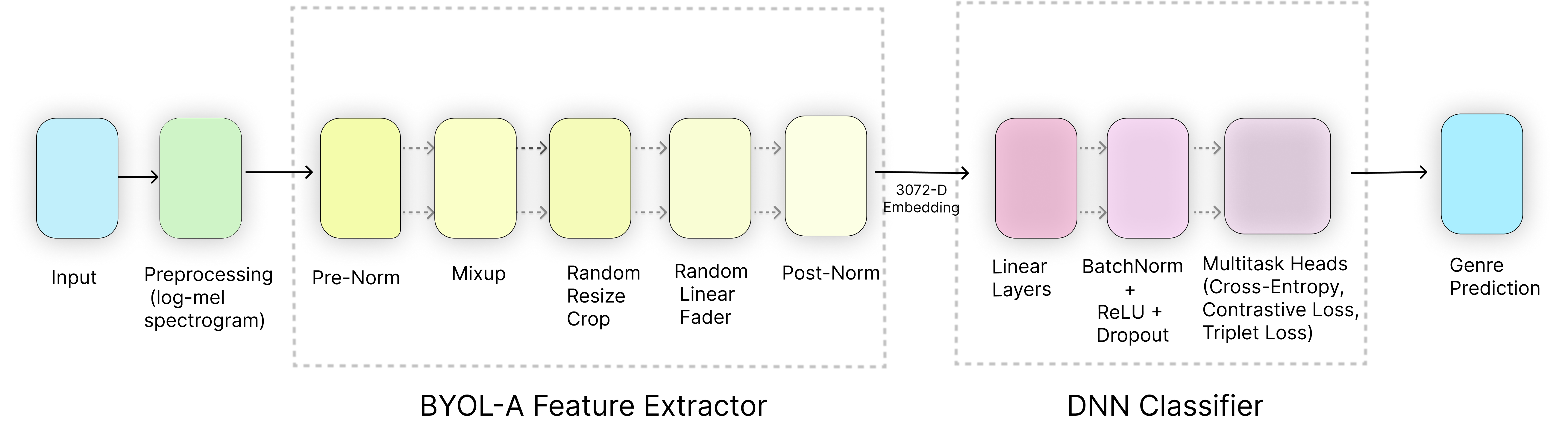
Figure 1: Diagram representing the proposed MGC system. The system consists of SSL embedding extractor followed by an DNN classifier for music genre prediction.
## 2 Methodology
This work uses general-purpose audio SSL models to extract feature embeddings and train carefully designed classifiers to improve MGC performance. A block diagram of the proposed system is illustrated in Fig. 1. The feature extraction approach used in this work is described below.
### 2.1 Feature Extraction
This work compares three different pre-trained SSL models for extracting feature representations, viz., BYOL-A [7], PANNs [6], and VGGish [5]. Each of these models is briefly described next.
In BYOL-A [7], raw audio is converted to log-mel spectrograms and fed into a dual-network architecture with an online and target network. Augmentations like Mixup, Random Resize Crop, and Random Linear Fader are applied to ensure robustness to common audio perturbations. The encoder combines convolutional feature maps and temporal pooling to capture both local and global features. This results in a $3072$ -dimensional embedding for each 30-second audio track, encoding both temporal and spectral characteristics.
We use the CNN14 model from the PANNs framework [6] to extract audio embeddings. Pretrained on the large-scale AudioSet dataset [3], PANNs capture rich acoustic patterns. The input waveform is converted to a log-mel spectrogram and processed by a deep CNN with convolutional blocks and global pooling. The model outputs a $2048$ -dimensional embedding per segment, summarizing spectral and temporal information. The embeddings are averaged over time to form a compact representation for each $30$ s audio clip.
Hershey et al. [5] introduced VGGish, a compact audio feature extractor based on the VGG architecture [10] and pretrained on AudioSet [3]. Audio is resampled to $16$ kHz and converted into $0.96$ s log-mel spectrogram patches, which are processed by a VGG-like network to produce 128-dimensional embeddings. For our experiments, embeddings from a $30$ s audio track are averaged to create a fixed-length feature vector for MGC tasks. The next subsection discusses the classifier training details.
### 2.2 Classifier Training
Our approach centers on designing and training a DNN classifier to map SSL embeddings to music genre labels. The architecture is tailored to utilize the high-dimensional feature space and prevent overfitting. The input layer receives the SSL embedding, followed by hidden layers with linear transformations, Batch Normalization, ReLU activation, and Dropout regularization. These layers progressively reduce dimensions, ensuring effective feature abstraction and regularization. The final architecture was determined empirically.
In the initial experiments for the MGC task, the classifiers are trained using the cross-entropy loss, as defined below.
$$
L_CE=-\frac{1}{N}∑_i=1^Nlog(p_i) \tag{1}
$$
where, $p_i$ is the predicted probability of true class for the $i^th$ sample and $N$ is the number of samples in the batch. To further enhance the discriminative capacity of the learned representations, we explored advanced loss functions, viz., contrastive loss and triplet loss. Some previous works have also explored contrastive loss for the classification of music genres [9, 1, 13]. The contrastive loss is defined as follows [4].
$$
L_CL=\frac{1}{N}∑_i=1^N≤ft\{(1-y_i)·\max≤ft(m-D_w≤ft(z_i^(1),z_i^(2)\right),0\right)^2+y· D_w≤ft(z_i^(1),z_i^(2)\right)^2\right\} \tag{1}
$$
where, $D_w≤ft(z_i^(1),z_i^(2)\right)=√{∑_k=1^n{≤ft(z_i^(1)[k]-z_i^(2)[k]+ε\right)^2}}$ is the Euclidean distance, $ε=1e^-6$ is used for numerical stability, $z_i^(1)$ and $z_i^(2)$ are the model outputs for the $i^th$ input $x_i$ , $y$ is a binary label indicating similar ( $y=0$ ) or dissimilar ( $y=1$ ) pairs, and $m=1.0$ is the loss margin. We have also explored the Triplet loss, which is described below.
$$
L_TL=D_w≤ft(F≤ft(x_i^(a)\right),F≤ft(x_i^(p)\right)\right)-D_w≤ft(F≤ft(x_i^(a)\right),F≤ft(x_i^(n)\right)\right)+ε \tag{3}
$$
where, $F$ is the model that takes the $i^th$ input $x_i$ and produces a $d$ -dimensional output $F≤ft(x_i\right)$ , and $ε$ is the bias term. Superscripts $(a)$ , $(p)$ , and $(n)$ denote the anchor, positive, and negative samples, respectively. These losses were incorporated into the training regime as single-task and multi-task setups alongside the standard cross-entropy loss. The multi-task setup involved multiple output heads, each optimized for a specific loss component, with carefully adjusted weighting parameters. For example, the total loss in the multi-task training, with separate output heads for cross-entropy, contrastive, and triplet losses, is computed as $L=α· L_CE+β· L_CL+≤ft(1-α-β\right)· L_TL$ . Details of the various configurations explored are provided in subsection 3.3.
## 3 Experiments and Results
To evaluate the proposed approach, we conducted experiments to assess the impact of architectural choices, feature extraction methods, and training strategies on MGC performance. Embeddings from BYOL-A [7], PANNs [6], and VGGish [5] were used as input features for the classifier. Two datasets were used for benchmarking: GTZAN [14], consisting of $1000$ half-minute music excerpts labeled in $10$ categories, and the FMA Small subset [2], with $8000$ $30$ s tracks labeled into $8$ genres. A consistent feature extraction pipeline was applied to both datasets, and embeddings from different models were compared. The experiments and results are detailed in the following subsections.
<details>
<summary>2603.13871v1/depth_variation.png Details</summary>
### Visual Description
## Bar Chart: Test Accuracy (%) by Depth Variation
### Overview
The chart compares test accuracy percentages across neural network architectures with varying depths (1 to 4 layers). Accuracy is measured on a y-axis from 70% to 85%, with four distinct bars representing different layer configurations.
### Components/Axes
- **X-axis (Depth Variation)**: Categorical axis labeled "1 Layer," "2 Layers," "3 Layers," and "4 Layers."
- **Y-axis (Test Accuracy %)**: Numerical axis ranging from 70% to 85% in 1% increments.
- **Legend**: Located on the right side of the chart, associating colors with layer configurations:
- Blue: 1 Layer
- Green: 2 Layers
- Red: 3 Layers
- Orange: 4 Layers
- **Bars**: Four vertical bars with explicit percentage labels:
- 1 Layer: 76.0% (blue)
- 2 Layers: 77.0% (green)
- 3 Layers: 78.5% (red)
- 4 Layers: 76.5% (orange)
### Detailed Analysis
- **1 Layer**: Blue bar at 76.0%, the lowest accuracy among all configurations.
- **2 Layers**: Green bar at 77.0%, showing a 1.0% improvement over 1 layer.
- **3 Layers**: Red bar at 78.5%, the highest accuracy, representing a 1.5% increase from 2 layers.
- **4 Layers**: Orange bar at 76.5%, a 2.0% drop from the 3-layer configuration, returning to near 1-layer performance.
### Key Observations
1. **Optimal Depth**: 3-layer networks achieve peak accuracy (78.5%), outperforming all other configurations.
2. **Diminishing Returns**: Adding a fourth layer reduces accuracy by 2.0%, suggesting overfitting or architectural inefficiency.
3. **Color Consistency**: Legend colors (blue, green, red, orange) unambiguously map to their respective layer counts without overlap.
### Interpretation
The data demonstrates a clear non-linear relationship between network depth and test accuracy. While increasing layers from 1 to 3 improves performance, the subsequent drop at 4 layers implies that deeper architectures may introduce complexity without proportional benefits. This pattern aligns with common machine learning principles where optimal model complexity balances bias and variance. The 3-layer configuration represents a Pareto-efficient solution, achieving maximum accuracy with minimal layers. The color-coding enhances interpretability, though the absence of error bars or confidence intervals limits understanding of result reliability.
</details>
<details>
<summary>2603.13871v1/width_variation.png Details</summary>
### Visual Description
## Bar Chart: Test Accuracy vs. Width Variation
### Overview
The image is a bar chart comparing test accuracy (%) across three width variations of a model: 0.5x Nodes, 1.5x Nodes, and 2x Nodes. The y-axis represents test accuracy (%), ranging from 70% to 85%, while the x-axis categorizes the width variations. Each bar is color-coded (blue, green, red) and labeled with its corresponding accuracy percentage.
### Components/Axes
- **X-axis (Width Variation)**:
- Labels: "0.5x Nodes", "1.5x Nodes", "2x Nodes"
- Position: Bottom of the chart, centered under each bar.
- **Y-axis (Test Accuracy %)**:
- Labels: "70", "75", "80", "85" (with dashed gridlines at 75% and 80%).
- Position: Left side of the chart, vertical.
- **Legend**:
- Not explicitly visible in the image. However, the color coding (blue, green, red) is directly tied to the x-axis categories.
- **Bars**:
- Three vertical bars, each representing a width variation.
- Colors:
- 0.5x Nodes: Blue
- 1.5x Nodes: Green
- 2x Nodes: Red
### Detailed Analysis
- **0.5x Nodes**:
- Test Accuracy: 74.5% (blue bar).
- Position: Leftmost bar, slightly below the 75% gridline.
- **1.5x Nodes**:
- Test Accuracy: 76.5% (green bar).
- Position: Middle bar, between 75% and 80% gridlines.
- **2x Nodes**:
- Test Accuracy: 78.5% (red bar).
- Position: Rightmost bar, near the 80% gridline.
### Key Observations
1. **Increasing Accuracy with Width**:
- Test accuracy rises consistently as the number of nodes increases:
- 0.5x → 1.5x: +2.0% (74.5% → 76.5%)
- 1.5x → 2x: +2.0% (76.5% → 78.5%)
2. **Color Coding**:
- The progression from blue (lowest) to red (highest) visually reinforces the trend.
3. **Gridlines**:
- Dashed lines at 75% and 80% help contextualize the accuracy values.
### Interpretation
The data demonstrates a **linear relationship** between model width (number of nodes) and test accuracy. Each incremental increase in nodes (from 0.5x to 2x) correlates with a 2% improvement in accuracy. This suggests that expanding the model's width enhances performance, though the marginal gains appear consistent across the range.
**Notable Insights**:
- The 2x Nodes configuration achieves the highest accuracy (78.5%), indicating that larger models may be more effective for this task.
- The absence of a legend implies that the color coding is directly tied to the x-axis labels, simplifying interpretation.
- The chart does not show diminishing returns, but with only three data points, further analysis would be needed to confirm trends beyond this range.
**Technical Implications**:
- The results could inform decisions about model scaling, balancing computational costs (more nodes) against performance gains.
- The consistent 2% improvement per node increment suggests a predictable relationship, which could be leveraged for resource allocation in training or deployment.
</details>
(a) (b)
<details>
<summary>2603.13871v1/dropout.png Details</summary>
### Visual Description
## Bar Chart: Test Accuracy (%) vs Dropout Rate
### Overview
The chart visualizes the relationship between dropout rates (0.2 to 0.5) and corresponding test accuracy percentages (77.5% to 79.0%). Four vertical bars represent distinct dropout rates, with colors mapped to specific values via a legend. The y-axis ranges from 70% to 85%, with gridlines at 75%, 80%, and 85%.
### Components/Axes
- **X-Axis (Dropout)**: Categorical scale with values 0.2, 0.3, 0.4, 0.5 (left to right).
- **Y-Axis (Test Accuracy %)**: Linear scale from 70% to 85%, with gridlines at 75%, 80%, and 85%.
- **Legend**: Located on the right, associating colors with dropout rates:
- Blue: 0.2
- Green: 0.3
- Red: 0.4
- Orange: 0.5
- **Bars**: Positioned in ascending dropout rate order, with heights proportional to test accuracy.
### Detailed Analysis
1. **Dropout 0.2 (Blue)**: 77.5% accuracy (shortest bar).
2. **Dropout 0.3 (Green)**: 79.0% accuracy (tallest bar).
3. **Dropout 0.4 (Red)**: 78.0% accuracy (second-shortest bar).
4. **Dropout 0.5 (Orange)**: 78.5% accuracy (second-tallest bar).
### Key Observations
- **Peak Accuracy**: Dropout rate 0.3 achieves the highest test accuracy (79.0%).
- **Non-Linear Relationship**: Accuracy increases from 0.2 to 0.3, then decreases at 0.4, followed by a slight recovery at 0.5.
- **Color Consistency**: All bars match the legend’s color assignments without discrepancies.
- **Narrow Range**: All accuracies fall within 77.5%–79.0%, indicating minimal variation across dropout rates.
### Interpretation
The data suggests an optimal dropout rate of **0.3** for maximizing test accuracy. The non-linear trend implies that excessive regularization (e.g., dropout >0.3) may initially reduce performance but could stabilize with further adjustments (e.g., dropout 0.5). The minimal spread in accuracy highlights robustness across tested dropout rates, though 0.3 remains the clear outlier. This pattern aligns with regularization theory, where moderate dropout balances model complexity and generalization.
</details>
<details>
<summary>2603.13871v1/activation_functions.png Details</summary>
### Visual Description
## Bar Chart: Test Accuracy Comparison of Activation Functions
### Overview
The chart compares the test accuracy (%) of four activation functions: ELU, LeakyReLU, ReLU, and Swish. Each bar represents the percentage accuracy, with values labeled on top of the bars. A red dot is positioned above the LeakyReLU bar, indicating an additional data point or anomaly.
### Components/Axes
- **X-axis**: Labeled "Activation Functions," listing four categories: ELU, LeakyReLU, ReLU, and Swish.
- **Y-axis**: Labeled "Test Accuracy (%)" with a scale from 70 to 85, marked at intervals of 5%.
- **Bars**: Four vertical bars, each colored distinctly:
- ELU: Blue (79.0%)
- LeakyReLU: Green (76.5%)
- ReLU: Red (78.0%)
- Swish: Orange (78.0%)
- **Red Dot**: Positioned above the LeakyReLU bar at 77.5%, conflicting with the bar's labeled value of 76.5%.
### Detailed Analysis
- **ELU**: Highest accuracy at 79.0%, represented by a blue bar.
- **LeakyReLU**: Lowest accuracy at 76.5%, shown as a green bar. A red dot at 77.5% is plotted above it, creating ambiguity.
- **ReLU**: Accuracy of 78.0%, depicted in red.
- **Swish**: Matches ReLU at 78.0%, shown in orange.
- **Y-axis Scale**: Ranges from 70% to 85%, with gridlines at 70, 75, 80, and 85.
### Key Observations
1. **ELU outperforms all other activation functions** by 2.5% compared to LeakyReLU and 1.0% compared to ReLU/Swish.
2. **LeakyReLU underperforms** relative to others, with a 2.5% gap from ELU and a 1.5% gap from ReLU/Swish.
3. **Red Dot Discrepancy**: The red dot at 77.5% for LeakyReLU conflicts with the bar's labeled value of 76.5%. This could indicate:
- A data entry error.
- A secondary metric (e.g., validation accuracy) not explicitly labeled.
- A visualization artifact (e.g., misplaced marker).
### Interpretation
The chart suggests that **ELU is the most effective activation function** for the tested model, while **LeakyReLU lags behind**. The near-identical performance of ReLU and Swish implies they are functionally equivalent in this context. The red dot above LeakyReLU introduces uncertainty, as its value (77.5%) does not align with the bar's label (76.5%). This inconsistency warrants further investigation to determine whether it represents a separate data point, a labeling error, or a visualization mistake. The chart emphasizes the importance of activation function selection in optimizing model performance, with ELU emerging as the clear leader.
</details>
(c) (d)
<details>
<summary>2603.13871v1/advanced_techniques.png Details</summary>
### Visual Description
## Bar Chart: BatchNorm Noise Augmentation Test Accuracy Comparison
### Overview
The chart compares test accuracy percentages for three BatchNorm noise augmentation techniques: "BN+Dropout," "Noise Aug. (Epoch)," and "Noise Aug. (Once)." All methods achieve similar performance, with "Noise Aug. (Epoch)" showing marginally higher accuracy.
### Components/Axes
- **X-axis**: Labeled "BatchNorm Noise Augmentation," listing three categories:
1. BN+Dropout (blue)
2. Noise Aug. (Epoch) (green)
3. Noise Aug. (Once) (red)
- **Y-axis**: Labeled "Test Accuracy (%)" with a scale from 70% to 85%, marked in 1% increments.
- **Legend**: Not explicitly visible in the image, but colors are directly mapped to categories in the x-axis labels.
### Detailed Analysis
1. **BN+Dropout (Blue)**:
- Test Accuracy: 81.0%
- Bar height aligns with the 81% mark on the y-axis.
2. **Noise Aug. (Epoch) (Green)**:
- Test Accuracy: 81.5%
- Bar height is the tallest, slightly exceeding 81%.
3. **Noise Aug. (Once) (Red)**:
- Test Accuracy: 81.0%
- Bar height matches BN+Dropout at 81%.
### Key Observations
- **Noise Aug. (Epoch)** achieves the highest test accuracy (81.5%), outperforming the other two methods by 0.5%.
- **BN+Dropout** and **Noise Aug. (Once)** have identical test accuracies (81.0%), suggesting equivalent performance.
- All methods fall within a narrow range (81.0–81.5%), indicating minimal variation in effectiveness.
### Interpretation
The data suggests that applying noise augmentation at the epoch level ("Noise Aug. (Epoch)") yields marginally better results than combining BatchNorm with dropout or applying noise augmentation once. However, the differences are small (≤0.5%), implying that all three techniques are broadly comparable in practical scenarios. The consistency between BN+Dropout and Noise Aug. (Once) might indicate that the timing of noise application (once vs. per epoch) has negligible impact compared to the augmentation method itself. This could guide optimization efforts toward simpler implementations without significant performance trade-offs.
</details>
(e)
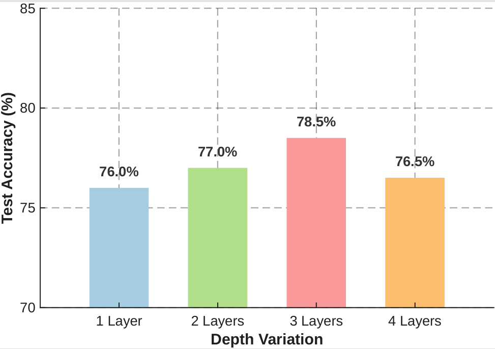
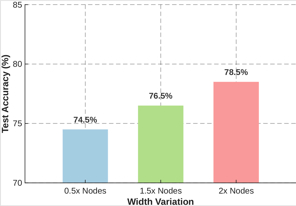
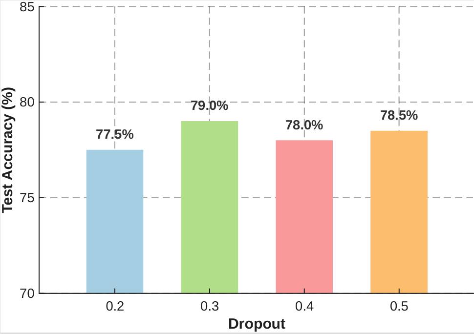
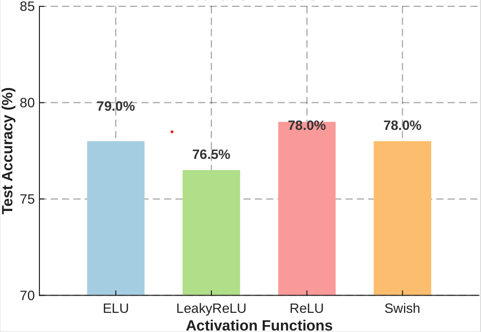
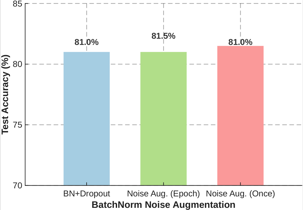
Figure 2: Performance of various model architecture tuning experiments performed on the GTZAN dataset using BYOL-A embeddings as model input feature. The test accuracy (%) for different parameter variations is reported.
### 3.1 Selection of DNN architecture
The impact of hidden layer depth in the DNN classifier was tested with one to four hidden layers (Fig. 2 (a)) using a learning rate of $5e^-4$ and batch size of $64$ . A three-hidden-layer configuration yielded the best performance, with a test accuracy of $78.5\$ . The effect of node count in this configuration ( $128$ , $64$ , and $32$ nodes) was also explored (Fig. 2 (b)), with doubling the node count achieving the best accuracy of $76.5\$ . No other configurations led to significant improvements.
Dropout regularization was tested at various rates (Fig. 2 (c)), with the best performance at a rate of $0.3$ , enhancing generalization. Different activation functions, viz. LeakyReLU, ELU, and Swish were also evaluated (Fig. 2 (d)), with ReLU yielding the highest accuracy of $79\$ . Swish and ELU performed similarly but did not surpass ReLU. After each linear transformation, applying batch normalization was found to stabilize training and improve convergence, achieving a test accuracy of around $81\$ when combined with a dropout rate of $0.3$ .
Table 1: Test Accuracy (%) of using different feature extractors on GTZAN and FMA-Small datasets. Results are reported for our best DNN classifier trained on embeddings from each feature extractor.
| Feature Extractor | GTZAN (%) | FMA-Small (%) |
| --- | --- | --- |
| Niizumi et al. [7] | $70.1$ | $-$ |
| Defferrard et al. [2] | - | $58.0$ |
| Ours + BYOL-A embeddings | $81.5$ | $64.3$ |
| Ours + PANNs embeddings | $77.0$ | $58.0$ |
| Ours + VGGish embeddings | $79.5$ | $58.04$ |
A series of experiments assessed the impact of noise augmentation on model robustness (Fig. 2 (e)). Gaussian noise was added to input embeddings with varied Signal-to-Noise Ratios (SNR) and positions in time. Applying around $20$ dB of Gaussian noise at the start of training yielded the best test accuracy of $81.5\$ . Noise augmentation also reduced the number of epochs for convergence from $50$ to about $35$ and helped prevent overfitting.
### 3.2 Comparison of Feature Extraction Models
A comparison of BYOL-A embeddings with other pre-trained audio models is shown in Table 1. On the GTZAN dataset, BYOL-A achieved $81.5\$ accuracy, outperforming PANNs ( $77\$ ) and VGGish ( $79.5\$ ). BYOL-A also performed better on the FMA-Small dataset with $64.3\$ accuracy. The proposed DNN classifier provided a relative accuracy improvement of $10-16\$ on the GTZAN dataset for all feature extractors and $11\$ on FMA-Small using BYOL-A. These results demonstrate the superior discriminative power of BYOL-A embeddings for MGC and the impact of designing a customized classifier compared to a linear classifier layer.
Table 2: Multitask training results with different loss configurations. Cross-entropy (CE) weights are shown for each classification head, with only one of Contrastive or Triplet used per setup. A ✓ indicates the active loss head, with the weight in brackets.
| | Cross-Entropy ( $α$ ) | Contrastive ( $β$ ) | Triplet ( $≤ft(1-α-β\right)$ ) | Acc (%) | | |
| --- | --- | --- | --- | --- | --- | --- |
| 2 Heads | ✓( $0.5$ ) | - | - | ✓ ( $0.5$ ) | - | $79.0$ |
| ✓( $0.5$ ) | - | - | - | ✓ ( $0.5$ ) | $77.0$ | |
| 3 Heads | ✓( $0.45$ ) | ✓( $0.45$ ) | - | ✓ ( $0.1$ ) | - | $80.0$ |
| ✓( $0.40$ ) | ✓( $0.40$ ) | - | ✓ ( $0.2$ ) | - | $79.5$ | |
| ✓( $0.35$ ) | ✓( $0.35$ ) | - | ✓ ( $0.3$ ) | - | $81.5$ | |
| ✓( $0.30$ ) | ✓( $0.30$ ) | - | ✓ ( $0.4$ ) | - | $77.5$ | |
| ✓( $0.25$ ) | ✓( $0.25$ ) | - | ✓ ( $0.5$ ) | - | $81.0$ | |
| ✓( $0.20$ ) | ✓( $0.20$ ) | - | ✓ ( $0.6$ ) | - | $78.5$ | |
| ✓( $0.15$ ) | ✓( $0.15$ ) | - | ✓ ( $0.7$ ) | - | $79.5$ | |
| ✓( $0.10$ ) | ✓( $0.10$ ) | - | ✓ ( $0.8$ ) | - | $78.0$ | |
| ✓( $0.05$ ) | ✓( $0.05$ ) | - | ✓ ( $0.9$ ) | - | $77.5$ | |
| ✓( $0.07$ ) | ✓( $0.63$ ) | - | ✓ ( $0.3$ ) | - | $80.0$ | |
| ✓( $0.21$ ) | ✓( $0.49$ ) | - | ✓ ( $0.3$ ) | - | $79.5$ | |
| ✓( $0.49$ ) | ✓( $0.21$ ) | - | ✓ ( $0.3$ ) | - | $78.5$ | |
| ✓( $0.63$ ) | ✓( $0.07$ ) | - | ✓ ( $0.3$ ) | - | $81.0$ | |
| ✓( $0.35$ ) | ✓( $0.35$ ) | - | - | ✓ ( $0.3$ ) | $80.0$ | |
| 4 Heads | ✓( $0.23$ ) | ✓( $0.23$ ) | ✓( $0.23$ ) | - | ✓ ( $0.3$ ) | $79.5$ |
### 3.3 Multitask Training
To improve the discriminative power of embeddings, contrastive and triplet loss functions were tested in multitask learning setups with cross-entropy loss. The classifier was extended with multiple output heads, each corresponding to a different loss (e.g., cross-entropy, contrastive, or triplet). Three multitask configurations were explored. First, a $2$ -head setup having contrastive or triplet loss plus an auxiliary cross-entropy head for the anchor sample. Second, a $3$ -head setup has two auxiliary cross-entropy losses for anchor and non-anchor samples besides the main loss function (contrastive or triplet). Finally, a $4$ -head setup was used only for the main loss function as triplet loss with auxiliary cross-entropy heads for anchor, positive, and negative samples. By optimizing a weighted combination of these losses, the model learned representations that were discriminative for genre classification and robust to intra-class variability.
As shown in Table 2, contrastive loss in a $2$ -head setup achieved up to $79\$ accuracy, while triplet loss ranged from $77\$ to $80.5\$ . Multitask training with contrastive and cross-entropy loss achieved the best accuracy of $81.5\$ when loss weights were optimized.
### 3.4 Domain normalization
Table 3: Test Accuracy (%) on GTZAN and FMA-Small using BYOL-A Features
| Training Dataset | GTZAN (%) | FMA-Small (%) |
| --- | --- | --- |
| Niizumi et al. [7] | $70.1$ | - |
| Defferrard et al. [2] | - | $58.0$ |
| Ours (trained on GTZAN) | $81.5$ | - |
| Ours (trained on FMA-Small) | - | $64.3$ |
| Ours (trained on GTZAN + FMA-Small) | $78.0$ | $64.25$ |
The GTZAN and FMA-Small datasets have $10$ and $8$ non-overlapping genres, respectively. Such a scenario makes cross-dataset evaluation difficult. We combined both datasets into a unified label space of $18$ classes for joint training to address this. Using the best DNN architecture with BYOL-A feature extraction, the model was trained to predict one of these $18$ classes. As shown in Table 3, models trained on the combined dataset performed slightly worse on GTZAN but similarly on FMA-Small. While learning MGC on an augmented label space is more challenging, the BYOL-A embeddings with the designed DNN classifier still performed well. Such results highlight the need for domain adaptation to improve generalization.
## 4 Conclusion
This study investigates the effectiveness of SSL embeddings combined with a well-designed DNN classifier for MGC. The approach achieved competitive accuracies on the GTZAN and FMA-Small datasets, with BYOL-A embeddings outperforming PANNs and VGGish in both datasets. Fine-tuning with contrastive and triplet losses provided marginal improvements, while multitask training with contrastive and cross-entropy losses yielded the best accuracy of $81.5\$ . Training on a combined dataset of $18$ genres revealed challenges in domain adaptation. These results emphasize the superior discriminative power of BYOL-A embeddings and the importance of a customized classifier over simple linear layers. Future work will explore embeddings from different SSL model depths and apply domain adaptation techniques to improve cross-dataset performance.
## References
- [1] G. H. Costanzi, L. O. Teixeira, G. Z. Felipe, G. D. Cavalcanti, and Y. M. Costa (2024) Music Genre Classification Using Contrastive Dissimilarity. In Proc. 31st International Conference on Systems, Signals and Image Processing (IWSSIP), pp. 1–8. Cited by: §2.2.
- [2] M. Defferrard, K. Benzi, P. Vandergheynst, and X. Bresson (2017) FMA: A Dataset for Music Analysis. In Proc. 18th International Society for Music Information Retrieval Conference (ISMIR), External Links: 1612.01840 Cited by: Table 1, Table 3, §3.
- [3] J. F. Gemmeke, D. P. W. Ellis, D. Freedman, A. Jansen, W. Lawrence, R. C. Moore, M. Plakal, and M. Ritter (2017) Audio Set: An ontology and human-labeled dataset for audio events. In Proc. IEEE International Conference on Acoustics, Speech and Signal Processing (ICASSP), New Orleans, LA, pp. 776–780. Cited by: §2.1, §2.1.
- [4] R. Hadsell, S. Chopra, and Y. LeCun (2006) Dimensionality reduction by learning an invariant mapping. In Proc. IEEE computer society conference on computer vision and pattern recognition (CVPR’06), Vol. 2, pp. 1735–1742. Cited by: §2.2.
- [5] S. Hershey, S. Chaudhuri, D.P. Ellis, J.F. Gemmeke, A. Jansen, R.C. Moore, M. Plakal, D. Platt, R.A. Saurous, B. Seybold, and M. Slaney (2017) CNN architectures for large-scale audio classification. In Proc. IEEE International Conference on Acoustics, Speech and Signal Processing (ICASSP), pp. 131–135. Cited by: §1, §1, §2.1, §2.1, §3.
- [6] Q. Kong, Y. Cao, T. Iqbal, Y. Wang, W. Wang, and M. D. Plumbley (2020) PANNs: Large-scale pretrained audio neural networks for audio pattern recognition. IEEE/ACM Transactions on Audio, Speech, and Language Processing 28, pp. 2880–2894. Cited by: §1, §1, §2.1, §2.1, §3.
- [7] D. Niizumi, D. Takeuchi, Y. Ohishi, N. Harada, and K. Kashino (2022) BYOL for audio: Exploring pre-trained general-purpose audio representations. IEEE/ACM Transactions on Audio, Speech, and Language Processing 31, pp. 137–151. Cited by: §1, §1, §2.1, §2.1, Table 1, Table 3, §3.
- [8] N. Pelchat and C. M. Gelowitz (2020) Neural Network Music Genre Classification. Canadian Journal of Electrical and Computer Engineering 43 (3), pp. 170–173. Cited by: §1, §1.
- [9] G. Ru, X. Zhang, J. Wang, N. Cheng, and J. Xiao (2023) Improving music genre classification from multi-modal properties of music and genre correlations perspective. In Proc. IEEE International Conference on Acoustics, Speech and Signal Processing (ICASSP), pp. 1–5. Cited by: §1, §1, §2.2.
- [10] K. Simonyan and A. Zisserman (2014) Very deep convolutional networks for large-scale image recognition. arXiv preprint arXiv:1409.1556. Cited by: §2.1.
- [11] Y. Singh and A. Biswas (2022) Robustness of musical features on deep learning models for music genre classification. Expert Systems with Applications 199, pp. 116879. External Links: ISSN 0957-4174 Cited by: §1, §1.
- [12] Y. Singh, R. Kumar, and A. Biswas (2021) Swaragram: Shruti-based chromagram for Indian classical music. In Proc. 25th International Symposium on Frontiers of Research in Speech and Music (FRSM), pp. 109–118. Cited by: §1.
- [13] J. Spijkervet and J. A. Burgoyne (2021-11) Contrastive Learning of Musical Representations. In Proc. 22nd International Society for Music Information Retrieval Conference, pp. 673–681. Cited by: §1, §1, §2.2.
- [14] G. Tzanetakis and P. Cook (2002) Musical genre classification of audio signals. IEEE Transactions on Speech and Audio Processing 10 (5), pp. 293–302. Cited by: §3.
- [15] H. Zhao, C. Zhang, B. Zhu, Z. Ma, and K. Zhang (2022) S3T: Self-Supervised Pre-Training with Swin Transformer For Music Classification. In Proc. IEEE International Conference on Acoustics, Speech and Signal Processing (ICASSP), Vol. , pp. 606–610. Cited by: §1, §1.