# Strategic Delay and Coordination Efficiency in Global Games
**Authors**: Shinkyu Park, Behrouz Touri, and Marcos M. Vasconcelos
> The authors contributed equally to this work and are listed in alphabetical order by their last names.S. Park is with Electrical and Computer Engineering, King Abdullah University of Science and Technology, Thuwal, 23955, Saudi Arabia, B. Touri is with the Department of Industrial and Systems Engineering, University of Illinois Urbana Champaign, Champaign, IL 61820, and M. M. Vasconcelos are with the Department of Electrical and Computer Engineering, FAMU-FSU College of Engineering, Florida State University, Tallahassee, FL 32306, USA. E-mails: {
## Abstract
We investigate a coordination model for a two-stage collective decision-making problem within the framework of global games. The agents observe noisy signals of a shared random variable, referred to as the fundamental, which determines the underlying payoff. Based on these signals, the agents decide whether to participate in a collective action now or to delay. An agent who delays acquires additional information by observing the identities of agents who have chosen to participate in the first stage. This informational advantage, however, comes at the cost of a discounted payoff if coordination ultimately succeeds. Within this decision-making framework, we analyze how the option to delay can enhance collective outcomes. We show that this intertemporal trade-off between information acquisition and payoff reduction can improve coordination and increase the efficiency of collective decision-making.
## I Introduction
Consider a collection of agents sharing a common environment. A task with a random difficulty is introduced, and the agents must coordinate to complete it. However, the task’s difficulty (defined as the number of agents required to complete the task and obtain a positive reward) is imperfectly observed through noisy channels. The agents face a two-stage decision process regarding whether to participate on the task or not. In the first stage, agents may take a risky action and receive an undiscounted payoff. The agents who choose to delay their decision to the second stage receive an additional information signal, observing the set of agents who took the risky action in the first stage, but at the cost of a discounted payoff. From the perspective of a system designer, we seek to determine whether incorporating this second stage is advantageous in equilibrium or not. Addressing this requires evaluating a nontrivial trade-off between the initial noise level in the private signals about the task difficulty, the informational gain achieved by delaying the decision, and the penalty of the discounted payoff. In this paper, we formalize this trade-off to answer this question.
<details>
<summary>2604.05298v1/x1.png Details</summary>
### Visual Description
## Diagram: Two-Stage Signal Processing System
### Overview
The diagram illustrates a two-stage signal processing system involving a central "State" entity that emits signals through two distinct phases. The first stage involves noisy private signals, while the second stage processes these into a noiseless public feedback signal. Arrows indicate directional flow, and colored circles represent discrete actions or events tied to each stage.
---
### Components/Axes
1. **Central Nodes**:
- **State (Θ)**: A central node emitting signals, positioned at the far left.
- **Yᵢ (First Stage)**: A cluster of nodes representing "Private (noisy) signals" in the first stage.
- **S (Second Stage)**: A cluster of nodes representing "Public (noiseless) feedback signal" in the second stage.
2. **Arrows**:
- **Dashed Arrows**: Connect the State to Yᵢ (first stage), indicating noisy signal emission.
- **Solid Arrows**: Connect Yᵢ to S (second stage), showing signal refinement into a noiseless feedback.
3. **Legend**:
- **Blue Circles**: Labeled *Aᵢ⁽¹⁾ = 1*, associated with the first stage (noisy signals).
- **Purple Circles**: Labeled *Aᵢ⁽²⁾ = 1*, associated with the second stage (noiseless feedback).
4. **Text Labels**:
- **First Stage**: "Private (noisy) signals" and "State" (Θ).
- **Second Stage**: "Public (noiseless) feedback signal" and "S".
---
### Detailed Analysis
- **First Stage**:
- The State emits **noisy signals** (Yᵢ) via dashed arrows. These signals are represented by **blue circles** (Aᵢ⁽¹⁾ = 1), indicating discrete events or actions tied to the noisy phase.
- The legend confirms blue corresponds to the first stage, with all blue circles positioned within the light blue region.
- **Second Stage**:
- Noisy signals (Yᵢ) are processed into a **noiseless feedback signal** (S) via solid arrows. This stage is represented by **purple circles** (Aᵢ⁽²⁾ = 1), positioned within the light purple region.
- The legend confirms purple corresponds to the second stage, with all purple circles aligned to the solid arrows.
- **Flow Direction**:
- Signals flow **left to right**: State → Yᵢ (noisy) → S (noiseless).
- The transition from dashed to solid arrows visually emphasizes the refinement of signals from noisy to noiseless.
---
### Key Observations
1. **Signal Transformation**: The system explicitly separates noisy and noiseless processing stages, with the second stage acting as a refinement mechanism.
2. **Action Differentiation**: Blue (Aᵢ⁽¹⁾) and purple (Aᵢ⁽²⁾) circles are spatially isolated, reinforcing the distinction between stages.
3. **Noisy vs. Noiseless**: The absence of noise in the second stage (solid arrows, purple circles) suggests a critical filtering or consensus mechanism.
---
### Interpretation
This diagram models a system where raw, noisy signals (first stage) are transformed into a refined, noiseless output (second stage). The use of distinct colors and arrow styles highlights the progression from uncertainty (noise) to clarity (noiseless feedback). The central "State" acts as the source, while Yᵢ and S represent intermediate and final outputs, respectively. The legend’s spatial placement (top-right) ensures clarity in distinguishing action types. This structure could represent communication protocols, decision-making frameworks, or error-correction systems where noise reduction is critical.
</details>
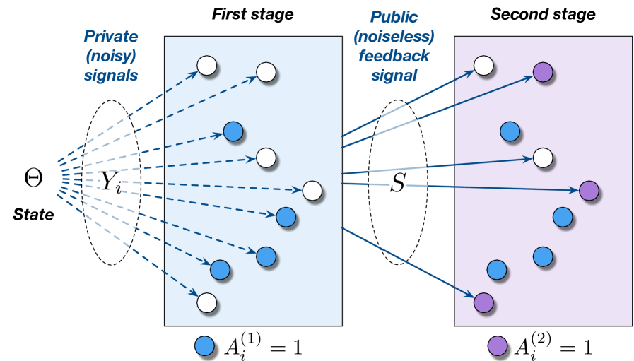
Figure 1: Two-stage global game with public (noiseless) feedback signal. In the first stage, the blue nodes decided to take the risky action, and the white nodes delayed their decision to the second stage. In the second stage the purple nodes decided to take the risky action. The payoff is collected at the end of the game.
The applications of this decision-making framework are broad, spanning engineering [1, 2, 3, 4], economics [5], biology [6], and political science [7]. Specific examples include distributed task allocation in multi-robot systems, speculative currency attacks, bank runs, risky investments, the disclosure of private preferences, microbial infections, and political revolutions [8, 9, 10]. Traditionally, these problems are modeled as global games. This literature was initiated by the seminal work of [11] and further developed and popularized by [12].
The vast majority of this literature focuses on single-stage games. Due to the intrinsic complexity of even the most canonical problem formulations, the analysis of multi-stage global games has remained limited. The work of Dasgupta [13] is among the first to study the option to delay in global games, characterizing coordination regimes in a continuum of agents with binary payoffs. Notably, [13] relies on the assumption of vanishing noise, which serves as an analytical device to ensure desirable properties such as equilibrium uniqueness. In contrast, our approach focuses on the non-vanishing noise regime, although the noise level may still be sufficiently small. In particular, we are interested in scenarios where the noise level could also be manipulated. For example, when an incumbent regime manipulates information to induce instability and hinder coordination within a population. Another arises when a cyber-attacker seeks to disrupt the operations of a swarm robotic system cooperating to fulfill tasks in a smart warehouse.
Building on the setup introduced by [13], we consider a payoff structure that is more closely aligned with the growing engineering and operations research literature on global games. Specifically, the payoff increases linearly with the number of agents taking the risky action and decreases linearly with the task difficulty (i.e., the fundamental). We assume Gaussian prior and noise distributions. In contrast to much of the economics literature, we do not impose degenerate priors or vanishing noise. Instead, we characterize equilibria for given model parameters, allowing for a more direct connection to practical settings.
We begin with a finite population and show that the introduction of a delay option facilitates coordination from the perspective of a mechanism designer. We then analyze the infinite-population limit, where we first identify noise regimes under which the equilibrium in the class of threshold policies is unique, and subsequently derive comparative statics with respect to the discount factor. Finally, by introducing a notion of coordination efficiency, we demonstrate that there exist regimes in which adding a second stage improves equilibrium efficiency and others when it does not.
The remainder of the paper is organized as follows. Section II introduces the model, and Section III studies equilibrium properties in the finite-agent regime. Section IV analyzes the infinite-agent regime, where equilibrium reduces to a single threshold parameter and admits tractable analysis; comparative statics are also presented. Section V introduces coordination efficiency, and Section VI concludes the paper.
## II System Model
Our framework consists of a two-stage stochastic game with partial information. In this section, we introduce the key components of the game and the associated solution concept.
### II-A Agents and actions
Consider a game with a set of agents $[N]{=}}\{1,…,N\}$ . We study both the finite-population case ( $N<∞$ ) and the infinite-population limit ( $N→∞$ ), in which case $[N]=ℕ$ . The decision process unfolds over two stages, indexed by $t∈\{1,2\}$ . At each stage, each agent $i∈[N]$ selects an action from the binary set $A_i{=}}\{0,1\}$ . Following the convention in the global games literature, action $1$ is referred to as the risky, while action $0$ is the safe. The action of the $i$ -th agent at time $t$ is denoted by $A_i^(t)$ .
The agents are allowed to take the risky action at most once across the two stages. This imposes the following constraint $A_i^(1)+A_i^(2)≤ 1, i∈[N]$ on the action sequence. We let $F_i{=}}A_i^(1)+A_i^(2)$ to be the aggregate action of the player over the two stages.
### II-B Information structure and feedback mechanism
The environment is characterized by an underlying fundamental state $Θ$ , drawn from a standard normal distribution, i.e., $Θ∼N(0,1)$ . The agents do not observe $Θ$ directly. Instead, prior to the first decision stage, each agent $i∈[N]$ receives a private signal $Y_i$ , which is a noisy observation of the fundamental. More precisely, we assume
$$
\displaystyle Y_i=Θ+Z_i, i∈[N], \tag{1}
$$
where the idiosyncratic noise $Z_i$ is independently distributed across agents according to $Z_i∼N(0,σ^2)$ .
To capture the dynamics of delayed decision-making, we introduce a public feedback mechanism. At the conclusion of the first stage $t=1$ , all agents observe the proportion of early adopters who chose to take the risky action In this work, our focus will be on symmetric policies and due to the anonymous utility functions, this quantity can be shown to be the sufficient statistics for decision-making. This is illustrated in Fig. ˜ 1. The noiseless public feedback signal is
$$
\displaystyle S{=}}\frac{1}{N}∑_i=1^NA_i^(1). \tag{1}
$$
### II-C Policies, utility, and Bayesian Nash Equilibrium
The agents use policies on their observations to determine their actions. In the first stage, agent $i$ ’s policy relies exclusively on its private signal
$$
\displaystyle A_i^(1)=π_i^(1)(Y_i). \tag{1}
$$
In the second stage, the policy maps the initial private signal and the public feedback on first-stage actions to a final decision
$$
\displaystyle A_i^(2)=π_i^(2)(Y_i,S). \tag{2}
$$
Denote the action of the $i$ -th agent during the game by $A_i{=}}(A_i^(1),A_i^(2))$ , the action profile of all other agents $A_-i=(A_1,…,A_i-1,A_i+1,… A_N)$ , and the fundamental $Θ$ , the utility function of agent $i∈[N]$ is defined as
$$
u_i(A_i,A_-i,Θ)\\
{=}}\big(A_i^(1)+γ A_i^(2)\big)\Bigg(\frac{1}{N}∑_j=1^N\big(A_j^(1)+A_j^(2)\big)-Θ\Bigg), \tag{1}
$$
where $γ∈(0,1)$ denotes the problem’s discount factor.
**Remark 1**
*The utility function is increasing in the aggregate of agents that take the risky action, and decreasing in the fundamental. Therefore, it has strategic complementarity [9]. Moreover, it is linear in the action profile.*
Denote the policy profile of the $i$ -th agent during the game by $π_i=(π_i^(1),π_i^(2))$ and the policy profile $π_-i=(π_1,…,π_i-1,π_i+1,…,π_N)$ adopted by all other agents. Let $U_i$ denote the expected utility of agent $i$ , defined as
$$
\displaystyleU_i\big(π_i,π_-i\big){=}}E\big[u_i(A_i,A_-i,Θ)\big], \tag{6}
$$
where $A_i^(1)=π_i^(1)(Y_i)$ and $A_i^(2)=π_i^(2)(Y_i,S)$ , and $A_j^(1)={π_j}^(1)(Y_j)$ and $A_j^(2)={π_j}^(2)(Y_j,S)$ for ${j≠ i}$ .
**Definition 1**
*A homogeneous policy profile $π^⋆$ is a Bayesian Nash Equilibrium (BNE) if
$$
\displaystyleU_i\big(π^⋆,π_-i^⋆\big) ≥ U_i\big(π,π_-i^⋆\big), i∈[N], \tag{7}
$$
for any admissible policy $π$ , where $π_-i^⋆$ denotes the profile in which all agents other than $i$ adopt the policy $π^⋆$ .*
## III Preliminaries on Finite-Population Model
We focus on policies of the following form.
$$
E≤ft[\frac{1}{N}\Bigg(∑_j≠ i1(Y_j≤\max\{τ^⋆,λ^⋆(S)\})+1\Bigg)-Θ \Bigg| Y_i=y_i\right]\\
≥γE\Bigg[1(Y_i≤λ^⋆(S))≤ft(\frac{1}{N}≤ft(∑_j≠ i1(Y_j≤\max\{τ^⋆,λ^⋆(S)\})\right)+1\right)-Θ\Bigg| Y_i=y_i\Bigg], \tag{8}
$$
**Definition 2**
*The policies of homogeneous threshold type are defined as
$$
\displaystyleπ_i^(1)(Y_i) \displaystyle{=}}1(Y_i≤τ) \displaystyleπ_i^(2)(Y_i,S) \displaystyle{=}}1(Y_i≤λ(S)), \tag{1}
$$
where $1(·)$ denotes the indicator function, $τ$ is the first-stage threshold, and $λ(S)$ is the second-stage threshold, which depends on the first-stage participation $S$ .*
**Lemma 1**
*The BNE policy profile of homogeneous threshold type is characterized by two-stage thresholds $(τ^⋆,λ^⋆)$ , determined as follows The existence of BNE policies of homogeneous threshold type is currently under investigation in a separate paper..*
First stage
Agent $i$ takes the risky action in the first stage, i.e., $Y_i≤τ^⋆$ , if and only if the conditional expected utility from acting in the first stage is no less than that from delaying to the second stage according to (8).
Second stage
Agent $i$ who delayed the decision to the second stage chooses to take the risky action, i.e., $Y_i≤λ^⋆(S)$ , if and only if the conditional expected utility from acting is nonnegative:
$$
\Bigg(1-s-\frac{1}{N}\Bigg)ℙ\Big(Y_j≤λ^⋆(s) \Big| Y_j>τ^⋆, Y_i=y_i, S=s\Big)\\
+\frac{1}{N}+s-E\Big[Θ \Big| Y_i=y_i, S=s\Big]≥ 0, \tag{10}
$$
* Proof:*
Recall that, under the threshold-type policies, the total action taken by agent $i$ across the two stages satisfies $A_i^(1)+A_i^(2)=1(Y_i≤\max\{τ^⋆,λ^⋆(S)\})$ . We begin by analyzing the second stage. Under a homogeneous policy profile characterized by $(τ^⋆,λ^⋆)$ , agent $i$ takes the risky action if and only if the conditional expected utility of acting is greater than or equal to that of not acting, which yields zero utility, leading to (11), where $S$ denotes the set of agents who take action in the first stage, $S=\{ i∈[N]\mid A_i^(1)=1 \}$ . This condition leads to (10).
$$
\frac{1}{N}≤ft(∑_j∉S∪\{i\}E\Big[1(Y_j≤\max\{τ^⋆,λ^⋆(S)\}) \Big| Y_j>τ^⋆,Y_i=y_i,S=s\Big]+1\right)+s-E\Big[Θ \Big| Y_i=y_i,S=s\Big]≥ 0 \tag{11}
$$
Similarly, for the first stage, the agent compares the conditional expected utility of acting immediately with that of delaying the decision to the second stage. Acting immediately yields a higher expected utility if and only if (8) holds. ∎
**Theorem 1**
*The option to delay facilitates participation when $γ∈(0,\bar{γ})$ for some $\bar{γ}>0$ . In particular,
$$
∑_i=1^N1(Y_i≤τ_single^⋆) ≤ ∑_i=1^N1(Y_i≤\max\{τ^⋆,λ^⋆(s)\}) \tag{12}
$$
for all $s=k/N$ , $k∈[N-1]$ .*
* Proof:*
The proof is in Appendix -A. ∎
The above theorem shows that the option to delay can induce a larger number of agents to take the risky action. However, it is not immediate whether this increase in coordination translates into higher expected utility. To characterize when such improvements arise, we henceforth focus on the infinite-population two-stage global game, which admits a tractable characterization of equilibrium behavior. The following proposition establishes a link between the finite- and infinite-population settings.
**Proposition 1**
*Fix a first-stage threshold $τ$ and let ${λ_N^⋆}$ denote the BNE second-stage policy in a population of size $N$ (assuming it exists and it is unique). Suppose the limit $λ^⋆(s)=\lim_N→∞λ_N^⋆(s_N)$ is well-defined, where $s_N$ denotes the realization of the portion of agents acting in the first stage and satisfies $\lim_N→∞s_N=s$ . In the population limit, the limiting policy profile $(τ,λ^⋆)$ is characterized as follows: 1. The second-stage policy satisfies Technically, $(θ,τ,σ,s)$ can be such that the inequality is exact. In that case, the lower limit and the upper limit to $s$ is not the same. However, this situation happens with probability zero.:
$$
\displaystyle\textstyleλ^⋆(s)=\begin{cases}+∞,&if θ=τ-σΦ^-1(s)≤ 1\\
-∞,&otherwise,\end{cases} \tag{13}
$$
where $θ$ denotes the realization of the fundamental $Θ$ .
1. In equilibrium, agent $i$ chooses to take the risky action in the first stage, i.e., $A_i^(1)=1$ , if and only if
$$
E\Big[F(Θ,S)-Θ\mid Y_i=y_i\Big]\\
≥γ E\Big[1(Θ≤ 1) \big(F(Θ,S)-Θ\big)\mid Y_i=y_i\Big], \tag{14}
$$
where
$$
F(Θ,S){=}}Φ≤ft(\frac{\max\{τ,λ^⋆(S)\}-Θ}{σ}\right). \tag{15}
$$*
* Proof:*
The proof is in Appendix -B. ∎
## IV Infinite-Population Model
The equilibrium analysis becomes significantly more tractable in the limit of a large number of agents.
### IV-A First-stage threshold policy
We assume that the agents utilize a homogeneous threshold policy in the first stage. That is, agent $i$ takes the risky action early if and only if their private signal $Y_i$ is below a common critical threshold $τ$ , i.e., $A_i^(1)=1(Y_i≤τ).$
Conditioned on the realization of the fundamental state $Θ=θ$ , the fraction of agents who take the risky action in the first stage is given by
$$
s=\lim_N→∞\frac{1}{N}∑_i=1^N1(Z_i≤τ-θ)\overset{(a)}{=}ℙ\big(Z_i≤τ-θ\big), \tag{16}
$$
where $Z_i∼N(0,σ^2)$ and $(a)$ follows from the strong law of large numbers for exchangeable processes (see e.g. Example 1, Chapter 7.3., [14]). Therefore, under the first-stage threshold policy, the realized variable $S=s$ corresponds to $s=Φ≤ft(\frac{τ-θ}{σ}\right)$ , where $Φ(·)$ denotes the CDF of the standard Gaussian distribution.
Since at the end of the first stage, each agent who did not take the risky action observes the fraction of agents who acted in the first stage, and since, the standard normal CDF $Φ(·)$ is strictly increasing and continuous, it is invertible, allowing to recover the fundamental $θ$ perfectly. Consequently, using this information, each such agent can compute
$$
τ-σΦ^-1(s)=θ. \tag{17}
$$
In the infinite-population regime, this implies that all agents who delay taking the risky action observe the true realization $Θ=θ$ prior to making their second-stage decision.
**Remark 2**
*The exact recovery of the fundamental state by the remaining agents arises from signaling through infinitely many independent binary channels. While each individual agent’s action is based on a noisy private signal, aggregating these actions over an infinite population conveys an unbounded amount of information In the sense of Shannon’s Information Theory [15]. from the first stage to the second. As a result, the continuous parameter $θ$ can be recovered perfectly. This mechanism does not arise in the finite-population setting.*
Because the fundamental is perfectly revealed, the second-stage policy for any agent who has not yet taken the risky action reduces to a deterministic mapping from $θ$ to an action. Consequently, the initial noisy private signal $Y_i$ becomes irrelevant for the remaining decision. This is analogous to sequential social learning, where private signals can be disregarded without loss of optimality once a sufficient number of prior actions has been observed [16, 17]. Henceforth, we denote the total fraction of the population taking the risky action across both stages by $F(θ)$ .
### IV-B Optimal second-stage policy
In the second stage, the fundamental state $Θ=θ$ is perfectly revealed to all agents. The mass of agents who already committed to the risky action in the first stage is given by
$$
F^(1)(θ)=\lim_N→∞\frac{1}{N}∑_i=1^NA_i^(1)=Φ≤ft(\frac{τ-θ}{σ}\right). \tag{1}
$$
The remaining agents, which have a total mass of $1-F^(1)(θ)$ , now play a perfect-information coordination game.
If an agent takes the risky action in the second stage, their payoff is $γ\big(F(θ)-θ\big)$ . Because the state is known, we can identify three distinct strategic regions based on $θ$ :
#### IV-B 1 Upper Dominance Region ( $θ≥ 1$ )
Even if all remaining agents take the risky action, the maximum possible aggregate action is $F(θ)=1$ . The payoff would be $γ(1-θ)≤ 0$ . The risky action is strictly dominated, so the remaining agents take the safe action: $A_i^(2)=0$ .
#### IV-B 2 Lower Dominance Region ( $θ<F^(1)(θ)=s$ )
The payoff is strictly positive even if no additional agents take the risky action, because the first-stage alone guarantees $F^(1)(θ)-θ>0$ . The risky action is strictly dominant, and all remaining agents take the risky action: $A_i^(2)=1$ .
#### IV-B 3 Multiplicity Region ( $s=F^(1)(θ)≤θ<1$ )
The remaining agents play a pure coordination game. If they all take the risky action, the total active population becomes $F(θ)=F^(1)(θ)+F^(2)(θ)=1$ , yielding a positive payoff $γ\big(1-θ\big)>0$ . If all other agents take the safe action, the total active population remains $F^(1)(θ)$ , yielding a negative payoff $γ(F^(1)\big(θ)-θ\big)≤ 0$ . We assume agents coordinate on the Pareto-dominant equilibrium An equilibrium is considered Pareto dominant if there exists no other equilibrium profile that yields a strictly higher expected payoff for at least one agent without decreasing the payoff of any other agent. where the coordination succeeds. Thus, all remaining agents take the risky action: $A_i^(2)=1$ .
Combining these regions, the optimal second-stage policy for the agents who chose delay is an indicator function of $s$
$$
\displaystyle\textstyle{π_i^⋆}^(2)(s)=1(s≥Φ≤ft(\frac{τ-1}{σ}\right)), i∈[N]. \tag{2}
$$
As a result of using ${π_i^⋆}^(2)(s)$ , the total ex-post aggregate action becomes
$$
\displaystyle\textstyle F(θ)=\begin{cases}1,&if θ≤ 1\\
Φ≤ft(\frac{τ-θ}{σ}\right),&if θ>1.\end{cases} \tag{20}
$$
Note that this is consistent with Proposition 1.
### IV-C Equilibrium condition
We now use backward induction to evaluate the optimal first-stage decision. An agent $i$ observing a private signal $Y_i=y$ must weigh the expected utility of taking the risky action in the first stage against the expected utility of delaying the decision. Define the function
$$
\displaystyleΔ(y){=}}E\Big[(1-γ1(Θ<1)\big)\big(F(Θ)-Θ\big)\mid Y_i=y\Big]. \tag{21}
$$
Note that this expression is the utility difference between taking the risky action in the first stage and the second stage, given the information available at the first stage. As discussed in Proposition 1, for the proposed threshold $τ^⋆$ to constitute a BNE policy profile, an agent must be indifferent between taking the risky action in the first stage and delaying the decision to the second stage. This yields the indifference condition $Δ(τ^⋆)=0$ .
To establish the existence of an equilibrium threshold policy, we proceed as follows. First, we notice that $Δ(τ)>0$ as $τ→-∞$ and $Δ(τ)<0$ as $τ→+∞$ . By continuity of $Δ(τ)$ , there must exist at least one value $τ^⋆$ such that $Δ(τ^⋆)=0$ . However, uniqueness cannot be guaranteed unless we impose a condition on the noise variance.
**Theorem 2**
*In the infinite population regime, suppose that noise variance satisfies ${σ^2<2π}$ , then $Δ(τ)$ in (21) is strictly decreasing function of $τ$ . As a result, there exists a unique threshold $τ^⋆$ that characterizes the BNE, i.e., $Δ(τ^⋆)=0$ .*
* Proof:*
Per the discussion above, a (homogeneous) BNE for the infinite population game would be the pair ${\big(1(Y_i≤τ^⋆),1(Θ≤ 1)\big)}$ for the two stage actions, where the threshold $τ^⋆$ satisfies $Δ(τ^⋆)=0$ . Note that
$$
α=\frac{1}{1+σ^2}, Θ\mid Y=τ∼N(ατ,ασ^2). \tag{22}
$$
In other words, $Θ_τ{=}}(Θ\mid Y=τ)$ can be written as
$$
Θ_τ=ατ+σ√{α} Z, Z∼N(0,1). \tag{23}
$$
Note that $Z$ ’s distribution is independent of $τ$ . Define
$$
g(τ,θ){=}}\begin{cases}(1-γ)(1-θ),&θ≤ 1,\\[4.0pt]
Φ≤ft(\dfrac{τ-θ}{σ}\right)-θ,&θ>1.\end{cases} \tag{24}
$$
Then, $Δ(τ)=E\bigl[g(τ,Θ_τ)\bigr].$ For almost every $Z$ , differentiating with respect to $τ$ gives
$$
\frac{d}{dτ}g(τ,Θ_τ)=-α(1-γ) \tag{25}
$$
for $Θ_τ<1$ , and for $Θ_τ>1$ ,
$$
\frac{d}{dτ}g(τ,Θ_τ)=\frac{1}{σ}φ≤ft(\frac{τ-Θ_τ}{σ}\right)+α≤ft(-1-\frac{1}{σ}φ\bigg(\frac{τ-Θ_τ}{σ}\right)\bigg). \tag{26}
$$
Since $1-α=ασ^2$ , this simplifies to
$$
\frac{d}{dτ}g(τ,Θ_τ)=\begin{cases}-α(1-γ),&Θ_τ<1,\\[6.0pt]
α≤ft(σφ≤ft(\dfrac{τ-Θ_τ}{σ}\right)-1\right),&Θ_τ>1.\end{cases} \tag{27}
$$
Note that $-α(1-γ)<0$ , and using $φ(x)≤φ(0)=1/√{2π}$ , we obtain
$$
α≤ft(\frac{σ}{√{2π}}-1\right)<0 whenever σ<√{2π}. \tag{28}
$$
Hence, letting $γ=\max≤ft(-(1-γ), \frac{σ}{√{2π}}-1\right)<0$ , we have
$$
Δ^\prime(τ)=E≤ft[\frac{d}{dτ}g(τ,Θ_τ)\right]≤γ<0. \tag{29}
$$
Since $Δ^\prime(τ)≤γ$ , it follows that $Δ(τ)→-∞$ as $τ→+∞$ and $Δ(τ)→+∞$ as $τ→-∞$ . Hence, by continuity of $Δ(τ)$ , it has a root $τ=τ^⋆$ , which is unique by strict monotonicity. ∎
One of the implications of the above result is that the optimal threshold $τ^⋆$ is a decreasing function of the discount factor $γ$ , which is a natural condition to appear: when $γ$ is small, the agents have more incentive to act on the first stage.
**Proposition 2**
*If $σ^2<2π$ , the equilibrium threshold $τ^⋆$ for taking a risky action on the first stage, is strictly decreasing in the discount factor $γ$ . Therefore, an increase in the discount factor strictly reduces the fraction of agents taking the risky action on the first-stage for any given realization of the fundamental $Θ=θ$ .*
* Proof:*
The equilibrium threshold $τ^⋆$ is uniquely defined by the indifference condition $Δ(τ^⋆;γ,σ)=0$ . By the Implicit Function Theorem, the derivative of the threshold with respect to $γ$ is given by
$$
\frac{dτ^⋆}{dγ}=-\frac{\frac{∂Δ}{∂γ}}{\frac{∂Δ}{∂τ}}. \tag{30}
$$
From the monotonicity established in the proof of Theorem 2, we know that if $σ^2<2π$ , then $\frac{∂Δ}{∂τ}(τ)<0$ . It remains to analyze the partial derivative of $Δ$ with respect to $γ$ . Notice that $γ$ only affects the agent’s payoff when $θ<1$ , where the net payoff of taking a risky action in the first stage versus delaying is $(1-γ)(1-θ)$ . Differentiating $Δ$ with respect to $γ$ gives
$$
\frac{∂Δ}{∂γ}=-∫_-∞^1(1-θ)f(θ\mid Y=τ^⋆) dθ<0, \tag{31}
$$
where the inequality holds since $θ<1$ . From (30), we obtain $\frac{dτ^⋆}{dγ}<0$ . Since the fraction of agents taking the risky action on the first-stage given $Θ=θ$ is $ℙ(Y≤τ^⋆\midΘ=θ)=Φ≤ft(\frac{τ^⋆-θ}{σ}\right)$ , which is strictly increasing in $τ^⋆$ , an increase in $γ$ strictly reduces this probability for any given $θ$ . ∎
## V Coordination Efficiency
To compare the efficiency of the system under two stages vs. single stage homogeneous threshold policies, we consider a metric based on the aggregate expected payoff (i.e., welfare) of all agents. The larger this collective payoff, the more efficient the agents are in terms of coordinating their actions towards performing a task with difficulty $θ$ .
Recall that under a first-stage threshold policy with parameter $τ$ , the first-stage adoption rate as a function of the fundamental $θ$ is given by $F^(1)(θ)=Φ≤ft(\frac{τ-θ}{σ}\right)$ . Under Pareto-dominant equilibrium selection in the second stage, where agents observe $θ$ perfectly through the public signal $s$ , all remaining agents take the risky action if and only if $θ≤ 1$ . This yields a second-stage adoption rate of $\bigl(1-F^(1)(θ)\bigr) 1(θ≤ 1)$ .
To quantify the efficiency of coordination under $τ$ , we define the welfare as
$$
W_two-stage(τ,σ,γ){=}}∫_1^∞\underbrace{F^(1)(θ)\bigl(F^(1)(θ)-θ\bigr)}_aggregate payoff when $θ>1$ φ(θ) dθ\\
+∫_-∞^1\underbrace{\Big[F^(1)(θ)+γ\big(1-F^(1)(θ)\big)\Big](1-θ)}_aggregate payoff when $θ≤ 1$ φ(θ) dθ, \tag{1}
$$
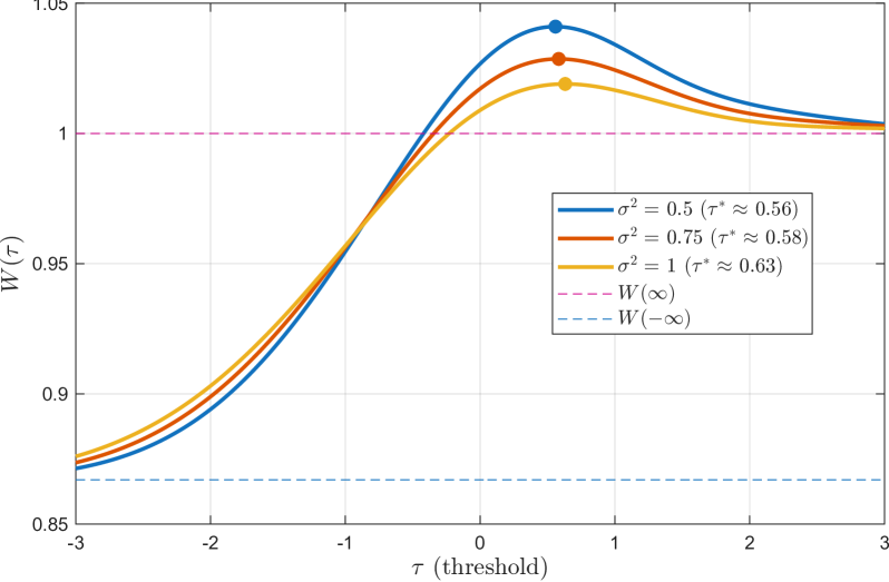
where $φ$ denotes the standard Gaussian density. Figure 2 illustrates the welfare of the two-stage global game as a function of the threshold $τ$ .
<details>
<summary>2604.05298v1/x2.png Details</summary>
### Visual Description
## Line Graph: W(τ) vs. τ (Threshold)
### Overview
The graph depicts the function \( W(\tau) \) as a function of the threshold parameter \( \tau \), with multiple curves representing different variance values (\( \sigma^2 \)). Key features include:
- A horizontal pink dashed line at \( W = 1 \) (labeled \( W(\infty) \)).
- A horizontal blue dashed line at \( W = 0.85 \) (labeled \( W(-\infty) \)).
- Four solid lines for \( \sigma^2 = 0.5, 0.75, 1 \), and their corresponding peak thresholds (\( \tau^* \approx 0.56, 0.58, 0.63 \)).
### Components/Axes
- **X-axis (τ)**: Labeled "τ (threshold)", ranging from -3 to 3.
- **Y-axis (W(τ))**: Labeled "W(τ)", ranging from 0.85 to 1.05.
- **Legend**: Located in the top-right corner, with:
- Blue line: \( \sigma^2 = 0.5 \) (\( \tau^* \approx 0.56 \)).
- Orange line: \( \sigma^2 = 0.75 \) (\( \tau^* \approx 0.58 \)).
- Yellow line: \( \sigma^2 = 1 \) (\( \tau^* \approx 0.63 \)).
- Pink dashed line: \( W(\infty) \).
- Blue dashed line: \( W(-\infty) \).
### Detailed Analysis
1. **Trends**:
- All curves rise from \( W(-\infty) = 0.85 \) (blue dashed line) as \( \tau \) increases.
- Each curve peaks at a specific \( \tau^* \), then declines toward \( W(\infty) = 1 \) (pink dashed line).
- The peak \( \tau^* \) values increase with \( \sigma^2 \): \( 0.56 \) (blue) < \( 0.58 \) (orange) < \( 0.63 \) (yellow).
- The yellow curve (\( \sigma^2 = 1 \)) has the lowest peak \( \tau^* \), while the blue curve (\( \sigma^2 = 0.5 \)) has the highest.
2. **Data Points**:
- At \( \tau = 0 \), all curves are near \( W = 0.9 \).
- At \( \tau = 1 \), the blue curve (\( \sigma^2 = 0.5 \)) reaches its peak (\( W \approx 1.04 \)).
- At \( \tau = 2 \), all curves converge toward \( W = 1 \).
### Key Observations
- **Peak Behavior**: Higher \( \sigma^2 \) values correspond to lower peak thresholds (\( \tau^* \)), suggesting a trade-off between variance and optimal threshold.
- **Convergence**: All curves asymptotically approach \( W(\infty) = 1 \), indicating a universal upper bound.
- **Asymptotic Bound**: \( W(-\infty) = 0.85 \) acts as a lower bound for all \( \sigma^2 \).
### Interpretation
The graph illustrates how \( W(\tau) \) balances variance (\( \sigma^2 \)) and threshold (\( \tau \)) to achieve a maximum value. The peak \( \tau^* \) represents the optimal threshold for each \( \sigma^2 \), where \( W(\tau) \) is maximized. The convergence to \( W(\infty) = 1 \) implies that increasing \( \tau \) beyond the peak yields diminishing returns, while \( W(-\infty) = 0.85 \) sets a baseline performance limit. This could reflect phenomena like signal detection efficiency, where higher noise (\( \sigma^2 \)) requires lower thresholds to maintain performance, but excessive thresholds risk overshooting the optimal point.
</details>
Figure 2: Per agent welfare for a two-stage global game with $γ=0.8$ .
To assess whether the option to delay is beneficial or detrimental in equilibrium, we compare the welfare of the two-stage global game against that of the single-stage global game. The welfare for the single-stage game is given by
$$
\displaystyle W_single-stage(τ,σ){=}}∫_-∞^∞F^(1)(θ)\big(F^(1)\big(θ)-θ\big)φ(θ) dθ. \tag{1}
$$
For the single-stage global game, the indifference condition that determines the BNE threshold is given by [10]:
$$
\displaystyleE\Big[F^(1)(Θ)-Θ\mid Y_i=τ^⋆\Big]=0. \tag{1}
$$
Let $τ_single^⋆(σ)$ denote the BNE threshold of the single-stage global game and $τ^⋆(σ,γ)$ the BNE threshold of the two-stage global game. The value of the second stage is defined as
$$
V(σ,γ){=}}W_two-stage\bigl(τ^⋆(σ,γ), σ, γ\bigr)\\
-W_single-stage\bigl(τ_single^⋆(σ), σ\bigr), \tag{35}
$$
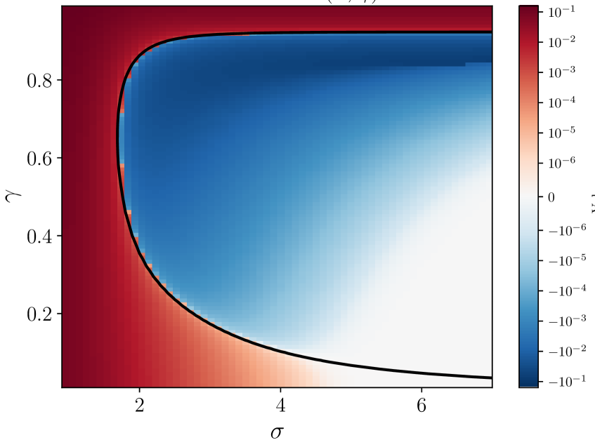
where each welfare is evaluated at the respective equilibrium threshold of its own game. When $V(σ,γ)>0$ , the two-stage game achieves more welfare than the single-stage game: the safety net provided by the noiseless second stage more than compensates for the strategic delay it induces. When $V(σ,γ)<0$ , the opposite holds: more agents tend to postpone their decisions to a costly second stage, and the resulting expected coordination loss exceeds the benefit of taking the risky action.
<details>
<summary>2604.05298v1/x3.png Details</summary>
### Visual Description
## Heatmap: Parameter Space Analysis
### Overview
The image depicts a two-dimensional heatmap visualizing a parameter space defined by variables γ (vertical axis) and σ (horizontal axis). The color gradient transitions from red (positive values) to blue (negative values), with a black boundary curve separating distinct regions. A logarithmic color scale on the right quantifies the magnitude of the values.
### Components/Axes
- **Vertical Axis (γ)**: Labeled with values 0.2, 0.4, 0.6, 0.8, increasing upward.
- **Horizontal Axis (σ)**: Labeled with values 2, 4, 6, increasing rightward.
- **Color Scale**:
- Red (10⁻¹ to 10⁻³) → Orange (10⁻⁴) → Yellow (10⁻⁵) → White (0) → Blue (-10⁻⁵ to -10⁻¹).
- Positioned on the right, vertically aligned.
- **Boundary Curve**: A smooth, concave black curve separating red (positive) and blue (negative) regions. It originates near (σ=2, γ=0.2) and curves upward to intersect the γ-axis near γ=0.8.
### Detailed Analysis
1. **Red Region (Positive Values)**:
- Dominates the lower-left quadrant (σ < 4, γ < 0.6).
- Intensity decreases from dark red (10⁻¹) near σ=2, γ=0.2 to lighter red/orange (10⁻³–10⁻⁴) as σ and γ increase.
- Gradual transition to white near the boundary curve.
2. **Blue Region (Negative Values)**:
- Occupies the upper-right quadrant (σ > 4, γ > 0.6).
- Intensity increases from light blue (-10⁻⁵) near the curve to dark blue (-10⁻¹) at σ=6, γ=0.8.
- Sharp contrast with the red region, indicating a sign change across the boundary.
3. **Boundary Curve**:
- Separates positive (red) and negative (blue) regions.
- Follows a concave shape, suggesting a nonlinear relationship between γ and σ.
- Positioned closer to the σ-axis at lower γ values and shifts upward as σ increases.
### Key Observations
- **Threshold Behavior**: The black curve acts as a decision boundary, demarcating regions of opposing signs.
- **Magnitude Gradient**: Values transition smoothly from extreme magnitudes (10⁻¹) to near-zero (white) near the boundary.
- **Asymmetry**: The red region is more concentrated in the lower σ/γ range, while the blue region dominates higher σ/γ values.
### Interpretation
The heatmap likely represents a function \( f(\gamma, \sigma) \) with critical behavior at the black boundary curve. The red and blue regions suggest opposing phenomena (e.g., stability vs. instability, activation vs. suppression) depending on parameter combinations. The logarithmic scale emphasizes sensitivity to small changes in magnitude, particularly near the boundary. The concave curve implies a nonlinear interaction between γ and σ, potentially indicating a phase transition or bifurcation in the modeled system. The asymmetry in region distribution highlights that higher σ values disproportionately influence the sign change, while γ modulates the transition's steepness.
</details>
Figure 3: Illustration of the function $V(σ,γ)$ defined in (35). The red region indicates the parameter regime $(σ,γ)$ in which the option to delay is beneficial, whereas the blue region corresponds to regimes in which it is detrimental.
### V-A When does the option to delay improve efficiency?
Figure 3 illustrates the regions in which the option to delay is beneficial. Interestingly, the option to delay can also be detrimental. The following theorem formalizes this observation.
**Theorem 3**
*Consider a two-stage global game with infinitely many agents, noisy signals with variance $σ^2$ and discount factor $γ∈(0,1)$ . The following hold
1. For any given noise level $σ>0$ , there exists $\bar{γ}_σ>0$ such that welfare improves for $γ∈(0,\bar{γ}_σ)$ .
1. For any fixed discount factor $γ∈(0,1)$ , there exists $\bar{σ}_γ>0$ such that welfare improves for ${σ∈(0,\bar{σ}_γ)}$ .*
* Proof:*
The proof is in Appendix -C. ∎
**Remark 3**
*An important observation is that the equilibrium threshold $τ^⋆(σ,γ)$ does not, in general, maximize welfare in the two-stage game, i.e.,
$$
W_two-stage\big(τ^⋆(σ,γ),σ,γ\big)<\max_τ∈ℝW_two-stage(τ,σ,γ). \tag{36}
$$
As a result, it may occur that
$$
\textstyle W_two-stage\big(τ^⋆(σ,γ),σ,γ\big)<W_single-stage(τ_single^⋆(σ),σ)\\
<\max_τ∈ℝW_two-stage(τ,σ,γ), \tag{37}
$$
which shows there is a gap between equilibrium and welfare-optimal coordination.*
## VI Conclusions and future work
This work considers a sequential stochastic coordination game with imperfect observations among $N$ agents. Within the class of homogeneous threshold policies, we provided several preliminary results that showed that adding the option to delay taking a risky action and reducing an agent’s payoff may be beneficial. When the system has a finite number of agents, we have shown that adding a second stage increases the probability an agent will take the risky action in the first stage in equilibrium. When the number of agents is asymptotically large, we show there exist regions of the $(γ,σ)$ parameter space where having a second stage is strictly better than not having one. Therefore, the feedback mechanism constitutes an important tool for improving coordination. Future work on this topic includes the characterization of information theoretic limits, learning algorithms, and the impact of social network structure on coordination.
## References
- [1] V. Krishnamurthy, “Decentralized spectrum access amongst cognitive radios—an interacting multivariate global game-theoretic approach,” IEEE Transactions on Signal Processing, vol. 57, no. 10, pp. 3999–4013, 2009.
- [2] A. Kanakia, B. Touri, and N. Correll, “Modeling multi-robot task allocation with limited information as global game,” Swarm Intelligence, vol. 10, no. 2, pp. 147–160, 2016.
- [3] L. E. Beaver, “Multi-robot task allocation using global games with negative feedback: the colony maintenance problem,” in Proceedings of the AAAI Conference on Artificial Intelligence, vol. 39, pp. 13597–13604, 2025.
- [4] Y. Wei and M. M. Vasconcelos, “Strategic multi-task coordination over regular networks of robots with limited computation and communication capabilities,” in 57th Annual Conference on Information Sciences and Systems (CISS), pp. 1–6, 2023.
- [5] Y. Jin, Z. Zhou, and A. Brandenburger, “Coordination via delay: Theory and experiment,” Games and Economic Behavior, vol. 137, pp. 23–49, 2023.
- [6] M. M. Vasconcelos and B. Touri, “Multi-agent coordination under poisson observations: A global game approach,” (submitted to) IEEE Transactions on Automatic Control - arXiv:2507.00424, 2025.
- [7] G.-M. Angeletos, C. Hellwig, and A. Pavan, “Dynamic global games of regime change: Learning, multiplicity, and the timing of attacks,” Econometrica, vol. 75, pp. 711–756, May 2007.
- [8] H. Mahdavifar, A. Beirami, B. Touri, and J. S. Shamma, “Global games with noisy information sharing,” IEEE Transactions on Signal and Information Processing over Networks, vol. 4, no. 3, pp. 497–509, 2017.
- [9] M. A. Dahleh, A. Tahbaz-Salehi, J. N. Tsitsiklis, and S. I. Zoumpoulis, “Coordination with local information,” Operations Research, vol. 64, no. 3, pp. 622–637, 2016.
- [10] M. M. Vasconcelos and B. Touri, “On the coordination efficiency of strategic multi-agent robotic teams,” in 2023 62nd IEEE Conference on Decision and Control (CDC), pp. 8130–8137, 2023.
- [11] H. Carlsson and E. Van Damme, “Global games and equilibrium selection,” Econometrica: Journal of the Econometric Society, pp. 989–1018, 1993.
- [12] S. Morris and H. S. Shin, Global Games: Theory and Applications, vol. 1 of Econometric Society Monographs, pp. 56–114. Cambridge University Press, 2003.
- [13] A. Dasgupta, “Coordination and delay in global games,” Journal of Economic Theory, vol. 134, no. 1, pp. 195–225, 2007.
- [14] Y. S. Chow and H. Teicher, Probability theory: independence, interchangeability, martingales. Springer Science & Business Media, 2003.
- [15] T. M. Cover and J. A. Thomas, Elements of Information Theory. Wiley-Interscience, 2nd ed., 2006.
- [16] C. P. Chamley, Rational Herds: Economic Models of Social Learning. Cambridge University Press, 2004.
- [17] D. Acemoglu, M. A. Dahleh, I. Lobel, and A. Ozdaglar, “Bayesian learning in social networks,” Review of Economic Studies, vol. 78, no. 4, pp. 1201–1236, 2011.
### -A Proof of Theorem 1
Let $(τ^⋆,λ^⋆)$ denote the BNE threshold policy for the two-stage global game, and let $τ_single^⋆$ denote the BNE threshold in the corresponding single-stage global game. Since $τ^⋆≤\max\{τ^⋆,λ^⋆(s)\}$ , it suffices to show that $τ_single^⋆≤τ^⋆$ . In the single-stage global game, under the BNE policy $A_i^(1)=1(Y_i≤τ_single^⋆)$ , agent $i$ chooses to take the risky action if and only if
$$
E≤ft[\frac{1}{N}≤ft(∑_j≠ i1(Y_j≤τ_single^⋆)+1\right)-Θ \Bigg| Y_i=y_i\right]≥ 0. \tag{38}
$$
Based on (8), we define the net gain from acting in the first stage of the two-stage game evaluated at the policy $(τ_single^⋆,λ^⋆)$ as $Δ^N(y_i)$ defined in (39).
$$
Δ^N(y_i){=}}E≤ft[\frac{1}{N}≤ft(∑_j≠ i1(Y_j≤\max\{τ_single^⋆,λ^⋆(S)\})+1\right)-Θ \Bigg| Y_i=y_i\right]\\
-γ E≤ft[1(Y_i≤λ^⋆(S))≤ft(\frac{1}{N}≤ft(∑_j≠ i1(Y_j≤\max\{τ_single^⋆,λ^⋆(S)\})+1\right)-Θ\right) \Bigg| Y_i=y_i\right]. \tag{39}
$$
We now show that $Δ^N(y_i)>0$ for all $y_i≤τ_single^⋆$ , by considering three cases.
(i) Interior region: Suppose $y_i∈[\min_sλ^⋆(s), \max_sλ^⋆(s)]$ . For sufficiently small $γ$ , the inequality in (40) holds.
$$
Δ^N(y_i)≥E≤ft[\frac{1}{N}≤ft(∑_j≠ i1(Y_j≤\max\{τ_single^⋆,λ^⋆(S)\})+1\right)-Θ \Bigg| Y_i=y_i\right]\\
-γ\sup_y_{i} E≤ft[\frac{1}{N}≤ft(∑_j≠ i1(Y_j≤\max\{τ_single^⋆,λ^⋆(S)\})+1\right)-Θ \Bigg| Y_i=y_i\right]\\
>E≤ft[\frac{1}{N}≤ft(∑_j≠ i1(Y_j≤τ_single^⋆)+1\right)-Θ \Bigg| Y_i=y_i\right]≥ 0. \tag{40}
$$
(ii) Lower region: Suppose $y_i<\min_sλ^⋆(s)$ . Then $1(Y_i≤λ^⋆(S))=1$ almost surely, so the $γ$ term vanishes from $Δ^N$ and we obtain (41).
$$
Δ^N(y_i)=E≤ft[\frac{1}{N}≤ft(∑_j≠ i1(Y_j≤\max\{τ_single^⋆,λ^⋆(S)\})+1\right)-Θ \Bigg| Y_i=y_i\right]>E≤ft[\frac{1}{N}≤ft(∑_j≠ i1(Y_j≤τ_single^⋆)+1\right)-Θ \Bigg| Y_i=y_i\right]≥ 0. \tag{41}
$$
(iii) Upper region: Suppose $y_i>\max_sλ^⋆(s)$ . Then $1(Y_i≤λ^⋆(S))=0$ almost surely, so (42) holds.
$$
Δ^N(y_i)=(1-γ) E≤ft[\frac{1}{N}≤ft(∑_j≠ i1(Y_j≤\max\{τ_single^⋆,λ^⋆(S)\})+1\right)-Θ \Bigg| Y_i=y_i\right]\\
>(1-γ) E≤ft[\frac{1}{N}≤ft(∑_j≠ i1(Y_j≤τ_single^⋆)+1\right)-Θ \Bigg| Y_i=y_i\right]≥ 0. \tag{42}
$$
Therefore, $Δ^N(y_i)>0$ for all $y_i≤τ_single^⋆$ . By Lemma 1, the policy $(τ_single^⋆,λ^⋆)$ cannot be a BNE, which implies that $τ_single^⋆<τ^⋆$ . Consequently, the option to delay increases the first-stage equilibrium threshold, which implies that more agents take the risky action in the first stage. ∎
### -B Proof of Proposition 1
To prove the proposition, we need the following lemma.
**Lemma 2**
*Let $s^N=\frac{1}{N}∑_i=1^NA_i^(1)$ and suppose that the first-stage policy satisfies $A_i^(1)=1(y_i≤τ)$ . Then, for any bounded continuous function $g$ , it holds that
$$
\displaystyle\textstyle\lim_N→∞E[g(Θ)\mid Y_i=y_i,S^N=s^N]=g(θ), \tag{43}
$$
where $θ=τ-σΦ^-1(s)$ and $s=\lim_N→∞s^N$ .*
* Proof:*
Conditioned on $Θ=θ$ , the first-stage action satisfies $\textstyleℙ(A_i^(1)=1\midΘ=θ)=Φ≤ft(\frac{τ-θ}{σ}\right)$ . Hence $S^N$ is the sample mean of i.i.d. Bernoulli random variables with parameter $\textstyle p(θ)=Φ≤ft(\frac{τ-θ}{σ}\right)$ . By the law of large numbers, we have $S^N \xrightarrow[]{a.s.} p(θ)=Φ≤ft(\frac{τ-θ}{σ}\right)$ . Therefore, the observation of $S^N$ asymptotically reveals $p(θ)$ , and since $Φ$ is strictly increasing, it holds that $θ=τ-σΦ^-1(s)$ . Using Bayes’ rule,
$$
\displaystyleE[g(Θ) | Y_i=y_i,S^N=s^N] \displaystyle=∫ g(θ^\prime) f(θ^\prime | Y_i=y_i,S^N=s^N) dθ^\prime \displaystyle=∫ g(θ^\prime) \frac{f(S^N=s^N | Θ=θ^\prime)f(θ^\prime | Y_i=y_i)}{f(S^N=s^N | Y_i=y_i)} dθ^\prime. \tag{44}
$$ The likelihood of $S^N$ satisfies
$$
f(S^N=s^N\midΘ=θ^\prime)∝\exp≤ft(-ND(s^N\|p(θ^\prime))\right), \tag{45}
$$
where $D(·\|·)$ denotes the Kullback–Leibler divergence. As $N→∞$ , this likelihood concentrates at the unique point satisfying $s=p(θ^\prime)$ . Hence the posterior distribution of $Θ$ converges weakly to the Dirac measure $δ(θ^\prime-θ)$ , where $θ=τ+σΦ^-1(s)$ . Therefore,
$$
\textstyle\lim_N→∞E[g(Θ)\mid Y_i=y_i,S^N=s^N]\\
\textstyle=∫ g(θ^\prime) δ(θ^\prime-θ) dθ^\prime=g(θ). \tag{46}
$$
∎
Proof of the proposition: We express $s^N=Φ≤ft(\frac{τ-θ}{σ}\right)+δ^N$ , where $δ^N=\frac{1}{N}∑_i=1^NA_i^(1)-Φ≤ft(\frac{τ-θ}{σ}\right)$ . Hence, we obtain $θ=τ-σΦ^-1(s^N-δ^N)$ .
Second stage
Consider the conditional expectation of the second-stage utility in a population of size $N$ : Using conditional independence of $Y_j$ given $Θ$ , we obtain
$$
\displaystyle\textstyleE\Big[\frac{1}{N}≤ft(∑_j∉S∪\{i\}1(Y_j≤\max\{τ,λ^N(S^N)\})+1\right) \displaystyle +S^N-Θ \Big| Y_i=y_i, S^N=s^N\Big] \displaystyle=\textstyle(1-s^N-\frac{1}{N})ℙ\Big[Y_j≤\max\{τ,λ^N(S^N)\} \displaystyle\textstyle\Big|Y_j>τ,Y_i=y_i,S^N=s^N\Big]+\frac{1}{N}+s^N-E[Θ|Y_i=y_i,S^N=s^N] \displaystyle=\textstyle(1-s^N-\frac{1}{N})\frac{E≤ft[Φ≤ft(\frac{\max\{τ,λ^N(s^N)\}-Θ}{σ}\right)-Φ≤ft(\frac{τ-Θ}{σ}\right)\Big|Y_i=y_i,S^N=s^N\right]}{E≤ft[1-Φ≤ft(\frac{τ-Θ}{σ}\right)\Big|Y_i=y_i,S^N=s^N\right]} \displaystyle\textstyle +\frac{1}{N}+s^N-E[Θ | Y_i=y_i,S^N=s^N], \tag{47}
$$
where $S^N$ denotes the set of agents who take action in the first stage, $S^N=\{ i∈[N]\mid A_i^(1)=1 \}$ .
Let $s=\lim_N→∞s^N$ and $λ(s)=\lim_N→∞λ^N(s^N)$ . As $N$ tends to infinity, the law of large numbers implies $δ^N→ 0$ . Consequently,
$$
θ=τ-σΦ^-1(s). \tag{48}
$$
Furthermore, Lemma 2 implies that
$$
\displaystyle\textstyle(1-s^N+\frac{1}{N})\frac{E≤ft[Φ≤ft(\frac{\max\{τ,λ^N(S^N)\}-Θ}{σ}\right)-Φ≤ft(\frac{τ-Θ}{σ}\right)\Big|Y_i=y_i,S^N=s^N\right]}{E≤ft[1-Φ≤ft(\frac{τ-Θ}{σ}\right)\Big|Y_i=y_i,S^N=s^N\right]} \displaystyle\textstyle +\frac{1}{N}+s^N-E[Θ | Y_i=y_i,S^N=s^N] \displaystyle\textstyle\xrightarrow[]{N→∞}(1-s)\frac{Φ≤ft(\frac{\max\{τ,λ(s)\}-θ}{σ}\right)-Φ≤ft(\frac{τ-θ}{σ}\right)}{1-Φ≤ft(\frac{τ-θ}{σ}\right)}+s-θ. \tag{49}
$$
The best response in the second stage therefore requires
$$
\textstyle(1-s)\frac{Φ≤ft(\frac{\max\{τ,λ(s)\}-θ}{σ}\right)-Φ≤ft(\frac{τ-θ}{σ}\right)}{1-Φ≤ft(\frac{τ-θ}{σ}\right)}+s-θ≥ 0. \tag{50}
$$
Using $θ=τ-σΦ^-1(s)$ , the above condition yields
$$
λ(s)=\begin{cases}∞,&if θ≤ 1,\\[4.0pt]
-∞,&otherwise.\end{cases} \tag{51}
$$
First stage
Consider the conditional expectation of the first-stage utility. Taking $N→∞$ and using the same argument as above, if $A_i^(1)=1$ , then
| | $\displaystyle\textstyleE\Big[\frac{1}{N}\Big(∑_j≠ i1(Y_j≤\max\{τ,λ^N(S^N)\})+1\Big)-Θ \Big| Y_i=y_i\Big]$ | |
| --- | --- | --- |
Otherwise, if $A_i^(1)=0$ , we obtain
| | $\displaystyle\textstyleγE\Big[1(Y_i≤λ^N(S^N))$ | |
| --- | --- | --- |
This expression characterizes the limiting expected utility difference between acting in the first stage and delaying to the second stage. Therefore, the equilibrium first-stage threshold $τ$ is determined by the indifference condition that the above expression equals zero at $Y_i=τ$ . ∎
### -C Proof of Theorem 3
Part I. Recall the welfare and indifference functions for the two-stage global game:
$$
W_two-stage(τ,σ,γ){=}}\\
∫_-∞^1\Big[F^(1)(θ)+γ\big(1-F^(1)(θ)\big)\Big](1-θ) φ(θ) dθ\\
+∫_1^∞F^(1)(θ)\big(F^(1)(θ)-θ\big) φ(θ) dθ, \tag{1}
$$
and
$$
Δ_two-stage(τ,σ,γ){=}}∫_-∞^1(1-γ)(1-θ) f(θ\mid Y=τ) dθ\\
+∫_1^∞≤ft(Φ≤ft(\frac{τ-θ}{σ}\right)-θ\right)f(θ\mid Y=τ) dθ, \tag{53}
$$
where $F^(1)(θ)=Φ≤ft(\frac{τ-θ}{σ}\right)$ . Similarly, for the single-stage global game,
$$
W_single-stage(τ,σ){=}}∫_-∞^∞F^(1)(θ)\big(F^(1)(θ)-θ\big) φ(θ) dθ, \tag{1}
$$
and
$$
Δ_single-stage(τ,σ){=}}\\
∫_-∞^∞≤ft(Φ≤ft(\frac{τ-θ}{σ}\right)-θ\right)f(θ\mid Y=τ) dθ. \tag{55}
$$
Let $τ^⋆(σ,γ)$ be the unique solution to $Δ_two-stage(τ^⋆,σ,γ)=0$ , and let $τ_single^⋆(σ)$ be the unique solution to $Δ_single-stage(τ_single^⋆,σ)=0$ Uniqueness is assumed here; it follows from Theorem 2 under $σ^2<2π$ ..
We first show that $τ^⋆(σ,0)>τ_single^⋆(σ)$ . Setting $γ=0$ and using $Δ_single-stage(τ_single^⋆,σ)=0$ , we compute
$$
Δ_two-stage(τ_single^⋆,σ,0)=∫_-∞^1(1-θ) f(θ\mid Y=τ_single^⋆) dθ\\
+∫_1^∞≤ft(Φ≤ft(\frac{τ_single^⋆-θ}{σ}\right)-θ\right)f(θ\mid Y=τ_single^⋆) dθ\\
=∫_-∞^1≤ft(1-Φ≤ft(\frac{τ_single^⋆-θ}{σ}\right)\right)f(θ\mid Y=τ_single^⋆) dθ > 0. \tag{56}
$$
Since $Δ_two-stage$ is strictly decreasing in $τ$ (Theorem 2), this implies $τ^⋆(σ,0)>τ_single^⋆(σ)$ . We next show that $W_two-stage$ is strictly increasing in $τ$ for $τ<τ^⋆(σ,γ)$ . Differentiating with respect to $τ$ and using $\frac{1}{σ}φ≤ft(\frac{τ-θ}{σ}\right)φ(θ)=f(θ\mid Y=τ) f(Y=τ)$ , we obtain
$$
\frac{dW_two-stage}{dτ}(τ,σ,γ)=f(Y=τ) Δ_two-stage(τ,σ,γ)\\
+f(Y=τ)∫_1^∞Φ≤ft(\frac{τ-θ}{σ}\right)f(θ\mid Y=τ) dθ. \tag{57}
$$
Since $Δ_two-stage(τ,σ,γ)>0$ for $τ<τ^⋆(σ,γ)$ , and the second term is always non-negative, $W_two-stage$ is strictly increasing in $τ$ on this interval. Therefore,
$$
W_two-stage(τ^⋆(σ,0),σ,0)>W_two-stage(τ_single^⋆(σ),σ,0)\\
>W_single-stage(τ_single^⋆(σ),σ), \tag{58}
$$
where the second inequality follows because $W_two-stage(τ,σ,0)≥ W_single-stage(τ,σ)$ for all $τ$ . By continuity of $W_two-stage$ and $τ^⋆(σ,γ)$ in $γ$ , the inequality
$$
W_two-stage(τ^⋆(σ,γ),σ,γ)>W_single-stage(τ_single^⋆(σ),σ) \tag{59}
$$
persists for all $γ∈(0,\bar{γ}_σ)$ , for some $\bar{γ}_σ>0$ .
Part II. As $σ→ 0$ , the posterior $f(θ\mid Y=τ)$ concentrates at $θ=τ$ . Evaluating the indifference conditions in this limit gives $τ^⋆(σ,γ)→ 1$ and $τ_single^⋆(σ)→\frac{1}{2}$ . Hence, for any fixed $γ∈(0,1)$ , there exists $\bar{σ}_γ>0$ such that $τ^⋆(σ,γ)>τ_single^⋆(σ)$ for all $σ∈(0,\bar{σ}_γ)$ . The strict monotonicity of $W_two-stage$ established in Part I then gives
$$
W_two-stage(τ^⋆(σ,γ),σ,γ)>W_two-stage(τ_single^⋆(σ),σ,γ)\\
>W_single-stage(τ_single^⋆(σ),σ) \tag{60}
$$
for all $σ∈(0,\bar{σ}_γ)$ . ∎