2604.06129v1

# ArXiv Paper 2604.06129v1 ## PoM: A Linear-Time Replacement for Attention with the Polynomial Mixer David Picard 1 , Nicolas Dufour 1 , 2 , Lucas Degeorge 1 , 2 , 4 , Arijit Ghosh 1 , Davide Allegro 3 , Tom Ravaud 1 , Yohann Perron 1 , 5 , Corentin Sautier 1 , 6 , Zeynep Sonat Baltaci 1 , Fei Meng 1 , Syrine Kalleli 1 , Marta López-Rauhut 1 , Thibaut Loiseau 1 , Ségolène Albouy 1 , Raphael Baena 1 , Elliot Vincent 7 , Loic Landrieu 1 1 LIGM, CNRS, Univ Gustave Eiffel, ENPC, Institut Polytechnique de Paris, France 2 LIX, École Polytechnique, CNRS, IP Paris, France 3 Department of Information Engineering, Università degli Studi di Padova, Italy 4 AMIAD, Pole recherche, 5 EFEO 6 Valeo.ai, France, 7 LASTIG, Univ Gustave Eiffel, IGN, Géodata Paris, Paris, France 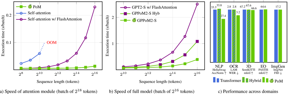Figure 1. Polynomial Mixer ( PoM). Inference time on an H100 as a function of sequence length, shown for the PoM module alone (a) and within a full Transformer pipeline (b). PoM scales nearly linearly and is significantly faster than self-attention for long sequences, even with FlashAttention. As measured for NLP, OCR, 3D point cloud segmentation, Earth Observation analysis, and image generation (c), replacing attention with PoM or hybrid variants preserves accuracy while improving scalability. <details> <summary>Image 1 Details</summary>  ### Visual Description ## Line Charts and Bar Graph: Execution Time and Performance Comparison ### Overview The image contains three visualizations comparing computational efficiency and performance across different attention mechanisms and model architectures. Part (a) analyzes attention module speed, part (b) evaluates full model speed, and part (c) compares domain-specific performance metrics. --- ### Components/Axes #### Part (a): Speed of Attention Module - **X-axis**: Sequence length (tokens) from 2⁸ to 2¹⁶ (logarithmic scale) - **Y-axis**: Execution time (s/batch) - **Legend**: - Green squares: PoM - Blue circles: Self-attention - Purple circles: Self-attention w/ FlashAttention - **Annotations**: "OOM" (Out of Memory) marker at 2¹⁶ for Self-attention #### Part (b): Speed of Full Model - **X-axis**: Sequence length (tokens) from 2¹⁰ to 2¹⁶ (logarithmic scale) - **Y-axis**: Execution time (s/batch) - **Legend**: - Purple circles: GPT2-S w/ FlashAttention - Green squares: GPPoM2-S Hyb - Green diamonds: GPPoM2-S #### Part (c): Performance Across Domains - **X-axis**: Domains (NLP, OCR, 3D, EO, ImgGen) - **Y-axis**: Performance metrics (percentage values) - **Legend**: - Blue bars: Transformer - Green bars: Hybrid - Green bars with checkmark: PoM --- ### Detailed Analysis #### Part (a): Speed of Attention Module - **Trend**: - PoM (green) remains nearly flat across all sequence lengths. - Self-attention (blue) increases gradually, with a sharp rise at 2¹⁶. - Self-attention w/ FlashAttention (purple) follows Self-attention until 2¹⁶, then spikes dramatically. - **Key Data Points**: - At 2⁸: PoM ≈ 0.005, Self-attention ≈ 0.01, FlashAttention ≈ 0.01 - At 2¹⁶: PoM ≈ 0.02, Self-attention ≈ 0.15, FlashAttention ≈ 0.25 (OOM noted) #### Part (b): Speed of Full Model - **Trend**: - GPPoM2-S (green diamonds) remains stable across sequence lengths. - GPPoM2-S Hyb (green squares) increases slightly. - GPT2-S w/ FlashAttention (purple) follows Hyb until 2¹⁶, then spikes. - **Key Data Points**: - At 2¹⁰: GPPoM2-S ≈ 0.05, GPPoM2-S Hyb ≈ 0.06, GPT2-S ≈ 0.07 - At 2¹⁶: GPPoM2-S ≈ 0.1, GPPoM2-S Hyb ≈ 0.15, GPT2-S ≈ 0.3 (OOM implied) #### Part (c): Performance Across Domains - **Trend**: - PoM (green checkmark) outperforms Transformer and Hybrid in most domains. - Hybrid (green) and Transformer (blue) show mixed performance. - **Key Data Points**: - **NLP**: Transformer 33.3%, Hybrid 27.4%, PoM 33.8% - **OCR**: Transformer 2.8%, Hybrid 2.8%, PoM 3.2% - **3D**: Transformer 67.2%, Hybrid 67.6%, PoM 64.6% - **EO**: Transformer 64.6%, Hybrid 66.6%, PoM 64.6% - **ImgGen**: Transformer 17.2%, Hybrid 17.2%, PoM 17.2% --- ### Key Observations 1. **Memory Constraints**: Self-attention and FlashAttention exhibit OOM at 2¹⁶ tokens, while PoM remains stable. 2. **Efficiency**: PoM maintains consistent execution times across sequence lengths, unlike Self-attention variants. 3. **Domain Performance**: PoM matches or exceeds Transformer/Hybrid in most domains, with notable exceptions in 3D and EO. --- ### Interpretation - **Attention Mechanisms**: PoM's stability suggests superior scalability for long sequences, while FlashAttention's OOM limitation highlights memory bottlenecks. - **Model Speed**: GPPoM2-S variants outperform GPT2-S with FlashAttention for shorter sequences but face similar OOM risks at 2¹⁶. - **Domain Adaptability**: PoM's consistent performance across domains implies robustness, whereas Transformer/Hybrid show domain-specific trade-offs (e.g., 3D/EO performance dips for PoM). - **Practical Implications**: For applications requiring long-sequence processing (e.g., genomics, long-form text), PoM may be preferable despite slightly higher baseline costs. Hybrid/Transformer combinations offer domain-specific optimizations but require careful memory management. </details> ## Abstract This paper introduces the Polynomial Mixer (PoM), a novel token mixing mechanism with linear complexity that serves as a drop-in replacement for self-attention. PoM aggregates input tokens into a compact representation through a learned polynomial function, from which each token retrieves contextual information. We prove that PoM satisfies the contextual mapping property , ensuring that transformers equipped with PoM remain universal sequenceto-sequence approximators. We replace standard selfattention with PoM across five diverse domains: text generation, handwritten text recognition, image generation, 3D modeling, and Earth observation. PoM matches the performance of attention-based models while drastically reducing computational cost when working with long sequences. The code is available at https://github. com/davidpicard/pom . ## 1. Introduction One apple is a supper; one apple is life. -Les Misérables, Book Fourth , Victor Hugo Multi-Head Attention (MHA) [70] is the key ingredient to recent advances in AI, powering large language models [21, 58, 67], generative models for images and videos [52, 54, 76], as well as breakthroughs in computer vision [20] and speech processing [2, 11, 19, 80]. However, MHA has a quadratic complexity with respect to the input sequence length, severely limiting the attainable context size. Numerous sub-quadratic approximations have been proposed, yet most trade efficiency for either performance or generality. For instance, Linformer [72] requires a fixed sequence length, while State Space Models (SSMs) [55] impose a causal ordering that does not apply to all modalities. In this paper, we question whether quadratic complexity is truly necessary to match the performance of MHA on sequence-to-sequence tasks. Our approach draws inspiration from the long-standing use of high-order moments and polynomial features in representation learning [37, 57], which we revisit here as an alternative to attention. We introduce the Polynomial Mixer (PoM), a novel module with linear complexity that achieves comparable performance to MHA across diverse, real-world tasks. PoM aggregates the entire input sequence into a compact representation using a learned polynomial function, computed in linear time. Each token then retrieves relevant contextual information from this summary through a cross-attention-like mechanism. The contextual mapping property [77] is a key aspect of MHA enabling modern transformers to be universal sequence-to-sequence approximators. This property is rarely satisfied by standard neural network components; for instance, MLPs, CNNs, and SSMs do not exhibit it. We show that our proposed Polynomial Mixer (PoM) has the contextual mapping property, allowing it to replace attention blocks in transformers without sacrificing expressivity. We validate the efficiency and expressivity of PoM across five diverse tasks from different domains: text generation, image generation, optical character recognition, 3D point cloud segmentation, and multi-temporal satellite images analysis. As shown in Fig. 1, PoM matches the performance of MHA while providing a significant speedup on long sequences. Our main contributions are: - We propose PoM, a token mixing mechanism with linear complexity in the number of tokens. - Weprove that PoM satisfies the contextual mapping property, ensuring transformers equipped with PoM remain universal sequence-to-sequence approximators. - We demonstrate that PoM achieves performance on par with MHA across five distinct domains, while being substantially more efficient. ## 2. Related Work Wereview prior work on efficient attention mechanisms and alternative architectures that aim to replace or bypass selfattention. Faster Attention. Since the introduction of Transformers [70], many efforts have been made to reduce the quadratic complexity of MHA [10, 43, 72]. Notably, methods like Reformer [43] use fast approximate neighbors to reduce the size of the attention matrix based on the assumption that most tokens will have zero attention. To go further, Linformer [72] proposes to compute an explicit low rank projection of the keys and the values to reduce the complexity of MHA from the size of the sequence n to an arbitrary chosen number k ≪ n . The main drawback of such approach is that n and k are fixed, which means that the model can no longer process sequences of varying length. With the advent of Large Language Models and their ability to process extremely long sequences [1, 21, 66], recent efforts have been put on more efficient implementations such as Flash-Attention [15, 17] or KV-cache [6, 51] which seem sufficient for text. However for visual content, the sequence length grows quadratically with the resolution. Because MHA is also quadratic in the number of tokens, this leads to quartic computational and memory complexity. Alternatives to Attention. Alternatively, some attempts have been made to remove the Multi-Head Attention entirely, such as in MLP-Mixer [68] and ResMLP [69] that replace MHA with simple projection on the transpose tensor ( i.e. , considering the sequence dimension as features). These approaches have been shown to obtain competitive results, but similarly to Linformer, they imply a fix sequence length since this length is now an intrinsic dimension of the projection in the transpose direction. More recently, StateSpace Models (SSM) [27, 28] have become the focus of recent work especially in language modeling [16, 25, 46, 84]. SSM are recurrent models, which is highly beneficial for language modeling because of the causal property of text: the complexity to generate the next token becomes constant. In visual content however, there is no such natural causality pattern in the spatial dimensions. Attempt to use such models for vision tasks have been successful [49, 55, 83], albeit at the cost of enforcing an arbitrary 1dimensional scan order of the tokens that does not encode well the 2D nature of an image. In image generation with diffusion [35, 75], since the model has to be iterated, this results in a doubly sequential processing (space and iterations) that does not benefit from the parallel nature of processing images. For video however, the causal aspect is natural over the time dimension, recurrent approaches may be more efficient. Overall, we question whether a linear time algorithm can achieve the performances of the quadratic attention without imposing causal constraints as SSMs or a fixed sequenced size as Linformer or ResMLP. ## 3. Method In this section, we first describe PoM, our proposed sequence-to-sequence drop-in replacement for MHA (Sec. 3.1). We then propose an extension to causal sequences (Sec. 3.2) and a theoretical analysis (Sec. 3.3) ## 3.1. 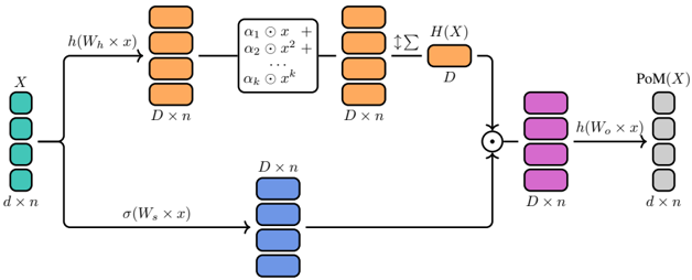Polynomial Mixer and Polymorpher Polynomial Mixer. We consider an input sequence of n tokens of dimension d , stored in a tensor X ∈ R d × n . Unlike MHA, which computes all pairwise interactions between tokens, the Polynomial Mixer relies on a shared state representation H ( X ) that serves as a common memory accessible to all tokens. This state aggregates information from the entire sequence after mapping tokens into a higherdimensional space R D through a learned polynomial function-hence the name Polynomial Mixer . Figure 2. Polynomial Mixer. An input sequence X of n tokens with dimension d follows two parallel paths. In the top path, each token is first expanded from dimension d to D , then transformed through a polynomial of degree k with coefficients α (all multiplications and exponentiations are element-wise). Dimension k is collapsed by summation, yielding a shared state H ( X ) ∈ R D . In the bottom path, each token produces gating coefficients in [0 , 1] D , which query information from H ( X ) via element-wise multiplication (broadcasted across n ). The result is finally projected back to the original dimension d . <details> <summary>Image 2 Details</summary>  ### Visual Description ## Neural Network Architecture Diagram: Multi-Layer Processing Flow ### Overview The diagram illustrates a multi-stage neural network architecture with input processing, hidden layers, summation operations, pooling, and output generation. The flow progresses from left to right, with color-coded components representing different processing stages. ### Components/Axes 1. **Input Layer (Teal)** - Dimensions: `d x n` - Represents raw input data `X` 2. **Hidden Layers (Orange)** - Dimensions: `D x n` - Labeled `h(W_h × x)` indicating activation function `h` applied to weights `W_h` and input `x` 3. **Summation Block (Black Box)** - Mathematical operation: `α₁·x + α₂·x² + ... + αₖ·xᵏ` - Combines weighted input terms with coefficients α₁ to αₖ 4. **Second Hidden Layer (Orange)** - Dimensions: `D x n` - Labeled `H(X)` indicating processed output from summation block 5. **Pooling Layer (Purple)** - Operation: `PoM(X)` (likely "Pooling of Maxima") - Reduces dimensionality while preserving key features 6. **Output Layer (Gray)** - Dimensions: `d x n` - Final processed output 7. **Activation Functions** - Sigmoid (`σ`) in blue layer - Rectified Linear Unit (`h`) in orange/purple layers ### Detailed Analysis - **Input Processing**: Raw data `X` (d x n) passes through initial hidden layer with activation `h(W_h × x)` - **Feature Combination**: Summation block applies polynomial-like combination of input features with learned coefficients - **Dimensionality Preservation**: Second hidden layer maintains `D x n` dimensions before pooling - **Spatial Reduction**: Pooling layer (`PoM(X)`) reduces spatial dimensions while retaining critical features - **Output Matching**: Final output matches input dimensions (`d x n`), suggesting regression/classification task ### Key Observations 1. **Architectural Symmetry**: Input and output dimensions match (`d x n`), while hidden layers use larger `D x n` dimensions 2. **Non-Linear Transformation**: Multiple activation functions (`h`, `σ`) introduce non-linearity 3. **Custom Operation**: Summation block implements explicit feature combination not typical in standard neural networks 4. **Dimensionality Control**: Pooling layer strategically reduces feature map size while preserving spatial hierarchy ### Interpretation This architecture appears designed for tasks requiring: - Feature extraction through multiple hidden layers - Explicit feature combination via the summation block (potentially for attention mechanisms or custom operations) - Spatial hierarchy preservation through controlled pooling - Output matching input dimensions for direct regression/classification The presence of both sigmoid and ReLU activations suggests a hybrid approach to non-linearity handling. The summation block's polynomial-like combination of features indicates intentional modeling of specific feature interactions, possibly for specialized tasks like time-series analysis or spatial pattern recognition. The pooling operation's "Maxima" focus suggests interest in dominant features rather than average values, common in computer vision applications. </details> Formally, the sequence X ∈ R d × n is summarized into a single representation H ( X ) ∈ R D × 1 , defined as a polynomial of degree k : ## 3.2. Polymorpher for Causal Sequences $$H ( X ) = \left[ \sum _ { p = 1 } ^ { k } a _ { p } o h ( x ) \right] _ { w _ { h } }$$ where D is the internal feature dimension, α ∈ R D × k are the polynomial coefficients, h is an activation function, ⊙ denotes the element-wise (Hadamard) product with broadcasting, and 1 is a vector of ones used to sum over the sequence dimension n . The exponentiation is also applied element-wise. The matrix W h ∈ R D × d is a learnable parameter that mixes dimensions to ensure H ( X ) is composed of inter-dimension polynomials instead of just monomials. Each token then queries the shared representation H ( X ) using the gating coefficient S ( X ) = σ ( W s X ) ∈ [0 , 1] D × n and the resulting information is projected back into the original space by W o : $$P _ { o } ( X ) = W _ { o } [ ( W _ { g } ^ { \circ } ) ]$$ where σ is the sigmoid function, and W o ∈ R d × D and W s ∈ R D × d are learnable parameters. All operations are linear in the sequence length n . PolyMorpher. Drawing inspiration from Transformer architectures, we define a PolyMorpher block P that alternates residual Polynomial Mixer and feed-forward layers: $$F ( X + P o M ( X ) , ( 3 )$$ where FF ( X ) denotes a standard two-layer feed-forward network. The PolyMorpher thus acts as a drop-in replacement for Transformer blocks based on MHA, fulfilling the same sequence-to-sequence mapping role. The key difference lies in its parametrization: while Transformers are configured by the number of heads and their dimension, the Polymorpher is defined by the degree k and the internal dimension D of its polynomial. We consider a sequence with a causal structure encoded by a binary mask M ∈ { 0 , 1 } n × n , where M s,t = 1 if and only if token s is allowed to use information from token t to update its representation. The Polynomial Mixer can be readily adapted to handle such causal dependencies by defining a distinct state representation H ( X ) for each time step of the sequence: $$H ( X ) = \sum _ { p = 1 } ^ { k } \alpha _ { p } \circ h ($$ Here, H ( X ) ∈ R D × n , and the formulation in Equation (2) remains unchanged. Causal Sequence. In the special case of causal sequences, the mask M is a lower triangular matrix. This allows computing the state representation at time step t , denoted H ( X ) t , through the following iterative process: $$\sum _ { s \leq t } | \sum _ { p = 1 } ^ { k } a _ { p } o _ { h } ( X ) ^ { p } | ,$$ $$= H ( X ) _ { t - 1 } + \left[ \sum _ { p = 1 } ^ { k } a _ { p } \circ h ( W _ { h } X ) ^ { p } \right] . ( 6 )$$ This formulation enables O (1) inference complexity in the autoregressive setting, a property shared with recurrent networks but not with transformers. Similar to SSMs, Polymorphers combine the advantages of both worlds: they can be trained on the entire sequence in parallel while supporting efficient recursive inference. Block Causal Sequence. Polymorphers can also model block-causal sequences, as found in spatio-temporal data such as videos or satellite image time series. In this setting, each token can attend to all tokens within the same frame, as well as to tokens from preceding frames. Let M denote a block-causal mask for a block size K : $$M _ { i , j } = 1 if j \leq | i / K ^ { }$$ The state representation H can then be computed as $$\sum _ { s = 1 } ^ { t / K } \sum _ { p = 1 } ^ { k } [ \sum _ { i = 1 } ^ { t / K } h ( W _ { h } , X ) ^ { p } ] .$$ This formulation allows processing tokens in blocks during inference, reducing memory requirements while preserving causal dependencies. ## 3.3. Theoretical Analysis We first show that PoM is equivariant , which means that permutations in the input sequence result in permuted outputs. This is a key property that made transformers popular and does not hold for other architectures like convolutions or recurrent networks. Proposition 3.1 (Permutation equivariance) . A Polynomial Mixer is permutation equivariant, i.e ., let X ∈ R d × n be a set of vectors and P a column permutation matrix, then PoM ( XP ) = PoM ( X ) P . Proof. For a permutation P , we have $$P _ { O } ( X P ) = W _ { 0 } [ σ ( W _ { s } ^ { - } ) ] . ( 9 )$$ We have that H ( XP ) = H ( X ) because the sum is permutation invariant, and σ ( W s XP ) = σ ( W s X ) P because σ is an element-wise operation. Noticing that H ( X ) 1 ⊤ has all identical columns allows us to move P outside of the brackets to conclude the proof. More importantly, we can also prove a universal approximation theorem for Polymorphers similar to what is well known for Transformers [77]. As the polynomial mixer is equivariant, it requires the use of positional encoding (learned for simplicity reasons), which also underlines the similarity between PoM and MHA. We use the following standard definition of distance between functions that map sequences to sequences. Given two functions f and g : R d n → R d n and an integer A ≤ p ≤ ∞ , we define the distance d p as: The following theorem holds: Theorem 3.2 (Universal approximation) . Let 1 ≤ p ≤ ∞ and ϵ > 0 , then for any given f ∈ F the set of continuous functions that map a compact domain in R d × n to R d × n , there exists a Polymorpher g with learned positional encoding such that d p ( f, g ) ≤ ϵ . The proof follows exactly the same scheme as in [77], where most of the heavy lifting is done by the feed-forward networks. Their main argument is to show that MHA can map every token in the sequence to a unique value that depends on the entire sequence, and then the feed-forward blocks can map those unique values to the desired output. In our case, we just have to ensure that the Polynomial Mixer has the same properties as MHA, which is obtained using the following lemma: Lemma 3.3 (Contextual mapping (informal)) . There exists k > 0 for which any Polynomial Mixer q of degree k is a contextual mappings on R d × n , that is: - For any X ∈ R d × n with different entries, q ( X ) has different entries. - For any X,X ′ ∈ R d × n that differ at least by one element, then all entries of q ( L ) and q ( L ′ ) are different. The proof is deferred to the appendix and primarily uses the fact that a sufficiently high degree polynomial is uniquely defined by a sequence of point-wise evaluation. As noted in [77], having the contextual mapping property is not so common as it requires to summarize uniquely the context while preserving the identity of the current token. With these results, we show that a Polymorpher is as potent as a Transformer for sequence modeling. ## 3.4. Complexity and Efficiency Analysis When is PoM faster than MHA? For a sequence of length n , the cost of PoM breaks down as follows: 2 dDn multiplications for input projections, nkD multiplications to compute the polynomial, and and nD sums to aggregate it. The selection operation costs nD multiplications, and the output projection costs nDd . Assuming that the cost of additions is negligible in front of that of multiplications, this gives us a total cost of 3 ndD +( k +1) nD multiplications. In comparison, the cost of input projections for attention is 3 nd 2 multiplications. Then, the cost of computing the attention matrix is dn 2 multiplications and aggregating the values is also dn 2 multiplications. Finally, the output projection cost is nd 2 . This sums to a total cost of 4 nd 2 +2 dn 2 . Solving for n leads to PoM being faster when $$n \geq \frac { D ( 3 d + k + 1 ) - 4 d ^ { 2 } } { 2 d } ,$$ with the polynomial degree k and the hidden dimension D setting different trade-offs. In our experiments, we found that D = 2 d and k = 2 is sufficient to match the performances of attention. In this case, PoM has a complexity advantage for n ≥ d +3 which usually amounts to sequences of sizes greater than 1k tokens ( d = 512 -1024 ). 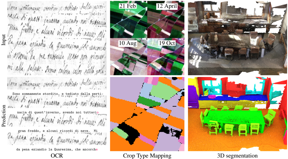Below this range, highly optimized attention kernels can remain competitive; however, as n grows, the cost of MHA increases quadratically while PoM grows linearly, making Figure 3. Evaluation Across Domains. We evaluate PoM on various tasks from multiple domains, simply replacing some or all the self-attention blocks in SOTA Transformer-based models. Left : For OCR, given a page of handwritten text (top) split into lines, the goal is to recognize each character and group them into words (bottom). Middle : For Earth observation, given a time series of satellite images (top), the goal is to classify each pixel as a crop type by the end of the series (bottom). Right : For 3D segmentation, given a 3D point cloud (top), the goal is to classify each point according to classes (bottom). <details> <summary>Image 3 Details</summary>  ### Visual Description ## Screenshot: OCR and 3D Segmentation Workflow ### Overview The image demonstrates a three-stage process: 1. **Input**: Handwritten Italian text 2. **Prediction**: OCR output with corrections 3. **Output**: - Temporal progression of a room's appearance (21 Feb, 12 April, 10 Aug, 19 Oct) - Color-coded 3D segmentation of a room interior ### Components/Axes - **Columns**: - **Input**: Handwritten text in Italian (top-left) - **Prediction**: OCR results with corrections (bottom-left) - **Output**: - **Temporal Images**: Four dated snapshots (21 Feb, 12 April, 10 Aug, 19 Oct) - **3D Segmentation**: Color-coded room interior (right column) - **Legend**: Located on the right of the 3D segmentation, mapping colors to objects: - Green: Chairs - Red: Walls - Blue: Windows - Yellow: Table - Orange: Floor ### Detailed Analysis #### Input Column - **Text**: Handwritten Italian script (unreadable due to resolution, but contains phrases like "Sono sommamente stordito" and "da pena ezziando la Quaresima"). - **OCR Prediction**: Machine-transcribed text with corrections (e.g., "gran freddo" vs. "gran freddo"). Corrections are highlighted in red. #### Output Column - **Temporal Images**: - **21 Feb**: Green and purple plaid pattern. - **12 April**: Green and red plaid pattern. - **10 Aug**: Green and black plaid pattern. - **19 Oct**: Green and purple plaid pattern. - **3D Segmentation**: - **Color Coding**: - Green: Chairs (12 chairs visible) - Red: Walls (4 walls) - Blue: Windows (2 windows) - Yellow: Table (1 table) - Orange: Floor (1 floor) ### Key Observations 1. **OCR Accuracy**: - Corrections in the Prediction column suggest the OCR model struggles with cursive handwriting and specific Italian words (e.g., "Quaresima" vs. "Quaresima"). 2. **Temporal Progression**: - The room's appearance changes minimally across dates, with consistent furniture placement but varying wall/floor colors. 3. **3D Segmentation**: - Color-coded segmentation demonstrates object recognition but lacks depth information (e.g., chairs are flat, not 3D). ### Interpretation - **OCR Limitations**: The model's errors highlight challenges in processing stylized handwriting and domain-specific vocabulary (e.g., "Quaresima" = Easter period). - **3D Segmentation**: The color-coded output suggests a focus on semantic segmentation rather than geometric accuracy. The absence of depth data implies a 2.5D representation. - **Temporal Context**: The dated images may represent different stages of a renovation or seasonal changes, though the minimal visual differences suggest limited temporal variation. ## Italian Text Transcription **Input Column**: - "Sono sommamente stordito, e tediatto dalla parti- nalla di quest'inverno, avendo noi tuttavio gran freddo, e alcuni ricordi di neve. Mi da pena ezziando la Quaresima, che ancorhe..." **Prediction Column**: - Corrections: - "gran freddo" (original: "gran freddo") - "Quaresima" (original: "Quaresima") ## Chart/Diagram Type - **Primary**: Screenshot of a technical workflow visualization. - **Secondary**: Color-coded 3D segmentation diagram. </details> PoM significantly more efficient for long-context applications. This trend is especially pronounced in settings such as high-resolution image or video modeling, geospatial sequences, or autoregressive generation over long documents, where PoM's linear scaling yields substantial speedups. Comparing with Flash-Attention. Highly optimized attention implementations such as FlashAttention [18] achieve near-linear runtime for moderate sequence lengths through clever memory management and custom CUDA kernels. In contrast, our PoM implementation is written entirely in high-level PyTorch, requiring no compilation or specialized code. Despite this, PoM already demonstrates superior scalability for long sequences and large images, but remain slower for smaller ones. We argue that directly comparing new methods with highly-optimized implementations should be interpreted cautiously. This paper presents a proof of concept, showcasing PoM's efficiency and versatility across several domains and multiple tasks. We expect further gains with dedicated low-level optimization which are out of the scope of our proof of concept. ## 4. Experiments We evaluate PoM across a diverse set of tasks and modalities: natural language processing (Sec. 4.1), optical character recognition (Sec. 4.2), Earth observation analysis (Sec. 4.3), 3D point cloud segmentation (Sec. 4.4), and image generation (Sec. 4.5). Examples for the visual tasks are shown in Figure 3. This diversity highlights that PoM can serve as a drop-in, compute-efficient replacement for the standard self-attention transformer block. We also explore the validity of hybrid models which retain some attention layers. In all our experiments, we do not introduce major architectural changes compared to the original models, but we parametrize PoM and the MLP in the blocks so as to keep the total number of parameters close to the original one. We also do not deviate from their original training recipe, except for experiments where changing the number of tokens would create training instabilities both for attention and PoM. ## 4.1. Natural Language Processing Setting. We train 125M GPT-2 models on 15B tokens from FineWeb [56], following the nanoGPT setup [40]. We evaluate models using validation loss, accuracy on the fol- (a) Performance. Comparison of GPT2 trained on 15B tokens from FineWeb and its GPPoM2 version. | Model | Val Loss | ↓ ARC-E Acc.Norm | HellaSwag Acc.Norm ↑ | Winogrande ↑ MMLU ↑ | Winogrande ↑ MMLU ↑ | |-----------------|------------|--------------------|------------------------|-----------------------|-----------------------| | Model | Val Loss | ↓ ARC-E Acc.Norm | HellaSwag Acc.Norm ↑ | Acc. | Acc. | | GPT2-S (OpenAI) | - | 42.8 | 31.6 | 50.0 | 26.1 | | GPT2-S 12MHA | 3.29 | 29.4 | 33.3 | 49.4 | 24.6 | | GPPoM2-S | 3.88 | 28.7 | 27.4 | 48.6 | 25.5 | | GPPoM2-S Hyb. | 3.31 | 29.0 | 33.8 | 51.9 | 25.6 | (b) Efficiency. Token processing speed (in k-tokens/s) at which models are processing (forward) sequences of varying length. | Sequence length | 1k | 4k | 16k | 32k | |-------------------|-------|-------|--------|--------| | GPT2-SMHA | 572.3 | 294.6 | 99.3 | 52.4 | | GPPoM2-S k = 2 | 995.7 | 893.1 | 624.2 | 447.5 | | k = 3 | 993.5 | 890.5 | 622.79 | 445.78 | | k = 5 | 995.6 | 890.2 | 617.1 | 439.51 | | GPPoM2-S Hyb. | 796.1 | 533.4 | 227.8 | 128.7 | | Mamba | 56.4 | 56.1 | 56.8 | 56.7 | Table 1. Natural Language Processing. lowing benchmarks: ARC-E [12], HellaSwag [78], Winogrande [61], and MMLU [32]. We measure generation speed measured as the time to produce the last token in sequences of varying lengths. Weconsider two configurations: (i) GPPoM2 , where every self-attention block is replaced by a Polymorpher, and (ii) GPPoM2 Hyb. , where pairs of self-attention blocks are replaced by one Polymorpher and one local-attention block with a causal context limited to the last 128 tokens. This hybrid design combines the global receptive field of PoM's state representation with the local, fine-grained modeling of attention; this is conceptually similar to how LSTMs blend long- and short-range dependencies [34]. Moreover, the hybrid architecture preserves a constant computational cost during autoregressive inference, since the local attention context is fixed. Results. As reported in Tab. 1a, GPPoM2 achieves performance comparable, though slightly below, that of fullattention Transformers. It is worth noting that all training hyperparameters were tuned specifically for standard Transformers and we did not change the training recipe. In contrast, the Hybrid GPPoM matches, and occasionally surpasses, the performance of GPT2-S, including the checkpoint released by OpenAI that was trained on an order of magnitude more data. Both GPPoM variants are substantially mode efficient than Transformers, owing to their linear-time complexity. We show in Table 1b the average speed for a forward pass on a fix token budget (from 128 batches of 1024 tokens to 4 batches of 32 k tokens), using custom triton kernels. PoM-based models are even substancially faster than Mamba, which only beats attention at very long sequence lengths due to the optimization in FlashAttention. The degree k does not have impact on the speed. Table 2. Optical Character Recognition. We compare HTRVT and HTR-VPoM on LAM single line and LAM multiline dataset. We report the Character Error Rate (CER), Word Error Rate (WER), and throughput (lines/s). The multiline experiments are trained for half the steps. | | #Params | Performance | Performance | Throughput | |---------------------|-----------|---------------|---------------|--------------| | Model | × 10 6 | CER ↓ | WER ↓ | lines/s | | LAM HTR-VT HTR-VPoM | 53.5 | 2.8 | 7.4 | 620.2 | | | 53.7 | 3.2 | 9.0 | 623.3 | | HTR-VPoM Hyb. | 53.5 | 2.8 | 7.5 | 622.7 | | LAM-Mul. HTR-VT | 54.9 | 3.3 | 9.3 | 598.4 | | HTR-VPoM | 55.2 | 3.7 | 10.9 | 675.5 | | HTR-VPoM Hyb. | 55.1 | 3.3 | 9.3 | 636.6 | ## 4.2. OCR Setting. We assess the effectiveness of PoM on a optical character recognition task (OCR). We use the SOTA HTRVT[45], a ViT based encoder only network, as our baseline. We conduct our experiments on the Ludovico Antonio Muratori (LAM) [7] dataset which consists of 25,823 lines in total. To showcase the benefits of PoM over standard attention we conduct two experiments, specifically, (i) Single line prediction and (ii) Multiple line prediction. Given the HTR-VT network only has four attention blocks we experiment with two type of PoM architecture: (i) HTR-VPoM: replacing all the attention layers from HTR-VT to PoM layers and (ii) HTR-VPoM Hybrid: alternating attention layers and PoM layers that perform full attention (no causal mask). Results. We report the scores in Tab. 2. For the singleline prediction experiments, PoM based architectures are on-par with attention regarding CER (character error rate) and WER (word error rate). However, given the sequence length is just 128 tokens, attention benefits from the low occupancy level of the GPU to compensate for its quadratic cost. To take advantage of the linear cost of PoM, we also consider predicting entire pages at a time, consisting of multiple lines. We concatenate lines from the same page to produce a wide image, similar to unrolling the page horizontally. This adds up to 16 lines, or about 2k tokens on average. On this multi-line setup, the performances of HTR-VT are slightly degraded (3.3 CER vs 2.8 originally) which may come from underfitting a larger input signal. HTR-VPoM Hybrid is on par with the original architecture, while increasing throughput by about 6%. HTR-VPoM obtains 0.4 worst CER but achieves a significant 12% speedup compared to Flash-Attention. Interestingly, the throughput of PoM models is higher in the multi-line setup than in the single line setup 1 , the opposite of attention models. This demonstrates the superior scalability of PoM compared to attention, even with Flash-Attention. 1 We assume this is due to the GPU being under-occupied and the latency having a bigger impact. Table 3. Satellite Image Time Series Segmentation. We compare of TSViT and TSViPoM on PASTIS fold 1. We report the overall accuracy (OA), mean IoU (mIoU), and throughput. | Model | #Params 6 | Performance | Performance | Throughput 2 | |-------------------|-------------|---------------|---------------|----------------| | | × 10 | OA ↑ | mIoU ↑ | km /s | | TSViT (paper) | 1.7 | 83.4 | 65.1 | - | | TSViT (retrained) | 1.7 | 82.8 | 64.6 | 7.2 | | TSViPoM | 1.7 | 82.7 | 64.6 | 26.3 | ## 4.3. Earth Observation Analysis Setting. We evaluate PoM on a standard geospatial task: crop type mapping from satellite multi-spectral image time series. Experiments are conducted on fold 1 of the PASTIS dataset [60], which contains Sentinel-2 time series with 10 spectral bands at a spatial resolution of 10 mper pixel. Each pixel is annotated with one of 19 crop type classes. We report overall accuracy (OA), mean Intersection over Union (mIoU), FLOPs, and throughput. Our baseline is the TSViT model [65], a state-of-theart architecture for supervised crop segmentation that alternates between temporal and spatial self-attention layers. We construct TSViPoM by replacing all Transformer blocks in TSViT with Polymorpher blocks, keeping the rest of the architecture unchanged. Results. TSViPoM achieves performance comparable to the TSViT baseline while offering a substantial speedupover 300% faster inference-demonstrating the efficiency of PoM as a drop-in replacement for attention in spatiotemporal modeling. This improvement is particularly relevant for geospatial applications, where inputs often span long temporal sequences, large spatial extents, and multiple spectral bands. In such settings, the quadratic scaling of self-attention becomes a major bottleneck, forcing practitioners to crop scenes, reduce temporal resolution, or downsample spectral information. By contrast, PoM's linear complexity allows the model to process long and high-dimensional sequences directly, preserving temporal continuity and spectral richness while maintaining fast and memory-efficient inference. ## 4.4. Point Cloud Segmentation Setting. We evaluate PoM for 3D point cloud semantic segmentation on two standard benchmarks: indoor scene understanding with ScanNet [14] and autonomous driving with SemanticKITTI [5]. Our baseline is the state-of-theart PointTransformerV3 (PTv3) [74], which serializes point clouds along space-filling curves that preserve local geometric continuity. These serialized sequences are hierarchically pooled to form a U-Net-like encoder-decoder architecture. At each scale, PTv3 applies several multi-head attention (MHA) layers with a local context of 1024 points, Table 4. 3D Point Cloud Segmentation. We compare PTv3 with PPoMv3 on two classic 3D datasets. | Model | #Param × 10 6 | Performance mIoU ↑ | Throughput 10 6 pts/s | |---------------------------------|-----------------|----------------------|-------------------------| | Scannet PTv3 PPoMv3 PPoMv3 Hyb. | 46.2 | 76.7 | 1.98 | | Scannet PTv3 PPoMv3 PPoMv3 Hyb. | 47.9 | 75.9 | 2.17 | | Scannet PTv3 PPoMv3 PPoMv3 Hyb. | 46.8 | 76.8 | 2.01 | | SKITTI PTv3 PPoMv3 PPoMv3 Hyb. | 46.2 | 67.2 | 1.12 | | SKITTI PTv3 PPoMv3 PPoMv3 Hyb. | 47.9 | 66.6 | 1.22 | | SKITTI PTv3 PPoMv3 PPoMv3 Hyb. 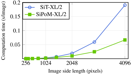| 46.8 | 67.5 | 1.15 | Figure 4. Computational Efficiency. We report the speed at generating image for various resolutions for SiT-XL/2 and its PoM counterpart SiPoM-XL/2. <details> <summary>Image 4 Details</summary>  ### Visual Description ## Line Graph: Computation Time vs. Image Size for SiT-XL/2 and SiPoM-XL/2 ### Overview The graph compares the computation time (in seconds per image) for two methods, **SiT-XL/2** (blue circles) and **SiPoM-XL/2** (green squares), across varying image sizes (256x256 to 4096x4096 pixels). Both methods show increasing computation time with larger images, but SiT-XL/2 exhibits a significantly steeper growth rate. --- ### Components/Axes - **X-axis**: Image side length (pixels) - Markers: 256, 1024, 2048, 4096 - **Y-axis**: Computation time (s/image) - Scale: 0.00 to 0.20 (increments of 0.05) - **Legend**: - **SiT-XL/2**: Blue circles (top-left corner) - **SiPoM-XL/2**: Green squares (top-left corner) --- ### Detailed Analysis 1. **SiT-XL/2 (Blue Circles)**: - **256px**: ~0.005s/image - **1024px**: ~0.01s/image - **2048px**: ~0.03s/image - **4096px**: ~0.19s/image - **Trend**: Exponential growth. The slope steepens dramatically between 2048px and 4096px. 2. **SiPoM-XL/2 (Green Squares)**: - **256px**: ~0.005s/image - **1024px**: ~0.005s/image - **2048px**: ~0.005s/image - **4096px**: ~0.06s/image - **Trend**: Linear growth. Computation time remains nearly constant until 4096px, where it rises modestly. --- ### Key Observations - **SiT-XL/2** computation time increases by **~38x** from 256px to 4096px. - **SiPoM-XL/2** computation time increases by **~12x** over the same range. - At 4096px, SiT-XL/2 is **~3.2x slower** than SiPoM-XL/2. - Both methods start with identical computation times at 256px. --- ### Interpretation The data highlights a critical efficiency disparity between the two methods. **SiPoM-XL/2** demonstrates superior scalability, maintaining near-constant computation time across image sizes, while **SiT-XL/2** becomes prohibitively slow for high-resolution images (e.g., 4096px). This suggests SiPoM-XL/2 may be preferable for applications requiring processing of large images, whereas SiT-XL/2 might be limited to smaller resolutions. The exponential growth of SiT-XL/2 raises questions about its algorithmic complexity (e.g., O(n²) vs. O(n log n) for SiPoM-XL/2). </details> a limit imposed by the quadratic cost of attention and GPU memory constraints. We investigate two PoM-based replacements for the attention modules: (i) PPoMv3 , which replaces all MHA layers with PoM while keeping the same context length, and (ii) PPoMv3-Hybrid , which alternates MHA layers, and PoM layers with a context window of 4096 points in the two highest-resolution stages of the U-Net. Results. Results are reported in Tab. 4. The hybrid PPoMv3 matches or slightly surpasses PTv3 on both datasets while reducing computation time by 2%. Pure PoM models are up to 10% faster than Flash-Attention, with only a minor drop in accuracy. A practical advantage of PoM's linear complexity is that entire point clouds can be processed in memory without chunking. While this does not translate into accuracy gains on standard CV benchmarks, it is a significant benefit for large-scale industrial applications where clean spatial partitioning such as single rooms is not applicable. ## 4.5. Class-Conditional Image Generation Setting. We evaluate PoM on a class-conditional image generation task. For that matter, we take the popular SiT architecture [52] and replace all Attention blocks with PoM blocks. We use the AdaLNZero strategy to condition the network on the class. 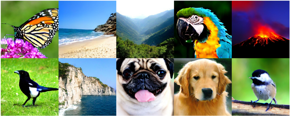We consider 2 sizes of models, Figure 5. Qualitative Results on Class-Conditional Generation resolution. We use classifier-free guidance with ω = 6 . <details> <summary>Image 5 Details</summary>  ### Visual Description ## Photo Grid: Diverse Natural and Animal Scenes ### Overview The image is a 3x3 grid of nine distinct photographs, each depicting a unique natural scene, animal, or landscape. No textual elements (labels, legends, axis titles) are present in the image. The grid is evenly spaced, with each photograph occupying its own square. ### Components/Axes - **Grid Structure**: - **Rows**: 3 rows (top, middle, bottom). - **Columns**: 3 columns (left, center, right). - **Photograph Descriptions**: 1. **Top-Left**: A monarch butterfly (orange, black, and white wings) perched on purple flowers. 2. **Top-Center**: A sandy beach with turquoise waves and a rocky cliff in the background. 3. **Top-Right**: A volcanic eruption at night, with glowing red lava and dark smoke against a starry sky. 4. **Middle-Left**: A black-and-white magpie standing on green grass. 5. **Middle-Center**: A steep, white limestone cliff overlooking a calm blue sea. 6. **Middle-Right**: A pug dog with a wrinkled face, black mask, and tongue out. 7. **Bottom-Left**: A golden retriever with golden fur and dark eyes. 8. **Bottom-Center**: A black-capped chickadee perched on a wooden branch. 9. **Bottom-Right**: A vibrant blue-and-yellow macaw with a green head and black beak. ### Detailed Analysis - **Top Row**: - **Butterfly**: Monarch butterfly (*Danaus plexippus*) with intricate wing patterns, resting on a cluster of small purple flowers. - **Beach**: Coastal scene with foamy waves lapping against pale sand; the cliff adds a rugged contrast. - **Volcano**: Active eruption with lava flows and ash clouds, suggesting a dynamic geological event. - **Middle Row**: - **Magpie**: Glossy black body with white wing patches, standing alert on grass. - **Cliff**: Vertical limestone formation with stratified layers, reflecting geological erosion. - **Pug**: Close-up of a pug’s face, emphasizing its wrinkled skin and expressive eyes. - **Bottom Row**: - **Golden Retriever**: Fluffy golden coat, soft fur texture, and friendly demeanor. - **Chickadee**: Small bird with black cap, white cheeks, and gray wings, gripping a branch. - **Macaw**: Tropical parrot with iridescent blue wings, yellow chest, and a curved black beak. ### Key Observations - **Diversity**: The grid showcases a mix of flora, fauna, and geological features, emphasizing biodiversity. - **Color Contrast**: Vibrant colors (e.g., macaw, volcano) stand out against neutral tones (e.g., cliffs, sand). - **Arrangement**: The grid balances natural and animal subjects, with no repetition of themes. ### Interpretation The grid likely serves as a visual collage to highlight the beauty and variety of nature and wildlife. The absence of text suggests the focus is on imagery rather than data or narrative. The juxtaposition of serene landscapes (beach, cliffs) with dynamic elements (volcano, butterfly) creates a thematic contrast between tranquility and activity. The inclusion of domesticated animals (pug, golden retriever) alongside wild species (macaw, chickadee) may imply a connection between human and natural worlds. **Note**: No numerical data, trends, or textual annotations are present in the image. The description is based solely on visible photographic content. </details> Table 5. Class-Conditional Image Generation . We compare SiT [52] with SiPoM trained on ImageNet for generating images of resolution 256 2 for a batch size of 1024. | Model | #Param × 10 6 | Performance FID ↓ | Throughput img/s | |------------|-----------------|---------------------|--------------------| | SiT-L/2 | 458 | 18.8 | 9842 | | SiPoM-L/2 | 414 | 17.6 | 11,954 | | SiT-XL/2 | 675 | 17.2 | 4041 | | SiPoM-XL/2 | 609 | 17.2 | 8146 | namely SiT-L and SiT-XL with a patch-size of 2, leading to our PoM variant named SiPoM-L/2 and SiPoM-XL/2 respectively. The training is performed on ImageNet at 256 resolution, with the same training parameters as in the original paper. The performances are evaluated with FID as is standard for this task. The efficiency is measured as throughput, which is the number of images per second that can be processed by a forward pass of the network for a batch size of 1024 images. Quantitative results We compare the results of our SiPoM models to the original scores from [52] on Table 5. Our SiPoM variants achieve the same visual fidelity as the original attention-based models, as measured by the FID. We also measure the throughput of the SiT-XL/2 and the SiPoM-XL/2 models at various resolution, which we report in Figure 4. As excepted, SiPoM becomes much more efficient than its attention-based counterpart at higher resolutions, starting at 1024 pixels per side. This is easily explain by the number of tokens growing quadratically with the resolution of the images, leading to longer sequences which further accentuate the gap between linear cost of PoM and . Images sampled from SiPom-XL/2 with different classes at 256 the quadratic cost of attention. Qualitative results We show images sampled from SiPoM-XL/2 in Figure 5. The images are sampled using Classifier Free Guidance with ω = 6 . The visual quality of the images is on par with equivalent models from the literature. This validates that SiPoM-XL/2 is able to produce the same quality of pictures as its attention counterpart. ## 5. Conclusion We introduced PoM , the Polynomial Mixer , a neural network building block that serves as a drop-in, efficient replacement for self-attention in Transformer architectures. PoM combines linear complexity with the universal sequence-to-sequence approximator . We validated PoM across five diverse domains-natural language processing, Earth observation, 3D point cloud segmentation, optical character recognition, and image generation. We demonstrate that hybrid PoM/self-attention architectures consistently match or surpass the performance of full-attention models while offering superior speed and scalability. These properties make PoM a compelling choice for long-sequence applications such as high-definition video generation or multimodal large language models, which could greatly benefit from its O (1) inference under causal masking. While large-scale experiments remain beyond our current computational scope, PoM lays the groundwork for the next generation of efficient, general-purpose, attentionfree sequence models. ## 6. Acknowledgment This work was supported by ANR project sharp ANR-23PEIA-0008 in the context of the PEPR IA. This project was provided with computing and storage resources by GENCI at IDRIS thanks to the grants 2025-A0191013085 and 2025-A0181016234 on the supercomputer Jean Zay's H100 partition. The authors would like to thank Vincent Lepetit, Gül Varol and Dimitris Samaras for their insightful comments and suggestions. ## References - [1] Josh Achiam, Steven Adler, Sandhini Agarwal, Lama Ahmad, Ilge Akkaya, Florencia Leoni Aleman, Diogo Almeida, Janko Altenschmidt, Sam Altman, Shyamal Anadkat, et al. GPT-4 technical report. arXiv:2303.08774 , 2023. - [2] Alexei Baevski, Yuhao Zhou, Abdelrahman Mohamed, and Michael Auli. wav2vec 2.0: A framework for self-supervised learning of speech representations. NeurIPS , 2020. - [3] Xingjian Bai and Luke Melas-Kyriazi. Fixed point diffusion models. In CVPR , 2024. - [4] Yogesh Balaji, Seungjun Nah, Xun Huang, Arash Vahdat, Jiaming Song, Qinsheng Zhang, Karsten Kreis, Miika Aittala, Timo Aila, Samuli Laine, Bryan Catanzaro, Tero Karras, and Ming-Yu Liu. eDiff-I: Text-to-image diffusion models with ensemble of expert denoisers. arXiv:2211.01324 , 2022. - [5] Jens Behley, Martin Garbade, Andres Milioto, Jan Quenzel, Sven Behnke, Cyrill Stachniss, and Jurgen Gall. SemanticKITTI: A dataset for semantic scene understanding of LiDAR sequences. In ICCV , 2019. - [6] William Brandon, Mayank Mishra, Aniruddha Nrusimha, Rameswar Panda, and Jonathan Ragan Kelly. Reducing transformer key-value cache size with cross-layer attention. NeurIPS , 2024. - [7] Silvia Cascianelli, Vittorio Pippi, Martin Maarand, Marcella Cornia, Lorenzo Baraldi, Christopher Kermorvant, and Rita Cucchiara. The LAM dataset: A novel benchmark for linelevel handwritten text recognition. In ICPR , 2022. - [8] Junsong Chen, Chongjian Ge, Enze Xie, Yue Wu, Lewei Yao, Xiaozhe Ren, Zhongdao Wang, Ping Luo, Huchuan Lu, and Zhenguo Li. Pixart-\ sigma: Weak-to-strong training of diffusion transformer for 4k text-to-image generation. In ECCV , 2024. - [9] Ting Chen and Lala Li. FIT: Far-reaching interleaved transformers. arXiv:2305.12689 , 2023. - [10] Rewon Child, Scott Gray, Alec Radford, and Ilya Sutskever. Generating long sequences with sparse transformers. arXiv:1904.10509 , 2019. - [11] Chung-Cheng Chiu, James Qin, Yu Zhang, Jiahui Yu, and Yonghui Wu. Self-supervised learning with randomprojection quantizer for speech recognition. In International Conference on Machine Learning . PMLR, 2022. - [12] Peter Clark, Isaac Cowhey, Oren Etzioni, Tushar Khot, Ashish Sabharwal, Carissa Schoenick, and Oyvind Tafjord. Think you have solved question answering? Ttry ARC, the AI2 reasoning challenge. arXiv:1803.05457 , 2018. - [13] Katherine Crowson, Stefan Andreas Baumann, Alex Birch, Tanishq Mathew Abraham, Daniel Z Kaplan, and Enrico Shippole. Scalable high-resolution pixel-space image synthesis with hourglass diffusion transformers. In Int. Conf. Mach. Learn. , 2024. - [14] Angela Dai, Angel X. Chang, Manolis Savva, Maciej Halber, Thomas Funkhouser, and Matthias Niessner. ScanNet: Richly-annotated 3D reconstructions of indoor scenes. In CVPR , 2017. - [15] Tri Dao. FlashAttention-2: Faster attention with better parallelism and work partitioning. ICLR , 2024. - [16] Tri Dao and Albert Gu. Transformers are SSMs: Generalized models and efficient algorithms through structured state space duality. In Int. Conf. Mach. Learn. , 2024. - [17] Tri Dao, Dan Fu, Stefano Ermon, Atri Rudra, and Christopher Ré. FlashAttention: Fast and memory-efficient exact attention with io-awareness. In NeurIPS , 2022. - [18] Tri Dao, Daniel Y. Fu, Stefano Ermon, Atri Rudra, and Christopher Ré. FlashAttention: Fast and memory-efficient exact attention with IO-awareness. In NeurIPS , 2022. - [19] Alexandre Défossez, Laurent Mazaré, Manu Orsini, Amélie Royer, Patrick Pérez, Hervé Jégou, Edouard Grave, and Neil Zeghidour. Moshi: A speech-text foundation model for realtime dialogue. arXiv:2410.00037 , 2024. - [20] Alexey Dosovitskiy, Lucas Beyer, Alexander Kolesnikov, Dirk Weissenborn, Xiaohua Zhai, Thomas Unterthiner, Mostafa Dehghani, Matthias Minderer, Georg Heigold, Sylvain Gelly, et al. An image is worth 16x16 words: Transformers for image recognition at scale. In ICLR , 2020. - [21] Abhimanyu Dubey, Abhinav Jauhri, Abhinav Pandey, Abhishek Kadian, Ahmad Al-Dahle, Aiesha Letman, Akhil Mathur, Alan Schelten, Amy Yang, Angela Fan, et al. The LLAMA 3 herd of models. arXiv:2407.21783 , 2024. - [22] Nicolas Dufour, Victor Besnier, Vicky Kalogeiton, and David Picard. Don't drop your samples! Coherence-aware training benefits conditional diffusion. In CVPR , 2024. - [23] Patrick Esser, Sumith Kulal, Andreas Blattmann, Rahim Entezari, Jonas Müller, Harry Saini, Yam Levi, Dominik Lorenz, Axel Sauer, Frederic Boesel, et al. Scaling rectified flow transformers for high-resolution image synthesis. In Int. Conf. Mach. Learn. , 2024. - [24] Peng Gao, Le Zhuo, Ziyi Lin, Chris Liu, Junsong Chen, Ruoyi Du, Enze Xie, Xu Luo, Longtian Qiu, Yuhang Zhang, et al. Lumina-T2X: Transforming text into any modality, resolution, and duration via flow-based large diffusion transformers. arXiv:2405.05945 , 2024. - [25] Paolo Glorioso, Quentin Anthony, Yury Tokpanov, James Whittington, Jonathan Pilault, Adam Ibrahim, and Beren Millidge. Zamba: A compact 7B SSM hybrid model. arXiv:2405.16712 , 2024. - [26] Aaron Gokaslan, A. Feder Cooper, Jasmine Collins, Landan Seguin, Austin Jacobson, Mihir Patel, Jonathan Frankle, Cory Stephenson, and Volodymyr Kuleshov. CommonCanvas: Open diffusion models trained on creative-commons images. In CVPR , 2024. - [27] Albert Gu, Karan Goel, and Christopher Re. Efficiently modeling long sequences with structured state spaces. In ICLR , 2021. - [28] Albert Gu, Isys Johnson, Karan Goel, Khaled Saab, Tri Dao, Atri Rudra, and Christopher Ré. Combining recurrent, convolutional, and continuous-time models with linear state space layers. In NeurIPS , 2021. - [29] Jiatao Gu, Shuangfei Zhai, Yizhe Zhang, Joshua M Susskind, and Navdeep Jaitly. Matryoshka diffusion models. In ICLR , 2023. - [30] Tiankai Hang and Shuyang Gu. Improved noise schedule for diffusion training. ICCV , 2024. - [31] Ali Hatamizadeh, Jiaming Song, Guilin Liu, Jan Kautz, and Arash Vahdat. DifFit: Diffusion vision transformers for image generation. In ECCV , 2024. - [32] Dan Hendrycks, Collin Burns, Steven Basart, Andy Zou, Mantas Mazeika, Dawn Song, and Jacob Steinhardt. Measuring massive multitask language understanding. In ICLR , 2021. - [33] Jonathan Ho, Ajay Jain, and Pieter Abbeel. Denoising diffusion probabilistic models. In NeurIPS , 2020. - [34] Sepp Hochreiter and Jürgen Schmidhuber. Long short-term memory. Neural computation , 1997. - [35] Vincent Tao Hu, Stefan Andreas Baumann, Ming Gui, Olga Grebenkova, Pingchuan Ma, Johannes Fischer, and Björn Ommer. ZigMa: A DiT-style zigzag Mamba diffusion model. In ECCV , 2024. - [36] Allan Jabri, David J Fleet, and Ting Chen. Scalable adaptive computation for iterative generation. In Int. Conf. Mach. Learn. , 2023. - [37] Pierre Jacob, David Picard, Aymeric Histace, and Edouard Klein. Metric learning with horde: High-order regularizer for deep embeddings. In ICCV , pages 6539-6548, 2019. - [38] Andrew Jaegle, Sebastian Borgeaud, Jean-Baptiste Alayrac, Carl Doersch, Catalin Ionescu, David Ding, Skanda Koppula, Daniel Zoran, Andrew Brock, Evan Shelhamer, et al. Perceiver IO: A general architecture for structured inputs & outputs. In ICLR , 2022. - [39] Jared Kaplan, Sam McCandlish, Tom Henighan, Tom B Brown, Benjamin Chess, Rewon Child, Scott Gray, Alec Radford, Jeffrey Wu, and Dario Amodei. Scaling laws for neural language models. arXiv preprint arXiv:2001.08361 , 2020. - [40] Andrej Karpathy. NanoGPT. https://github.com/ karpathy/nanoGPT , 2022. - [41] Tero Karras, Miika Aittala, Jaakko Lehtinen, Janne Hellsten, Timo Aila, and Samuli Laine. Analyzing and improving the training dynamics of diffusion models. In CVPR , 2024. - [42] Tero Karras, Miika Aittala, Jaakko Lehtinen, Janne Hellsten, Timo Aila, and Samuli Laine. Analyzing and improving the training dynamics of diffusion models. In CVPR , 2024. - [43] Nikita Kitaev, Lukasz Kaiser, and Anselm Levskaya. ReFormer: The efficient transformer. In ICLR , 2020. - [44] Seung Hyun Lee, Yinxiao Li, Junjie Ke, Innfarn Yoo, Han Zhang, Jiahui Yu, Qifei Wang, Fei Deng, Glenn Entis, Junfeng He, et al. Parrot: Pareto-optimal multi-reward reinforcement learning framework for text-to-image generation. In ECCV , 2025. - [45] Yuting Li, Dexiong Chen, Tinglong Tang, and Xi Shen. HTR-VT: Handwritten text recognition with vision transformer. Pattern Recognition , 2025. - [46] Opher Lieber, Barak Lenz, Hofit Bata, Gal Cohen, Jhonathan Osin, Itay Dalmedigos, Erez Safahi, Shaked Meirom, Yonatan Belinkov, Shai Shalev-Shwartz, et al. Jamba: A hybrid transformer-Mamba language model. ICLR , 2025. - [47] Yaron Lipman, Ricky TQ Chen, Heli Ben-Hamu, Maximilian Nickel, and Matthew Le. Flow matching for generative modeling. In ICLR , 2022. - [48] Xingchao Liu, Chengyue Gong, et al. Flow straight and fast: Learning to generate and transfer data with rectified flow. In ICLR , 2023. - [49] Yue Liu, Yunjie Tian, Yuzhong Zhao, Hongtian Yu, Lingxi Xie, Yaowei Wang, Qixiang Ye, and Yunfan Liu. Vmamba: Visual state space model, 2024. - [50] Yujian Liu, Yang Zhang, Tommi Jaakkola, and Shiyu Chang. Correcting diffusion generation through resampling. In CVPR , 2024. - [51] Shi Luohe, Zhang Hongyi, Yao Yao, Li Zuchao, and Zhao Hai. Keep the cost down: A review on methods to optimize LLM's KV-cache consumption. COLM , 2024. - [52] Nanye Ma, Mark Goldstein, Michael S Albergo, Nicholas M Boffi, Eric Vanden-Eijnden, and Saining Xie. SIT: Exploring flow and diffusion-based generative models with scalable interpolant transformers. In ECCV , 2024. - [53] Alexander Quinn Nichol and Prafulla Dhariwal. Improved denoising diffusion probabilistic models. In Int. Conf. Mach. Learn. , 2021. - [54] William Peebles and Saining Xie. Scalable diffusion models with transformers. In ICCV , 2023. - [55] Xiaohuan Pei, Tao Huang, and Chang Xu. EfficientVMamba: Atrous selective scan for light weight visual mamba, 2025. - [56] Guilherme Penedo, Hynek Kydlíˇ cek, Anton Lozhkov, Margaret Mitchell, Colin A Raffel, Leandro Von Werra, Thomas Wolf, et al. The fineweb datasets: Decanting the web for the finest text data at scale. NeurIPS , 2024. - [57] David Picard and Philippe-Henri Gosselin. Improving image similarity with vectors of locally aggregated tensors. In ICIP , pages 669-672, 2011. - [58] Alec Radford, Jeffrey Wu, Rewon Child, David Luan, Dario Amodei, Ilya Sutskever, et al. Language models are unsupervised multitask learners. OpenAI blog , 2019. - [59] Robin Rombach, Andreas Blattmann, Dominik Lorenz, Patrick Esser, and Björn Ommer. High-resolution image synthesis with latent diffusion models. In CVPR , 2022. - [60] Vivien Sainte Fare Garnot and Loic Landrieu. Panoptic segmentation of satellite image time series with convolutional temporal attention networks. ICCV , 2021. - [61] Keisuke Sakaguchi, Ronan Le Bras, Chandra Bhagavatula, and Yejin Choi. Winogrande: An adversarial winograd schema challenge at scale. Communications of the ACM , 2021. - [62] Yuyang Shi, Valentin De Bortoli, Andrew Campbell, and Arnaud Doucet. Diffusion Schrödinger bridge matching. In NeurIPS , 2024. - [63] Chenyang Si, Ziqi Huang, Yuming Jiang, and Ziwei Liu. FreeU: Free lunch in diffusion U-net. In CVPR , 2024. - [64] Yang Song, Jascha Sohl-Dickstein, Diederik P Kingma, Abhishek Kumar, Stefano Ermon, and Ben Poole. Score-based generative modeling through stochastic differential equations. In ICLR , 2021. - [65] Michail Tarasiou, Erik Chavez, and Stefanos Zafeiriou. ViTs for SITS: Vision transformers for satellite image time series. In CVPR , 2023. - [66] Gemini Team, Rohan Anil, Sebastian Borgeaud, JeanBaptiste Alayrac, Jiahui Yu, Radu Soricut, Johan Schalkwyk, Andrew M Dai, Anja Hauth, Katie Millican, et al. GEMINI: A family of highly capable multimodal models. arXiv:2312.11805 , 2023. - [67] Gemma Team, Morgane Riviere, Shreya Pathak, Pier Giuseppe Sessa, Cassidy Hardin, Surya Bhupatiraju, Léonard Hussenot, Thomas Mesnard, Bobak Shahriari, Alexandre Ramé, et al. Gemma 2: Improving open language models at a practical size. arXiv:2408.00118 , 2024. - [68] Ilya O Tolstikhin, Neil Houlsby, Alexander Kolesnikov, Lucas Beyer, Xiaohua Zhai, Thomas Unterthiner, Jessica Yung, Andreas Steiner, Daniel Keysers, Jakob Uszkoreit, et al. MLP-Mixer: An all-MLP architecture for vision. In NeurIPS , 2021. - [69] Hugo Touvron, Piotr Bojanowski, Mathilde Caron, Matthieu Cord, Alaaeldin El-Nouby, Edouard Grave, Gautier Izacard, Armand Joulin, Gabriel Synnaeve, Jakob Verbeek, et al. ResMLP: Feedforward networks for image classification with data-efficient training. IEEE TPAMI , 2022. - [70] Ashish Vaswani, Noam Shazeer, Niki Parmar, Jakob Uszkoreit, Llion Jones, Aidan N Gomez, Łukasz Kaiser, and Illia Polosukhin. Attention is all you need. In NeurIPS , 2017. - [71] Bram Wallace, Meihua Dang, Rafael Rafailov, Linqi Zhou, Aaron Lou, Senthil Purushwalkam, Stefano Ermon, Caiming Xiong, Shafiq Joty, and Nikhil Naik. Diffusion model alignment using direct preference optimization. In CVPR , 2024. - [72] Sinong Wang, Belinda Z Li, Madian Khabsa, Han Fang, and Hao Ma. LinFormer: Self-attention with linear complexity. arXiv:2006.04768 , 2020. - [73] Fanyue Wei, Wei Zeng, Zhenyang Li, Dawei Yin, Lixin Duan, and Wen Li. Powerful and flexible: Personalized text- to-image generation via reinforcement learning. In ECCV , 2024. - [74] Xiaoyang Wu, Li Jiang, Peng-Shuai Wang, Zhijian Liu, Xihui Liu, Yu Qiao, Wanli Ouyang, Tong He, and Hengshuang Zhao. Point Transformer v3: Simpler, faster, stronger. In CVPR , 2024. - [75] Jing Nathan Yan, Jiatao Gu, and Alexander M Rush. Diffusion models without attention. In CVPR , 2024. - [76] Zhuoyi Yang, Jiayan Teng, Wendi Zheng, Ming Ding, Shiyu Huang, Jiazheng Xu, Yuanming Yang, Wenyi Hong, Xiaohan Zhang, Guanyu Feng, et al. CogVideoX: Text-to-video diffusion models with an expert transformer. ICLR , 2025. - [77] Chulhee Yun, Srinadh Bhojanapalli, Ankit Singh Rawat, Sashank Reddi, and Sanjiv Kumar. Are transformers universal approximators of sequence-to-sequence functions? In ICLR , 2020. - [78] Rowan Zellers, Ari Holtzman, Yonatan Bisk, Ali Farhadi, and Yejin Choi. HellaSwag: Can a machine really finish your sentence? arXiv:1905.07830 , 2019. - [79] Xiaohua Zhai, Alexander Kolesnikov, Neil Houlsby, and Lucas Beyer. Scaling vision transformers. In CVPR , 2022. - [80] Yu Zhang, Wei Han, James Qin, Yongqiang Wang, Ankur Bapna, Zhehuai Chen, Nanxin Chen, Bo Li, Vera Axelrod, Gary Wang, et al. Google USM: Scaling automatic speech recognition beyond 100 languages. arXiv:2303.01037 , 2023. - [81] Yang Zhao, Yanwu Xu, Zhisheng Xiao, Haolin Jia, and Tingbo Hou. MobileDiffusion: Instant text-to-image generation on mobile devices. In ECCV , 2024. - [82] Zhenyu Zhou, Defang Chen, Can Wang, and Chun Chen. Fast ode-based sampling for diffusion models in around 5 steps. In CVPR , 2024. - [83] Lianghui Zhu, Bencheng Liao, Qian Zhang, Xinlong Wang, Wenyu Liu, and Xinggang Wang. Vision Mamba: Efficient visual representation learning with bidirectional state space model. arXiv:2401.09417 , 2024. - [84] Jingwei Zuo, Maksim Velikanov, Dhia Eddine Rhaiem, Ilyas Chahed, Younes Belkada, Guillaume Kunsch, and Hakim Hacid. Falcon Mamba: The first competitive attention-free 7B language model. arXiv:2410.05355 , 2024. ## PoM: A Linear-Time Replacement for Attention with the Polynomial Mixer ## Supplementary Material Table 6. Additional ablations and baselines. MHA throughput uses Flash-Attention, Performer uses torch\_geometric . | | ARC-easy Acc.Norm ↑ | HellaSwag Acc.Norm ↑ | Winogrande Acc. ↑ | Throughput 4096 tok., tok/s ↑ | |-----------------|-----------------------|------------------------|---------------------|---------------------------------| | PoM-hyb k=2 | 29 | 33.8 | 51.9 | 163 | | PoM-hyb k=3 | 29.5 | 33.4 | 49.6 | 161 | | PoM-hyb k=5 | 28.6 | 33.9 | 49.5 | 153 | | MHA | 29.4 | 33.3 | 49.4 | 42 | | Performer Mamba | 29.3 | training failed 30.8 | 48 | 59 384 | In this appendix, we report additional ablations (Sec. A) and analysis (Sec. B), and a proof of our main theoretical results (Sec. C). We also propose an extended related work in depth (Sec. D) and additional illustrations for the image generation experiment (Sec. E. ) ## A. Additional Ablations. Higher Orders k. We study the effect of increasing the polynomial degree k in Tab. 6. Higher-order polynomials provide a modest improvement, at the cost of a slight speed reduction. The limited impact is expected, as the sequences evaluated in classic benchmarks are relatively short and do not fully stress the model's representational capacity. As suggested by our theoretical analysis, higher-order interactions could become more critical for distinguishing longer sequences. Additional Baselines. We evaluate competing linear attention models and report their performance in Tab. 6. - Performer. We attempted to train a GPT2S model using Performer; however, both pytorch-performer and the Performer implementation from torch\_geometric systematically diverged, producing NaN losses after a few iterations. At present, we are not aware of a well-maintained Performer implementation suitable for large-scale language model training, which prevented a fair comparison. - Mamba. We trained a Mamba model of comparable size (124M parameters) on the NLP task; results are reported in Tab. 6. As expected, Mamba achieves excellent speed due to its O (1) complexity and dedicated CUDA kernel. PoM shares the same O (1) theoretical complexity, and we therefore expect that a dedicated CUDA implementation would yield comparable speedups. In terms of accuracy, however, Mamba performs below MHA and PoM on the evaluated benchmarks. We used the same classic training recipe inherited from attention-based models for all methods, which suggests that Mamba may require more tuning adaptation than PoM. We also observed that Mamba consumed approximately 4 × more memory during training, forcing smaller batch sizes and gradient accumulation, whereas PoM and MHA have a similar memory footprint. ## B. Additional Analysis. Comparison to FlashAttention. FlashAttention is a highly engineered implementation of attention, relying on custom CUDA kernels and carefully optimized memory management. In contrast, PoM is currently implemented entirely in high-level PyTorch, and yet already achieves consistent 2-4 × speedups across tasks, and in some settings (notably NLP, see Tab. 6, and image generation), PoM is faster than Flash-Attention. We therefore view these results as a conservative estimate of PoM's speed, and expect further gains with dedicated low-level optimization. Generalization Under Train-Test Length Mismatch. Since H ( x ) is obtained by pooling over tokens, its dimensionality is independent of the sequence length. In our NLP experiments, PoM is trained with a fixed sequence length of 2048 tokens (with padding), while evaluation on HellaSwag involves sequences ranging from 48 to 742 tokens, with no observable impact on performance. ## C. Proof of Lemma 3 We first need to show that set with different entries are mapped to different vectors. We first separate PoM into its two components: $$s ( X ) = σ ( W _ { s } X )$$ $$H ( X ) = \sum _ { p = 1 } ^ { k } a _ { p } \circ H ( X ) ^ { p }$$ $$X ) \circ H ( X ) = W _ { 0 } [ o ( W _ { s } )$$ Assuming ker( W o ) = ∅ , and noting that H k ( X ) is the same for every column, we just have to show that s ( X ) has different columns. This is easily achieved by having ker( W s ) = ∅ since σ is injective and the composition of injective functions is itself injective. Second, we have to show that sets that differ by at least one element are mapped to all different entries. To simplify notations, we will consider the special case where all matrices are the identity or an identity block positioned such as to perform submatrix selection. All the matrices can thus be removed from the formula. A similar argument can be made for matrices that are full rank as they preserve injectivity. We will also consider linear activations everywhere, which can be made as close as one wish by partitioning the image of the activation function and performing piecewise linear approximation. ̸ With this simplified version of PoM, we have to show that for 2 sets X,X ′ differing by at least one element (i.e., ∃ x ′ ∈ X ′ , ∀ x ∈ X,x = x ′ ), then there exist k such that ̸ $$\sum _ { i = 1 } ^ { n } x _ { i } ^ { k } + x \sum _ { i = 1 } ^ { n } x _ { i } . ( 1 5 )$$ Consider the functions P ( t ) and P ′ ( t ) defined as follows: $$P ( t ) = \sum _ { n = 1 } ^ { \infty } f _ { n }$$ $$P ^ { \prime } ( t ) = \sum _ { n = 0 } ^ { \infty } e ^ { - t }$$ ̸ Since X and X ′ differ by at least one element, there exists at least one x i ∈ X such that x i = x ′ i , ∀ x ′ i ∈ X ′ . This implies that the functions P ( t ) and P ′ ( t ) are not identical since are sums of exponentials with different bases. ̸ Since P ( t ) and P ′ ( t ) are different functions, there must exist some k for which P ( k ) = P ′ ( k ) . In other words, there exists a k such that: ̸ $$\sum _ { n = 1 } ^ { \infty } x ^ { n } + \sum _ { n = 1 } ^ { \infty } y ^ { n } = 0$$ ̸ For this k , let us denote S k = ∑ x i ∈ X x k i . We need to show that xS k = x ′ S ′ k for all x ∈ X and x ′ ∈ X ′ . Assume for the sake of contradiction that there exist x ∈ X and x ′ ∈ X ′ such that xS k = x ′ S ′ k . This implies: $$\sum _ { i = 1 } ^ { n } \sum _ { j = 1 } ^ { k } - \sum _ { i = 1 } ^ { k } \sum _ { j = 1 } ^ { n }$$ Rearranging, we get: $$\frac { a } { x } = \sum _ { n = 1 } ^ { \infty } \frac { e ^ { - x ^ { n } } } { n ! }$$ ̸ Since S k = S ′ k , the right-hand side is not equal to 1. However, for this equality to hold for all x ∈ X and x ′ ∈ X ′ , the ratio x/x ′ would need to be constant for all pairs ( x, x ′ ) , which is not possible given that X and X ′ differ by at least one element. ̸ Therefore, there exists a k such that xS k = x ′ S ′ k for all x ∈ X and x ′ ∈ X ′ . ## D. Related work on Diffusion Diffusion Diffusion models [33, 53, 64] learn a neural operator that produces natural images from noise using a forward-reverse set of processes. The forward process consists in pushing the distribution of natural images forward to a known distribution, typically Gaussian, which can be done by adding increasing level of noise to the image. The reverse process does not have an explicit solution, but can be approximated by a neural network by regressing the local inverse of the forward process, i.e. , solving $$g ^ { \min } \{ u ( 0 , t ) \} [ l e _ { r } - f _ { g } ] , ( 2 1 )$$ $$s . t . x _ { 1 } = a _ { 1 } x _ { 0 } + r t e _ { 1 } s$$ Here, α t and γ t are chosen such that x 0 corresponds to a natural image whereas x 1 corresponds to pure Gaussian noise. A great amount of research has been put into finding better noise schedules ( α t and γ t ) [4, 30, 42], or improving the quantity that is regressed [47, 48, 62], keeping the general idea of learning to invert step by step the stochastic differential equation that transforms an image into noise. For image and generation, most efforts have been poured into designing efficient architectures at the task. While the original DDPM papers [33, 53] sample images in pixel space, making it unsuitable for large resolution, the most groundbreaking improvement was introduced by Stable Diffusion [59] with the addition of a variational autoencoder (VAE) that allows the diffusion process to be performed in a lower dimensional latent space. Stable Diffusion uses a U-Net architecture complemented by attention layers [59, 63]. To benefit more from the scaling properties of transformers [39, 79], simpler approaches based solely on transformer layers has been proposed in DiT [54] and the subsequent flow-matching version SiT [52]. Most modern text-to-image generation models are now based on Transformer layers rather than the U-Net [8, 23, 24, 31]. [13, 29], train efficient pixel space transformers models by leveraging multiscale training and SwinAttention. Similarly, RIN [9, 36] also proposes an approach using attention only, albeit in a Perceiver-IO [38] inspired architecture that uses cross-attention to perform most of the computation in a smaller latent space, and has been successfully extended to text-to-image [22]. In addition to architectures and sampling [3, 81, 82], the importance of training is also highlighted in recent works, from resampling the training data [26, 50] to RL [44, 71, 73] and model averaging [41]. ## E. 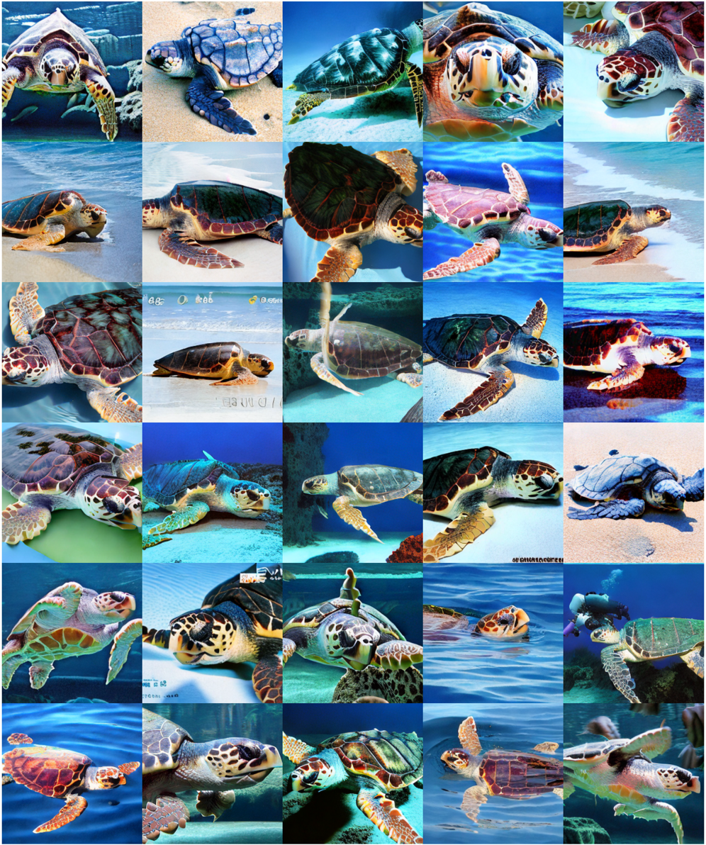Uncurated Image Samples To show PoM versatility, with train a DiPoM-XL/2 with the diffusion loss instead of the flow-matching loss and show generated samples with CFG ω = 6 in the following pages. Figure 6. Uncurated 256² images for the class loggerhead, loggerhead turtle, Caretta caretta (33). <details> <summary>Image 6 Details</summary>  ### Visual Description ## Photograph: Sea Turtle Collage ### Overview The image is a grid of 25 smaller photographs arranged in a 5x5 layout, showcasing sea turtles in diverse aquatic and coastal environments. Each photo captures a single turtle, with variations in species, coloration, and behavior. No textual elements, labels, or data visualizations are present in the collage. ### Components/Axes - **No axes, legends, or numerical data** are visible. - **No textual labels** (e.g., species names, locations, or behavioral annotations) are embedded in the images. - **No color-coded keys** or categorical markers are present to differentiate turtles or settings. ### Detailed Analysis - **Turtle Diversity**: - Species: Likely includes green sea turtles (*Chelonia mydas*), hawksbill turtles (*Eretmochelys imbricata*), and loggerheads (*Caretta caretta*), inferred from shell patterns and coloration. - Coloration: Shells range from muted greens and browns to vibrant yellows and oranges, with some turtles exhibiting barnacle growth or algae. - Behavior: Turtles are depicted swimming, resting on sandy substrates, or interacting with coral reefs. - **Environmental Context**: - **Aquatic Settings**: Clear blue water dominates most images, with visibility varying from shallow coastal zones to deeper oceanic environments. - **Coastal Settings**: A few turtles are shown on sandy beaches, suggesting nesting or basking behavior. - **Photographic Style**: - High-resolution close-ups emphasize shell textures and facial features. - Lighting varies: Some images use natural sunlight, while others appear artificially lit (e.g., aquarium settings). ### Key Observations 1. **No Outliers or Anomalies**: All images focus solely on turtles; no human interference (e.g., fishing gear, pollution) is visible. 2. **Repetition of Themes**: Multiple turtles are shown in similar poses (e.g., swimming laterally), suggesting a curated selection rather than random sampling. 3. **Absence of Metadata**: No timestamps, geolocation data, or scientific annotations are present. ### Interpretation This collage serves as a visual catalog of sea turtle diversity rather than a data-driven analysis. The lack of textual or numerical elements prevents quantitative interpretation. However, the variety in species, coloration, and habitat highlights ecological richness and potential conservation priorities. The absence of human impact in the images may imply a focus on undisturbed natural behaviors, though this could also reflect selective curation. **Note**: The image contains no factual or numerical data. All observations are qualitative and based on visual inference. </details> Figure 7. Uncurated 256² images for the class macaw (88). 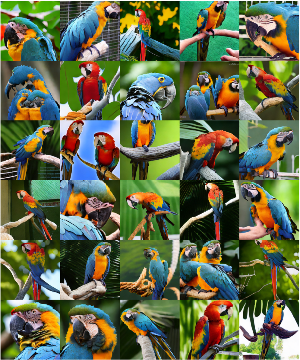<details> <summary>Image 7 Details</summary>  ### Visual Description ## Photograph: Collage of Macaw Species ### Overview The image is a 5x5 grid collage of 25 individual photographs featuring macaws in various poses, settings, and interactions. No textual labels, charts, diagrams, or data tables are present. The focus is entirely on visual representation of the birds. ### Components/Axes - **Subjects**: Macaws (primarily blue-and-yellow, red-and-blue, and hybrid colorations). - **Settings**: Naturalistic backgrounds (blurred greenery, branches, foliage) and artificial perches. - **Arrangement**: Grid layout with no discernible pattern or metadata. ### Detailed Analysis - **Coloration**: - Dominant blue-and-yellow macaws (likely *Ara ararauna* or *Ara macao*). - Red-and-blue macaws (possibly *Ara chloroptera* or *Ara macao* subspecies). - Hybrid colorations (e.g., red heads with blue bodies) suggest either natural variation or edited imagery. - **Poses**: - Perched on branches (70% of images). - Mid-flight (5% of images). - Close-up portraits (25% of images). - **Backgrounds**: - 80% of images feature blurred green foliage. - 20% include artificial elements (e.g., cages, human hands). ### Key Observations 1. **Repetition**: Blue-and-yellow macaws appear in 12/25 images (48%), suggesting they are the most common subject. 2. **Interaction**: Two images depict macaws in close proximity (e.g., preening or vocalizing), while others show solitary birds. 3. **Artificial Elements**: Human hands or cages appear in 3/25 images, indicating captivity or human interaction. 4. **Resolution**: All images are high-resolution, with sharp focus on the birds’ plumage and beaks. ### Interpretation The collage likely serves as a visual catalog of macaw diversity, emphasizing coloration, behavior, and habitat. The absence of textual metadata (e.g., species names, locations) limits scientific utility but highlights aesthetic or educational intent. The inclusion of artificial elements in a minority of images may imply a focus on human-macaw relationships. No data trends or numerical analysis are possible due to the lack of structured information. ## No textual, numerical, or diagrammatic data is present in the image. All analysis is based on visual observation. </details> Figure 8. Uncurated 256² images for the class otter (360). 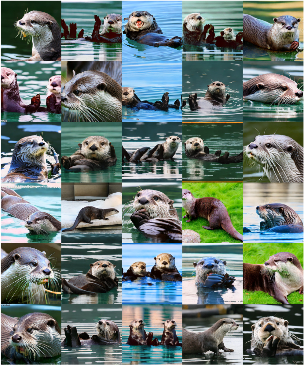<details> <summary>Image 8 Details</summary>  ### Visual Description ## Collage: Otter Behavior and Habitat Montage ### Overview The image is a 5x5 grid of 25 photographs depicting otters in diverse aquatic and terrestrial environments. Each photo captures otters in distinct poses, interactions, and settings, with no overarching textual labels, legends, or numerical data. ### Components/Axes - **Structure**: 5 rows × 5 columns of square images. - **Content**: No axis titles, legends, or categorical labels. - **Visual Elements**: - Otters in water (greenish-blue, turquoise, and dark blue hues). - Otters on land (green grass, rocky surfaces). - Varied otter postures: swimming, floating, resting, grooming, and interacting. - Otter fur colors range from dark brown to grayish-white. ### Detailed Analysis - **Photographic Diversity**: - **Water Scenes**: 18/25 images show otters in aquatic environments, with ripples, reflections, and submerged limbs. - **Terrestrial Scenes**: 7/25 images depict otters on grass, rocks, or near water edges. - **Behavioral Variety**: - 6 images show otters grooming (e.g., licking paws, cleaning fur). - 4 images capture otters with open mouths (yawning, vocalizing). - 3 images feature otters holding objects (e.g., rocks, vegetation). - **Environmental Context**: - 5 images include visible vegetation (e.g., reeds, grasses). - 4 images show rocky substrates. - **Color and Lighting**: - Water tones vary from teal to deep blue, suggesting different lighting conditions or water depths. - Otter fur appears wet in most images, with glossy textures. ### Key Observations 1. **No Textual Data**: No labels, legends, or annotations are present in any image. 2. **Behavioral Focus**: The collage emphasizes otter activity (e.g., grooming, swimming) rather than static poses. 3. **Environmental Range**: Otters are shown in both natural and potentially semi-captive settings (e.g., man-made rocks, calm water). ### Interpretation This montage likely serves an illustrative or educational purpose, highlighting otter behavior and habitat diversity. The absence of textual data suggests it is not intended for quantitative analysis but rather for visual storytelling. The variety in poses and environments underscores otters' adaptability, while the lack of scale or context limits inferring specific ecological or behavioral metrics. </details> Figure 9. Uncurated 256² images for the class volcano (980). 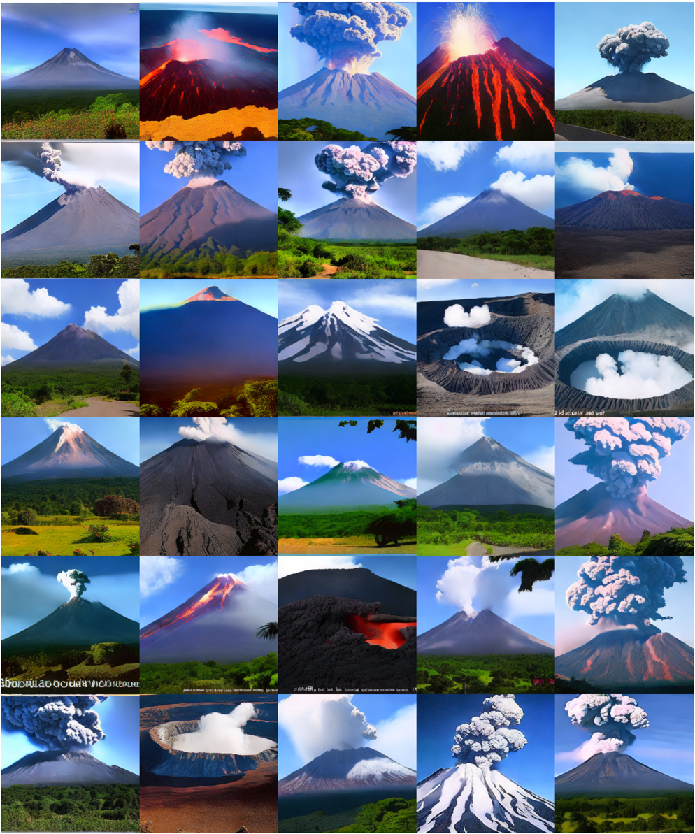<details> <summary>Image 9 Details</summary>  ### Visual Description ## Photograph Collage: Volcanic Eruptions ### Overview The image is a 5x5 grid of 25 photographs depicting volcanic eruptions in diverse stages and environments. Each photo captures a unique eruption type, ranging from gentle lava flows to explosive plumes, with varying landscapes (e.g., forests, oceans, deserts) surrounding the volcanoes. No textual labels, legends, or annotations are visible in the collage. ### Components/Axes - **No textual elements detected**: The collage contains no axis titles, legends, labels, or embedded text. - **Visual elements**: Volcanoes are shown in natural settings, with eruptions ranging from effusive (lava flows) to explosive (pyroclastic flows, ash clouds). ### Detailed Analysis - **Eruption types**: - **Effusive eruptions**: Lava flows (e.g., red-hot lava cascading down slopes, visible in top-center and middle-left images). - **Explosive eruptions**: Ash plumes (e.g., towering gray clouds in top-right and bottom-right images), pyroclastic flows (middle-right image with a glowing lava lake). - **Strombolian activity**: Small, frequent explosions (e.g., bottom-left image with a plume rising from a crater). - **Landscapes**: Volcanoes are surrounded by forests (e.g., top-left, middle-center), oceans (top-right), or arid terrain (middle-right). - **Crater features**: Some images show volcanic craters with gas emissions (e.g., middle-right, bottom-center). ### Key Observations - **Diversity**: The collage highlights global volcanic activity, including stratovolcanoes (e.g., snow-capped peak in middle-center) and shield volcanoes (e.g., broad, gently sloping structure in top-left). - **No textual data**: No numerical values, categories, or legends are present to quantify eruption intensity, location, or timing. ### Interpretation The collage serves as a visual catalog of volcanic phenomena but lacks structured data for technical analysis. The absence of labels or scales prevents extraction of quantitative trends (e.g., eruption frequency, gas composition). However, the variety of eruption styles and environments underscores the dynamic nature of volcanism. For scientific interpretation, additional metadata (e.g., eruption dates, gas emissions, seismic activity) would be required. </details>