2604.06695v1

# Reasoning Fails Where Step Flow Breaks ## Abstract Large reasoning models (LRMs) that generate long chains of thought now perform well on multi-step math, science, and coding tasks. However, their behavior is still unstable and hard to interpret, and existing analysis tools struggle with such long, structured reasoning traces. We introduce Step-Saliency, which pools attention–gradient scores into step-to-step maps along the question–thinking–summary trajectory. Across several models, Step-Saliency reveals two recurring information-flow failures: Shallow Lock-in, where shallow layers over-focus on the current step and barely use earlier context, and Deep Decay, where deep layers gradually lose saliency on the thinking segment and the summary increasingly attends to itself and the last few steps. Motivated by these patterns, we propose StepFlow, a saliency-inspired test-time intervention that adjusts shallow saliency patterns measured by Step-Saliency via Odds-Equal Bridge and adds a small step-level residual in deep layers via Step Momentum Injection. StepFlow improves accuracy on math, science, and coding tasks across multiple LRMs without retraining, indicating that repairing information flow can recover part of their missing reasoning performance. Code is available at https://github.com/XiaoyuXu-Vincent/step-saliency. footnotetext: † Corresponding author, ‡ Project leader Reasoning Fails Where Step Flow Breaks Xiaoyu Xu 1,2, Yulan Pan 2, Xiaosong Yuan 3 ‡, Zhihong Shen 2, Minghao Su 2, Yuanhao Su 2, Xiaofeng Zhang 1 † 1 Shanghai Jiao Tong University, 2 Fuzhou University, 3 Jilin University framebreak@sjtu.edu.cn ## 1 Introduction Large reasoning models (LRMs) generate an internal thinking segment before producing a final summary, forming a question–thinking–summary trajectory. These models achieve strong performance on multi-step mathematics, code generation, and scientific question answering Ahn et al. (2024); Plaat et al. (2025); Xu et al. (2025). Despite these gains, LRMs still exhibit persistent failure modes, including unfaithful chains of thought Paul et al. (2024); Lightman et al. (2023); Barez et al. (2025), overconfident hallucinations Fan et al. (2025); Cao et al. (2025), and brittleness on compositional tasks Song et al. (2025); Li et al. (2025c); Boye and Moell (2025); Simhi et al. ; Chen et al. (2025b). When an LRM makes a mistake, we lack a clear way to attribute the final error to the model’s internal reasoning trace. This motivates a diagnostic that tracks step-to-step influence across depth and links shifts in that influence to incorrect final answers Luo and Specia (2024); Cambria et al. (2024); Yang et al. . 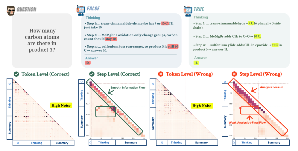Prior work offers several token-level diagnostics for inspecting LRMs during generation. Attention-based analyses visualize which tokens receive attention when producing later tokens Vig and Belinkov (2019); Yeh et al. (2023), but attention weights are not always faithful indicators of what actually drives the prediction Jain and Wallace (2019). Saliency-based methods instead assign gradient-weighted importance to earlier tokens Ancona et al. (2017); Wu et al. (2023), yet along long reasoning traces the scores can be noisy and difficult to aggregate across positions. The main difficulty is not the lack of signals but the lack of a readable unit aligned with reasoning steps: token-level maps are dense, local, and do not naturally summarize step-to-step dependence. As Figure 1 shows, even when correct and error traces differ, the signal is dispersed across many tokens, making it difficult to summarize which steps remain influential later and how this changes with depth. <details> <summary>2604.06695v1/x1.png Details</summary>  ### Visual Description ## Heatmap Visualization: Token-Level vs Step-Level Analysis of Chemical Problem Solving ### Overview The image presents a comparative analysis of two solution paths (False and True) to a chemistry problem about carbon atom counting in a chemical product. It includes four heatmaps visualizing the relationship between "Thinking" and "Summary" components at both token-level and step-level analysis, with color-coded correctness indicators. ### Components/Axes **Heatmap Structure:** - **X-axis (Horizontal):** "Thinking" component (0-150 scale) - **Y-axis (Vertical):** "Summary" component (0-150 scale) - **Legend:** - Green = Correct analysis - Red = Incorrect analysis - **Annotations:** - "High Noise" labels - Arrows indicating information flow/analysis lock-in - Text boxes highlighting key steps **Spatial Positioning:** - Top-left: Question box with chemistry problem - Middle: Two solution paths (False/True) with step-by-step reasoning - Bottom: Four heatmaps arranged in 2x2 grid: - Top-left: Token Level (Correct) - Top-right: Token Level (Wrong) - Bottom-left: Step Level (Correct) - Bottom-right: Step Level (Wrong) ### Detailed Analysis **Token Level Heatmaps:** 1. **Correct (Green):** - Diagonal green band from (0,0) to (150,150) - Indicates strong correlation between thinking and summary components - "High Noise" annotation in bottom-right quadrant 2. **Incorrect (Red):** - Red band concentrated in bottom-left quadrant - "High Noise" annotation in top-right quadrant - Weak diagonal correlation compared to correct version **Step Level Heatmaps:** 1. **Correct (Green):** - Smooth green gradient from top-left to bottom-right - Clear information flow from thinking to summary - No noise annotations 2. **Incorrect (Red):** - Red band with "Analysis Lock-in" annotation - Steeper diagonal than correct version - Weak final flow indicated by red arrow ### Key Observations 1. Token-level analysis shows higher noise in incorrect solutions 2. Step-level correct solutions demonstrate smoother information flow 3. Incorrect step-level analysis exhibits "lock-in" effects 4. Correct solutions maintain stronger thinking-summary correlation 5. Noise patterns differ between token and step-level evaluations ### Interpretation The visualization demonstrates that step-level analysis provides more reliable chemical problem-solving than token-level analysis. The "Analysis Lock-in" phenomenon in incorrect step-level solutions suggests cognitive biases persisting through reasoning steps. The "High Noise" annotations in token-level incorrect solutions indicate greater variability in surface-level processing errors. The smooth information flow in correct step-level solutions aligns with the True solution path's systematic approach to molecular counting, while the False path's abrupt carbon count change (10→11) correlates with the analysis lock-in pattern. This supports the conclusion that structured reasoning steps outperform superficial token analysis in complex chemical calculations. </details> Figure 1: From token- to step-level saliency. Token-level saliency maps are dense and noisy; Step-Saliency pools them into question/thinking/summary blocks. Correct traces show smooth question $→$ thinking $→$ summary flow, while errors exhibit shallow lock-in and weak thinking $→$ summary links. 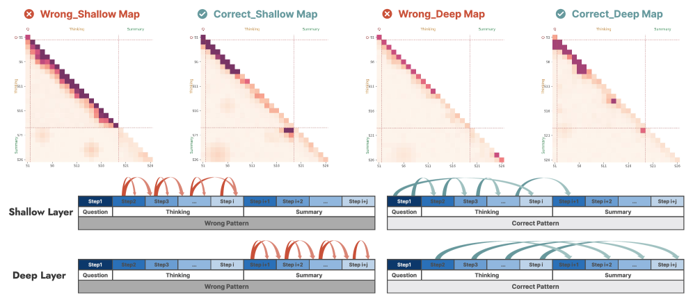To address this limitation, we introduce Step-Saliency, a step-level diagnostic for long-form reasoning. We compute token saliency using attention–gradient influence and then pool the scores within each step. This yields a compact step $→$ step map that is easy to compare across layers. Applying Step-Saliency to several LRMs, we observe two common patterns in incorrect outputs. In shallow layers, influence concentrates on the current thinking step and its immediate neighbors, while earlier context is suppressed; we call this Shallow Lock-in. As depth increases, saliency on the thinking segment weakens for both correct and incorrect outputs, but it fades much faster on incorrect ones, and the summary becomes more self-focused; we call this Deep Decay (§ 3.2). Building on these observations, we propose StepFlow, a lightweight test-time intervention that modifies a model’s forward pass without retraining or backpropagation. StepFlow has two components that target the two failure patterns. Odds-Equal Bridge (OEB) is applied to the first few layers: when the model is generating a thinking step, it prevents step-level mass from collapsing onto the just-written tokens by keeping a non-trivial share on the question and earlier steps. Step Momentum Injection (SMI) is applied to the last few layers: at step boundaries, it carries a small residual summary of the previous step into the next step, so earlier reasoning remains available when the summary is produced. Together, OEB and SMI promote a steadier question–thinking–summary linkage during generation. We evaluate StepFlow on DeepSeek-R1-Distill (7B/14B/32B), GPT-OSS-20B, and QwQ-32B-Preview across six benchmarks: AIME24, AIME25, AMC23, MATH-500, GPQA-Diamond, and LiveCodeBench. StepFlow consistently improves accuracy across all backbones, with the largest gains on competition-style problems that require long reasoning chains. Our main contributions are as follows: - We introduce Step-Saliency, a diagnostic that aggregates token-level saliency into step $→$ step maps, making long reasoning traces interpretable at the step level. - We identify two depth-wise information-flow failure patterns in large reasoning models, which we term Shallow Lock-in and Deep Decay; they reliably separate incorrect from correct traces in our saliency analysis. - We propose StepFlow, a test-time intervention that reshapes information flow via Odds-Equal Bridge and Step Momentum Injection, improving accuracy across multiple benchmarks without retraining. <details> <summary>2604.06695v1/x2.png Details</summary>  ### Visual Description ## Heatmaps and Process Flow Diagrams: Shallow vs. Deep Layer Analysis ### Overview The image presents four heatmaps and two process flow diagrams comparing "Shallow Layer" and "Deep Layer" patterns. The heatmaps visualize data distributions across "Thinking" and "Summary" axes, while the diagrams illustrate step-by-step workflows with directional arrows. Key distinctions are marked with ✅ (Correct) and ❌ (Wrong) labels. --- ### Components/Axes #### Heatmaps - **Axes**: - **X-axis (Thinking)**: Labeled with values `S1` to `S24` (e.g., `S1`, `S6`, `S11`, `S16`, `S21`, `S24`). - **Y-axis (Summary)**: Labeled with values `Q` to `S26` (e.g., `Q`, `S1`, `S11`, `S16`, `S21`, `S26`). - **Legend**: - **Red**: High-intensity data points (dark red to light red gradient). - **Green**: Checkmark (✅) for Correct patterns; ❌ for Wrong patterns. - **Placement**: - Heatmaps occupy the top half of the image, arranged left-to-right: `Wrong_Shallow`, `Correct_Shallow`, `Wrong_Deep`, `Correct_Deep`. #### Process Flow Diagrams - **Components**: - **Steps**: Labeled `Step1` to `Step i+j` (e.g., `Step1`, `Step2`, `Step3`, `...`, `Step i`, `Step i+1`, `Step i+2`). - **Sections**: - **Thinking**: Gray background with steps in blue. - **Summary**: Gray background with steps in darker blue. - **Arrows**: - **Red**: Indicate cyclic/incorrect patterns (Wrong). - **Green**: Indicate linear/correct patterns (Correct). - **Placement**: - Diagrams are positioned below the heatmaps, split into "Shallow Layer" (left) and "Deep Layer" (right). --- ### Detailed Analysis #### Heatmaps 1. **Wrong_Shallow**: - Dense red shading in the top-left quadrant (high "Thinking," low "Summary"). - Gradual fading toward the bottom-right (lower "Thinking," higher "Summary"). 2. **Correct_Shallow**: - Concentrated red shading in the mid-range of both axes (balanced "Thinking" and "Summary"). - A distinct cluster near `S11` (X-axis) and `S16` (Y-axis). 3. **Wrong_Deep**: - Similar to Wrong_Shallow but with a broader spread across the top-right quadrant. 4. **Correct_Deep**: - High-intensity red shading in the bottom-right quadrant (low "Thinking," high "Summary"). - A single prominent data point near `S24` (X-axis) and `S26` (Y-axis). #### Process Flow Diagrams 1. **Shallow Layer**: - **Wrong Pattern**: Red arrows loop between `Step1` and `Step i+1`, creating a cyclical flow. - **Correct Pattern**: Green arrows progress linearly from `Step1` to `Step i+j` without loops. 2. **Deep Layer**: - **Wrong Pattern**: Red arrows form a tighter loop between `Step1` and `Step i+2`. - **Correct Pattern**: Green arrows follow a linear path from `Step1` to `Step i+j`, with broader spacing between steps. --- ### Key Observations 1. **Heatmap Trends**: - Correct patterns (Shallow/Deep) show more focused data distributions compared to Wrong patterns. - Correct_Deep exhibits the most extreme divergence, with data concentrated in the lowest "Thinking" and highest "Summary" range. 2. **Diagram Flow**: - Correct patterns (green arrows) emphasize linear progression, while Wrong patterns (red arrows) highlight inefficiency through cyclical loops. - Deep Layer diagrams show more complex step interactions than Shallow Layer. --- ### Interpretation 1. **Data Implications**: - The heatmaps suggest that Correct patterns optimize resource allocation: - **Correct_Shallow** balances "Thinking" and "Summary" efforts. - **Correct_Deep** minimizes "Thinking" while maximizing "Summary" efficiency. - Wrong patterns indicate wasted effort, with data spread across less productive ranges. 2. **Process Flow Insights**: - The diagrams reinforce the heatmap findings: linear workflows (Correct) avoid redundant steps, while cyclical loops (Wrong) suggest inefficiency. - The Deep Layer’s tighter loops in Wrong patterns may reflect overcomplication, whereas Correct patterns prioritize streamlined execution. 3. **Anomalies**: - The single data point in Correct_Deep’s bottom-right quadrant (near `S24`/`S26`) could represent an outlier or a critical high-efficiency case. - The absence of data in the top-right quadrant of Correct_Shallow may indicate a design constraint or intentional focus on mid-range values. --- ### Conclusion The image demonstrates that Correct patterns—both Shallow and Deep—achieve better performance by concentrating efforts in optimal ranges ("Thinking" vs. "Summary"). The process flow diagrams visually validate this, showing linear progression as a hallmark of efficiency. The use of color (red for errors, green for correctness) and spatial arrangement (heatmaps above diagrams) creates a cohesive narrative linking data distribution to workflow design. </details> Figure 2: Step-Saliency patterns for shallow vs. deep layers and correct vs. error traces. Top: depth-collapsed step $→$ step saliency maps; darker red indicates stronger influence between steps. Bottom: schematic diagrams summarizing the observed patterns—red arrows denote narrow, local flow (Shallow Lock-in and Deep Decay in error traces), while blue arrows denote broad, long-range flow in correct traces. ## 2 Related Work ### 2.1 Large Reasoning Models Chain-of-thought prompting (CoT) Wei et al. (2022) substantially improved LLM reasoning and spurred Large Reasoning Models (LRMs) with strong multi-step reasoning and structured intermediate traces. Although LRMs demonstrate strong performance on multi-step reasoning benchmarks Kojima et al. (2022); Chen et al. (2025a); Xu et al. (2025); Lanham et al. (2023), their reasoning processes still suffer from instability and limited interpretability. Beyond standard CoT prompting, test-time scaling methods such as self-consistency and sampled-path selection improve robustness Wang et al. (2023b); Muennighoff et al. (2025). Other work builds multi-step frameworks with tools or self-improvement Li et al. (2025b, 2023); Yuan et al. (2024); Dutta et al. (2024). Our understanding of how information is propagated, transformed, and possibly lost inside LRMs remains incomplete, which makes it difficult to systematically analyze reasoning failures, incorrect inferences, and inconsistent answers Song et al. (2025); Li et al. (2025c); Chen et al. (2025b). ### 2.2 Layer-wise Reasoning Behavior Many studies employing layer-wise analysis have revealed that Transformer-based LLMs exhibit a clear functional division across network depth during reasoning Geva et al. (2021). In the shallow layers, the model primarily performs local and formal pattern recognition, such as extracting n-gram features Sajjad et al. (2022); Vulić et al. (2020) and handling structural information Van Aken et al. (2019). In the deep layers, the model shifts toward cross-sentence and cross-concept integration, handling semantic alignment Saglam et al. (2025), long-range dependency modeling Wang et al. (2020b), and the global organization of the reasoning chain Dong et al. (2023). ### 2.3 Information Flow To study how information moves inside LLMs, prior work has proposed a range of information-flow analyses Zhao et al. (2024); Luo and Specia (2024); Cambria et al. (2024). Attention-based methods inspect attention weights or head activations Vig and Belinkov (2019); Yeh et al. (2023) to show which tokens the model focuses on. They are often used to infer context-dependency structures Vashishth et al. (2019). However, attention is not a faithful explanation: different attention maps can lead to the same prediction Jain and Wallace (2019). Kobayashi et al. Kobayashi et al. (2020) therefore separate the contribution of attention weights from that of transformed value vectors, partially decoupling "where the model looks" from "what representation is propagated". Yan et al. Yan et al. (2025) propose attention-level interventions to better preserve CoT context, complementary to saliency-based analyses. Saliency-based methods instead assign importance scores to tokens using gradient-based, perturbation-based, or gradient–activation techniques Ancona et al. (2017); Huber et al. (2022); Ding and Koehn (2021); Boggust et al. (2023). These scores highlight which tokens support answers or intermediate reasoning steps Wang et al. (2020a); Dong et al. (2023); Wu et al. (2023); Lee and Hockenmaier (2025) and are more tightly coupled to the model’s actual computation than raw attention. Yet they are typically local to a single prediction and often noisy, which makes it difficult to obtain stable, sequence-level explanations of how information flows through a long reasoning trace. ## 3 Motivation and Information Flow Analysis ### 3.1 Saliency and step-level aggregation #### Saliency (token $→$ token). Let $x_1:T$ be the generated tokens and $L_t=-\log p_θ(x_t\mid x_<t)$ the token-level loss. For layer $\ell$ and head $h$ , let $A^(\ell,h)∈ℝ^T× T$ denote the causal attention matrix. For each query position $t$ and key position $k≤ t$ , we compute the gradient-weighted influence and average over $H$ heads: $$ I^(\ell)_t← k = \frac{1}{H}∑_h=1^H\Bigl| A^(\ell,h)_t,k·\frac{∂L_t}{∂ A^(\ell,h)_t,k} \Bigr|, k≤ t. \tag{1} $$ We take absolute values to measure influence magnitude regardless of direction; signed scores would complicate step-level aggregation in Eq. (3) since positive and negative contributions could cancel within a step. Signed influence could reveal suppression patterns but would require separate positive/negative pooling, which we leave for future work. Stacking over all $t$ gives the full influence matrix $I^(\ell)∈ℝ^T× T$ . We then apply per-query row normalization to obtain a token $→$ token saliency distribution: $$ \tilde{s}^(\ell)_t← k = \frac{\bigl(I^(\ell)\bigr)_t← k}{∑_k^\prime≤ t\bigl(I^(\ell)\bigr)_t← k^\prime+ε} . \tag{2} $$ Compared with raw attention, these scores reflect how much each past token contributes to the loss at position $t$ and remain informative even when attention is diffuse (full computation details in Appendix A.1). #### From tokens to steps. For each generation trace, we segment the sequence into a question segment, a multi-step thinking segment, and a summary segment. Let $Γ_1,\dots,Γ_K$ denote the $K$ thinking steps (each $Γ_i$ is a contiguous token span) and $Γ_K+1$ the summary segment; we use $Γ_i$ generically to refer to any segment when the context is clear. For layer $\ell$ , we aggregate token-level saliency into step $→$ step blocks: $$ M^(\ell)_j← i = \frac{1}{|Γ_j| |Γ_i|}∑_t∈Γ_{j}∑_k∈Γ_{i}\tilde{s}^(\ell)_t← k, i≤ j . \tag{3} $$ We use mean pooling to suppress token-level noise (cf. Figure 1); the trade-off is some loss of fine-grained signal. Mass on the block diagonal captures within-segment self-reinforcement; off-diagonal mass captures cross-step and cross-segment flow. Averaging $M^(\ell)$ over layers yields a depth-collapsed step $→$ step map (i.e., averaged over depth), which we refer to as the Step-Saliency map. ### 3.2 Information flow among steps We compare correct and error traces for identical prompts using layerwise Step-Saliency maps (Figure 2). Each map summarizes how strongly a given thinking step or the summary depends on earlier steps across depth. #### Shallow layers: Shallow Lock-in. In shallow layers, correct traces keep a visible link to the question and spread saliency across several thinking steps. The model continues to refer back to the problem statement and to earlier parts of its reasoning. Error traces instead place most saliency inside a narrow band around the current step and its immediate neighbors, while saliency on the question and early thinking steps is strongly suppressed. The model attends mainly to what it just wrote. We refer to this local feedback pattern as Shallow Lock-in. #### Deep layers: Deep Decay. In deeper layers, saliency on the thinking segment decreases for both correct and error traces, but the decay is faster for errors. For correct traces, summary tokens still allocate noticeable saliency back to several earlier thinking steps, indicating that the answer remains connected to the internal reasoning. For error traces, deep layers place most saliency on summary tokens themselves and on the last few thinking steps, with very little mass on earlier steps. We call this faster loss of thinking saliency in deep layers Deep Decay: the summary is produced with only a thin connection to the full reasoning chain. ### 3.3 Quantifying inter-step flow To summarize these map-level patterns, we define two simple layerwise metrics based on the Step-Saliency blocks. #### Definitions. Let $M^(\ell)_j← i$ be the step $→$ step map at layer $\ell$ from Eq. (3). We summarize within-thinking and within-summary self-reinforcement as $$ I^(\ell)_T=\frac{1}{K}∑_i=1^KM^(\ell)_i← i and I^(\ell)_S=M^(\ell)_(K+1)←(K+1), \tag{4} $$ where $I^(\ell)_T$ measures how much each step reuses its own content and $I^(\ell)_S$ measures how much the summary attends to itself across depth. 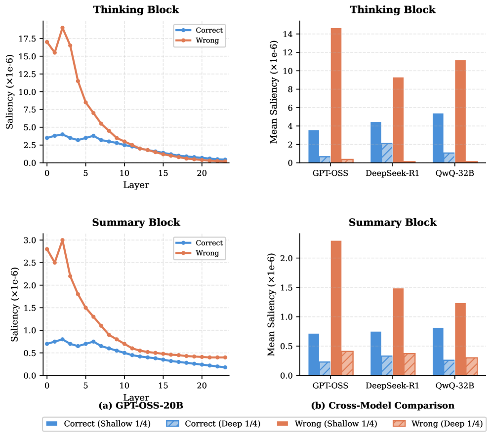Figure 3 shows that, for error traces, thinking self-intensity is higher in shallow layers and decreases faster with depth, while summary self-saliency rises earlier and becomes more self-focused in deep layers, with much weaker connections back to earlier thinking steps than in correct traces. <details> <summary>2604.06695v1/x3.png Details</summary>  ### Visual Description ## Line Graphs: Thinking Block Saliency Across Layers ### Overview Two line graphs compare saliency values (x1e-6) across layers (0-20) for "Correct" and "Wrong" predictions in a "Thinking Block" architecture. The left graph shows data for GPT-OSS-20B, while the right graph compares cross-model performance (GPT-OSS, DeepSeek-R1, QwQ-32B). ### Components/Axes - **X-axis**: Layer (0-20) - **Y-axis**: Saliency (x1e-6) - **Legends**: - **Blue (solid)**: Correct predictions - **Red (dashed)**: Wrong predictions ### Detailed Analysis #### Left Graph (GPT-OSS-20B): - **Correct (blue)**: - Starts at ~3.5e-6 (layer 0), peaks at ~4.5e-6 (layer 2), then declines steadily to ~0.5e-6 (layer 20). - Trend: Gradual decay after layer 2. - **Wrong (red)**: - Starts at ~16e-6 (layer 0), spikes to ~18e-6 (layer 2), then drops sharply to ~1e-6 (layer 20). - Trend: Steep decline after layer 2. #### Right Graph (Cross-Model Comparison): - **Mean Saliency (x1e-6)**: - **GPT-OSS**: - Correct: ~3.5e-6 - Wrong: ~14e-6 - **DeepSeek-R1**: - Correct: ~4.2e-6 - Wrong: ~9e-6 - **QwQ-32B**: - Correct: ~5e-6 - Wrong: ~11e-6 ### Key Observations 1. **Layer Dependency**: Saliency for both Correct and Wrong predictions decreases significantly with deeper layers in GPT-OSS-20B. 2. **Model Performance**: - GPT-OSS has the highest Wrong saliency (14e-6) and lowest Correct saliency (3.5e-6). - QwQ-32B shows the highest Correct saliency (5e-6) but still high Wrong saliency (11e-6). 3. **Anomaly**: The red (Wrong) line in GPT-OSS-20B spikes at layer 2 before declining, suggesting a transient error pattern. ### Interpretation - **Thinking Block Dynamics**: The sharp decline in Wrong saliency after layer 2 in GPT-OSS-20B implies that deeper layers may suppress erroneous predictions, though Correct saliency remains low overall. - **Model Comparison**: Cross-model data reveals a trade-off between Correct and Wrong saliency. QwQ-32B balances higher Correct saliency with moderate Wrong saliency, suggesting better error handling than GPT-OSS. - **Practical Implication**: Models with higher Correct saliency (e.g., QwQ-32B) may prioritize relevant features, while lower Wrong saliency indicates reduced reliance on misleading patterns. ## Bar Charts: Summary Block Saliency ### Overview Two bar charts compare mean saliency (x1e-6) for "Correct" and "Wrong" predictions in a "Summary Block" across three models: GPT-OSS, DeepSeek-R1, and QwQ-32B. ### Components/Axes - **X-axis**: Models (GPT-OSS, DeepSeek-R1, QwQ-32B) - **Y-axis**: Mean Saliency (x1e-6) - **Legends**: - **Blue (solid)**: Correct predictions - **Red (striped)**: Wrong predictions ### Detailed Analysis #### Left Chart (GPT-OSS-20B): - **Correct (blue)**: ~0.7e-6 - **Wrong (red)**: ~0.4e-6 #### Right Chart (Cross-Model Comparison): - **GPT-OSS**: - Correct: ~0.7e-6 - Wrong: ~0.4e-6 - **DeepSeek-R1**: - Correct: ~0.8e-6 - Wrong: ~0.3e-6 - **QwQ-32B**: - Correct: ~0.9e-6 - Wrong: ~0.2e-6 ### Key Observations 1. **Model Consistency**: All models show higher Correct saliency than Wrong saliency in the Summary Block. 2. **QwQ-32B Advantage**: Highest Correct saliency (0.9e-6) and lowest Wrong saliency (0.2e-6), indicating superior summarization accuracy. 3. **GPT-OSS Limitation**: Lowest Correct saliency (0.7e-6) and moderate Wrong saliency (0.4e-6), suggesting weaker summarization performance. ### Interpretation - **Summary Block Efficiency**: The Summary Block amplifies Correct saliency while suppressing Wrong saliency compared to the Thinking Block. - **Model Hierarchy**: QwQ-32B outperforms others in leveraging relevant features (high Correct) and ignoring irrelevant ones (low Wrong). - **Cross-Block Comparison**: The Thinking Block’s higher saliency values (e.g., 14e-6 Wrong in GPT-OSS) suggest it is more sensitive to errors, while the Summary Block refines predictions. ## Final Synthesis The data demonstrates that deeper layers in the Thinking Block reduce saliency for both Correct and Wrong predictions, with QwQ-32B showing the most balanced performance. The Summary Block further refines this by prioritizing Correct saliency, highlighting QwQ-32B’s superiority in handling summarization tasks. These trends underscore the importance of layer depth and model architecture in balancing accuracy and error mitigation. </details> Figure 3: Layer-wise saliency intensities across three models. (a) GPT-OSS-20B: thinking and summary self-intensities for correct vs. error traces. (b) R1-Distill-32B and QwQ-32B show the same pattern: stronger shallow lock-in and summary self-reinforcement in error traces. Across models, error traces show higher shallow thinking self-intensity and earlier/higher summary self-intensity, consistent with Shallow Lock-in and Deep Decay. ## 4 Method Guided by the Step-Saliency patterns in § 3.3, we design StepFlow, a test-time intervention with two components: Odds-Equal Bridge (OEB) for shallow layers and Step Momentum Injection (SMI) for deep layers. ### 4.1 Odds-Equal Bridge (OEB) OEB aims to avoid a situation where almost all influence mass sits on the current thinking step and its neighbours, while earlier context is ignored. #### Group-wise proxy target. For a fixed query position $t$ in one head and one layer, let $p_t$ be the causal attention distribution over past tokens for this head. Step-Saliency uses attention–gradient products for offline diagnosis, while OEB uses $p_t$ as a lightweight proxy during decoding to enforce a minimum mass on the bridge region. Using the segmentation from Step-Saliency, we split the keys into three disjoint sets: the current segment $S$ , a bridge segment $B$ that represents earlier context we want to preserve (e.g., the question while generating analysis, or the analysis while generating the summary), and all remaining tokens $O$ . We define the current group masses $$ p_t(g)=∑_k∈ gp_t(k), g∈\{S,B,O\}. \tag{5} $$ We keep $p_t(O)$ fixed and set a soft lower bound on the bridge mass: $$ \displaystyleτ_B \displaystyle=\min≤ft(√{\frac{|B|}{|B|+|S|}}, τ_\max\right), \displaystyleτ_S \displaystyle=1-p_t(O)-τ_B. \tag{6} $$ We apply OEB only when the bridge mass falls below the bound, $p_t(B)<τ_B$ ; otherwise we leave the logits unchanged. This schedule keeps the bridge on the same order of magnitude as the current segment instead of letting its mass shrink to nearly zero. Intuitively, the lower bound grows with the relative size of the bridge region, the square-root dampens extreme length effects, and $τ_\max$ caps the intervention so OEB cannot dominate the attention distribution. A single scalar $τ_\max$ is chosen per model; we show in Appendix B.1 that accuracy is robust across a wide range of $τ_\max$ values. #### KL projection on logits. Let $z$ denote the attention logits (before the causal-mask softmax) for query position $t$ in a given layer/head, so that $p_t=softmax(z)$ . When $p_t(B)<τ_B$ , we seek a new distribution $q_t$ that stays as close as possible to $p_t$ in KL divergence while enforcing $q_t(O)=p_t(O)$ and $q_t(B)=τ_B$ , and hence $q_t(S)=τ_S$ . This gives a small projection problem $\arg\min_q_{t}KL(q_t \| p_t)$ under linear constraints on group totals, which can be viewed as a constrained Bregman (KL) projection Banerjee et al. (2005). Under the softmax parameterization, the solution reduces to a simple group-wise shift of the scores: $$ z^\prime_k = z_k+λ_g, k∈ g, g∈\{S,B\}, \tag{7} $$ where, when the constraint is active, $$ λ_B=\log\frac{τ_B}{p_t(B)} and λ_S=\log\frac{τ_S}{p_t(S)}. \tag{8} $$ Scores in $O$ are left unchanged. The group-wise shift in Eq. (7) ensures that when bridge mass falls below the threshold, attention logits are adjusted to maintain a minimum share on the bridge region, preventing the collapse of influence onto the current segment alone. ### 4.2 Step Momentum Injection (SMI) SMI targets deep-layer decay. As depth increases, thinking saliency tends to drift toward background, especially on error traces. SMI treats deep layers as a leaky integrator and nudges them towards a mild accumulator: it preserves a small amount of step-level content while keeping the backbone computation intact. #### Step segmentation. We reuse the step segmentation defined for Step-Saliency: the thinking segment is split into steps $Γ_1,\dots,Γ_K$ , and the summary tokens form a summary segment $Γ_K+1$ . Boundaries are detected using the model’s analysis marker plus simple punctuation and template cues, and StepFlow is empirically robust to small boundary shifts (Appendix A.2). Table 1: Accuracy (%) on six benchmarks (columns) across multiple backbones. | Method | Math / Science | Code | | | | | | --- | --- | --- | --- | --- | --- | --- | | AIME24 | AIME25 | AMC23 | MATH-500 | GPQA-D | LiveCodeBench | | | DeepSeek-R1-Distill-Qwen 7B | 54.0 | 39.2 | 82.5 | 92.8 | 49.1 | 37.6 | | + Budget Forcing (S1) | 56.2 | 39.5 | 84.0 | 93.1 | 51.3 | 39.8 | | + Hint-Infer (Round1) | 57.5 | 43.3 | 85.2 | 93.0 | 56.6 | 45.2 | | + Plan-and-Solve (PS+) | 58.8 | 42.6 | 86.0 | 93.3 | 52.8 | 42.0 | | + Attn-Interv. | 56.5 | 41.0 | 84.5 | 93.0 | 51.8 | 40.5 | | + Act. Steering | 57.0 | 41.5 | 84.8 | 93.1 | 52.0 | 41.2 | | + StepFlow | 62.5 | 43.8 | 88.0 | 93.8 | 57.6 | 47.1 | | DeepSeek-R1-Distill-Qwen 14B | 69.7 | 50.2 | 87.1 | 93.9 | 59.1 | 53.1 | | + Budget Forcing (S1) | 70.5 | 54.8 | 90.0 | 94.1 | 60.2 | 54.8 | | + Hint-Infer (Round1) | 71.2 | 53.0 | 88.5 | 94.1 | 61.0 | 56.2 | | + Plan-and-Solve (PS+) | 71.8 | 54.5 | 89.2 | 94.1 | 61.8 | 57.0 | | + Attn-Interv. | 70.8 | 52.5 | 88.0 | 94.0 | 60.5 | 55.5 | | + Act. Steering | 71.0 | 53.2 | 88.2 | 94.0 | 60.8 | 55.0 | | + StepFlow | 72.1 | 57.7 | 89.7 | 94.2 | 63.1 | 59.9 | | DeepSeek-R1-Distill-Qwen 32B | 72.6 | 54.9 | 93.8 | 94.3 | 62.1 | 57.2 | | + Budget Forcing (S1) | 73.2 | 56.5 | 94.9 | 94.9 | 63.8 | 58.5 | | + Hint-Infer (Round1) | 73.0 | 57.8 | 94.5 | 94.8 | 63.5 | 59.8 | | + Plan-and-Solve (PS+) | 74.0 | 59.5 | 94.9 | 95.0 | 63.8 | 60.5 | | + Attn-Interv. | 73.5 | 57.5 | 94.2 | 94.5 | 62.9 | 59.8 | | + Act. Steering | 74.0 | 58.2 | 94.5 | 94.6 | 64.0 | 58.5 | | + StepFlow | 74.5 | 66.7 | 95.3 | 95.6 | 64.5 | 63.0 | | GPT-OSS-20B low | 41.8 | 39.1 | 83.9 | 86.2 | 57.1 | 52.4 | | + Budget Forcing (S1) | 44.9 | 40.5 | 85.2 | 87.0 | 58.5 | 53.8 | | + Hint-Infer (Round1) | 44.5 | 41.8 | 86.5 | 86.8 | 59.8 | 56.2 | | + Plan-and-Solve (PS+) | 45.6 | 42.8 | 87.2 | 87.5 | 60.8 | 57.0 | | + Attn-Interv. | 43.5 | 40.8 | 85.5 | 86.8 | 58.8 | 55.0 | | + Act. Steering | 44.0 | 41.2 | 85.8 | 87.0 | 59.2 | 55.5 | | + StepFlow | 47.9 | 46.5 | 90.0 | 89.6 | 64.0 | 62.3 | | GPT-OSS-20B medium | 63.4 | 62.0 | 94.2 | 89.2 | 65.2 | 70.0 | | + Budget Forcing (S1) | 65.2 | 63.5 | 94.6 | 89.6 | 66.5 | 72.5 | | + Hint-Infer (Round1) | 65.0 | 64.8 | 94.8 | 89.5 | 67.8 | 74.5 | | + Plan-and-Solve (PS+) | 65.6 | 66.0 | 95.0 | 89.9 | 68.5 | 75.8 | | + Attn-Interv. | 64.8 | 66.2 | 94.5 | 89.5 | 66.0 | 75.8 | | + Act. Steering | 65.5 | 64.5 | 94.6 | 89.6 | 66.8 | 72.5 | | + StepFlow | 66.0 | 69.2 | 95.5 | 90.5 | 70.3 | 79.5 | | QwQ-32B-Preview | 50.0 | 40.0 | 80.0 | 90.6 | 58.1 | 41.4 | | + Budget Forcing (S1) | 54.5 | 41.5 | 82.0 | 91.0 | 59.5 | 46.2 | | + Hint-Infer (Round1) | 52.8 | 42.8 | 83.5 | 90.3 | 60.8 | 44.8 | | + Plan-and-Solve (PS+) | 53.8 | 44.0 | 84.5 | 91.2 | 61.5 | 46.5 | | + Attn-Interv. | 52.0 | 42.2 | 82.5 | 90.8 | 59.8 | 44.5 | | + Act. Steering | 53.0 | 43.5 | 83.0 | 91.0 | 59.2 | 45.0 | | + StepFlow | 57.3 | 48.0 | 91.0 | 92.0 | 63.3 | 50.3 | #### Step-level residual link. At the boundary between $Γ_i$ and $Γ_i+1$ , we build a step-level momentum vector from the deep-layer value states of step $Γ_i$ . In practice, $v_k$ is taken as the multi-head attention value projection output (concatenated over heads) at the selected deep layers. Let $\{v_k\}_k∈Γ_{i}$ be the corresponding value vectors and define a single step summary $$ m_prev=\frac{1}{|Γ_i|}∑_k∈Γ_{i}v_k. \tag{9} $$ We then inject this momentum as a residual into the hidden state of the first token $t$ of $Γ_i+1$ in a subset of deep layers: $$ h^\prime_t=h_t+α m_prev. \tag{10} $$ We add the residual on the layer’s residual stream before the MLP block. The scalar $α$ is a small, fixed coefficient per model; details and implementation variants are given in Appendix B.1. By injecting the momentum vector at step boundaries, SMI maintains a connection from earlier thinking steps to later positions, counteracting the tendency for deep layers to lose saliency on the thinking segment. Algorithm 1 StepFlow single-pass decoding 1: $M, L_sh, L_dp, τ_\max, α$ 2: for $t=1,2,\dots$ do 3: $(S,B,O)←\textsc{PartitionKeys}(t)$ 4: $τ_B←\min\Big(√{\frac{|B|}{|B|+|S|}}, τ_\max\Big)$ 5: for $\ell∈L_sh$ do 6: $p_g←∑_k∈ gsoftmax(z^(\ell)_t)[k] (g∈\{S,B,O\})$ 7: if $p_B<τ_B$ then 8: $τ_S← 1-p_O-τ_B$ 9: $λ_B←\log\frac{τ_B}{p_B}, λ_S←\log\frac{τ_S}{p_S}$ 10: $z^(\ell)_t[B]\mathrel{+}=λ_B; z^(\ell)_t[S]\mathrel{+}=λ_S$ 11: end if 12: end for 13: if IsStepBoundary $(t)$ then 14: $m_prev←\frac{1}{|Γ_i|}∑_k∈Γ_{i}v_k$ 15: for $\ell∈L_dp$ do 16: $h^(\ell)_t\mathrel{+}=α m_prev$ 17: end for 18: end if 19: $x_t+1∼ p_M(·\mid x_≤ t)$ 20: if $x_t+1=\textsc{EoS}$ then 21: break 22: end if 23: end for ## 5 Experiment ### 5.1 Experimental Setup Model. We focus on open-weight large reasoning models that emit explicit chain-of-thought. Our main backbones are DeepSeek-R1-Distill-Qwen (7B/14B/32B) Guo et al. (2025), GPT-OSS-20B Agarwal et al. (2025), and QwQ-32B-Preview Team (2025). Evaluation. We evaluate on six challenging benchmarks: AIME24, AIME25, AMC23, MATH-500 Hendrycks et al. (2021), GPQA-Diamond Rein et al. (2024), and LiveCodeBench Jain et al. (2024). They are widely used to test multi-step reasoning. We use the same decoding setup for all models and report accuracy (Appendix C.3). To make the results more stable under random sampling, we average over 16 sampled solutions per problem for AIME24/25 and AMC23, and 8 for GPQA-Diamond; MATH-500 and LiveCodeBench use the standard single-sample setting. All methods are applied to each sample in one pass (no multi-pass voting). All baselines and StepFlow share identical decoding hyperparameters, stop conditions, and answer extraction rules (Appendix C.3). Baselines. We compare StepFlow against prompt-only baselines (Plan-and-Solve (PS+) Wang et al. (2023a) and Hint-Infer (Round1) Li et al. (2025b)), decode-level baselines (Budget Forcing (S1) Muennighoff et al. (2025)), internal intervention baselines (Attn-Interv. Yan et al. (2025) and Activation Steering Zhang et al. (2023)), and the unmodified backbone; baseline definitions and settings are summarized in Appendix C.1. ### 5.2 Main Results on Reasoning Benchmarks Prior test-time methods for reasoning models either extend generation length Muennighoff et al. (2025) or require multiple forward passes for voting Wang et al. (2023b). StepFlow instead repairs information flow inside an LRM within a single decoding run, without multi-pass voting, with moderate overhead (Appendix C.2). Table 1 shows that StepFlow consistently improves all six backbones across math, science, and code benchmarks. Gains are most pronounced on competition-style problems that demand long reasoning chains. For example, StepFlow adds +11.8 points on AIME25 for R1-Distill-32B (54.9 $→$ 66.7), and also improves LiveCodeBench on GPT-OSS-20B medium by +9.5 (70.0 $→$ 79.5). This is consistent with our diagnosis: repairing shallow lock-in and deep decay matters most when reasoning requires information to be propagated across many intermediate steps. To understand which error types benefit, we manually categorized all 60 AIME 24/25 problems where baselines failed but StepFlow succeeded. Arithmetic carry-forward (34%) and premise forgetting (38%) together account for 72% of corrections—precisely the categories where cross-step propagation matters. Conceptual errors (10–14%) are rarely fixed, confirming that StepFlow repairs information flow rather than knowledge (full taxonomy in Appendix D). 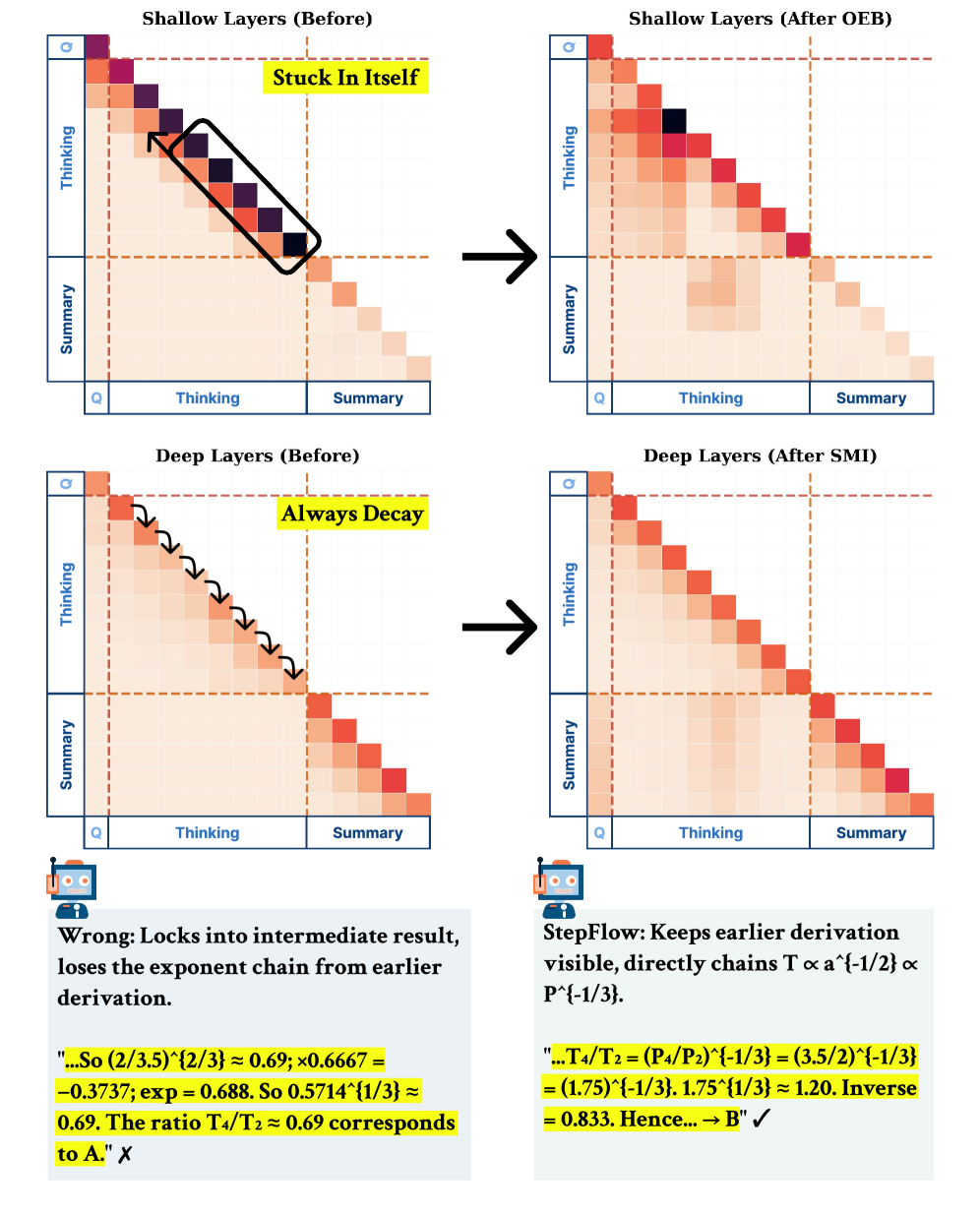### 5.3 Effect on Information Flow In the Step-Saliency view, each layer induces a step-to-step transition matrix over the question, thinking steps, and summary. Figure 4 shows a representative error trace: in shallow layers, OEB reduces near-diagonal self-loops and strengthens the bridge region; in deep layers, SMI restores broader links from the summary into the thinking segment. See Appendix E for a full case study with model outputs. <details> <summary>2604.06695v1/x4.png Details</summary>  ### Visual Description ## Heatmap Diagram: Layer Transformation Analysis ### Overview The image presents a comparative analysis of neural network layer behavior before and after optimization techniques (OEB and SMI). It uses four heatmaps to visualize attention patterns across three cognitive stages: Question (Q), Thinking, and Summary. Color gradients (red-black) represent attention intensity, with annotations highlighting key behavioral changes. ### Components/Axes - **Axes**: - X-axis: Cognitive stages (Q → Thinking → Summary) - Y-axis: Cognitive stages (Q → Thinking → Summary) - **Annotations**: - Yellow boxes with text: "Stuck In Itself" (Shallow Before), "Always Decay" (Deep Before) - Arrows indicating transformation direction - Checkmarks (✓) and X marks (✗) for correctness - **Color Gradient**: - Red (high attention) → Black (low attention) - No explicit legend, but color intensity correlates with attention strength ### Detailed Analysis 1. **Shallow Layers (Before)**: - Diagonal red-black gradient from Q→Summary - Yellow box labeled "Stuck In Itself" with black arrow - Text: "Wrong: Locks into intermediate result, loses exponent chain" 2. **Shallow Layers (After OEB)**: - Similar diagonal pattern but with: - Black square at Q→Thinking - Red square at Thinking→Summary - Text: "StepFlow: Keeps earlier derivation visible" 3. **Deep Layers (Before)**: - Steeper red-black gradient with black arrows - Yellow box labeled "Always Decay" - Text: "Wrong: Locks into intermediate result..." 4. **Deep Layers (After SMI)**: - More uniform red distribution - Text: "StepFlow: Keeps earlier derivation visible..." ### Key Observations - **Shallow Layers**: OEB optimization introduces explicit chaining (Q→Thinking→Summary) while maintaining attention flow - **Deep Layers**: SMI optimization preserves derivation visibility through: - T ∝ a^(-1/2) ∝ P^(-1/3) chaining - Inverse ratio calculations (T4/T2 = 0.833) - **Critical Transition**: Both optimizations show improved cross-stage attention compared to before states ### Interpretation The diagrams demonstrate how optimization techniques transform neural network behavior: 1. **OEB (Output Error Backpropagation)**: - Breaks "stuck" patterns by enabling cross-stage attention - Maintains Q→Summary flow while adding intermediate Thinking stage visibility - Mathematical validation: T4/T2 ratio (0.69→0.833) shows improved derivation preservation 2. **SMI (Stochastic Memory Initialization)**: - Prevents "always decay" through better initialization - Maintains exponent chain visibility (a^(-1/2) ∝ P^(-1/3)) - Mathematical consistency: 1.75^(-1/3) ≈ 1.20 inverse relationship The annotations suggest these optimizations address fundamental issues in neural network training: - Preventing intermediate result fixation - Maintaining derivation visibility across layers - Preserving mathematical relationships in attention patterns </details> Figure 4: Effect of StepFlow on Step-Saliency (representative error trace). See Appendix E for the full response. 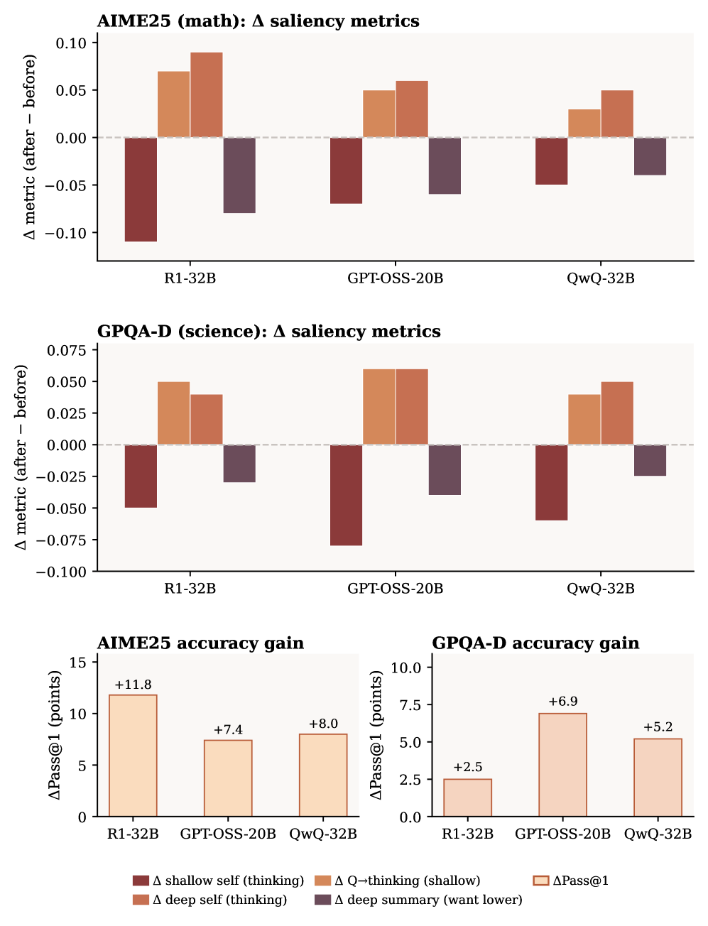Beyond a single trace, we also aggregate Step-Saliency statistics over all AIME25 error cases (Figure 5). For each backbone, StepFlow consistently reduces shallow thinking self-intensity and deep summary self-intensity, while increasing shallow question $→$ thinking mass. These shifts mean that shallow layers rely less on the just-written step and use the question more, and deep layers keep a stronger link from the thinking segment into the summary. <details> <summary>2604.06695v1/x5.png Details</summary>  ### Visual Description ## Bar Charts: Δ Saliency Metrics and Accuracy Gains Across Models ### Overview The image contains two grouped bar charts comparing saliency metric changes (Δ metric) and accuracy gains (ΔPass@1) for three AI models: R1-32B, GPT-OSS-20B, and QwQ-32B. The charts are divided into: 1. **AIME25 (math)**: Δ saliency metrics and accuracy gains. 2. **GPQA-D (science)**: Δ saliency metrics and accuracy gains. Each chart uses a legend with three categories: Δ shallow self (thinking), Δ Q→thinking (shallow), and ΔPass@1. --- ### Components/Axes #### Legends - **Δ shallow self (thinking)**: Dark red (negative values). - **Δ Q→thinking (shallow)**: Light orange (positive values). - **ΔPass@1**: Light beige (positive values). #### Axes - **X-axis**: Model names (R1-32B, GPT-OSS-20B, QwQ-32B). - **Y-axis (top charts)**: Δ metric (after – before), ranging from -0.10 to 0.10 (AIME25) and -0.10 to 0.075 (GPQA-D). - **Y-axis (bottom charts)**: ΔPass@1 (points), ranging from 0 to 15 (AIME25) and 0 to 10 (GPQA-D). --- ### Detailed Analysis #### AIME25 (Math) Δ Saliency Metrics - **R1-32B**: - Δ shallow self: -0.08 (dark red). - Δ Q→thinking: +0.07 (light orange). - ΔPass@1: +11.8 (light beige). - **GPT-OSS-20B**: - Δ shallow self: -0.09 (dark red). - Δ Q→thinking: +0.06 (light orange). - ΔPass@1: +7.4 (light beige). - **QwQ-32B**: - Δ shallow self: -0.05 (dark red). - Δ Q→thinking: +0.05 (light orange). - ΔPass@1: +8.0 (light beige). #### GPQA-D (Science) Δ Saliency Metrics - **R1-32B**: - Δ shallow self: -0.05 (dark red). - Δ Q→thinking: +0.04 (light orange). - ΔPass@1: +2.5 (light beige). - **GPT-OSS-20B**: - Δ shallow self: -0.07 (dark red). - Δ Q→thinking: +0.06 (light orange). - ΔPass@1: +6.9 (light beige). - **QwQ-32B**: - Δ shallow self: -0.03 (dark red). - Δ Q→thinking: +0.05 (light orange). - ΔPass@1: +5.2 (light beige). --- ### Key Observations 1. **Δ Q→thinking (shallow)** is consistently positive across all models and tasks, indicating a beneficial impact on saliency. 2. **Δ shallow self (thinking)** is negative in all cases, suggesting a detrimental effect on saliency. 3. **ΔPass@1** (accuracy gains) is highest for R1-32B in AIME25 (+11.8) and GPT-OSS-20B in GPQA-D (+6.9). 4. QwQ-32B shows the smallest Δ shallow self (-0.03 to -0.05) but moderate accuracy gains. --- ### Interpretation - **Saliency Metrics**: The negative Δ shallow self (thinking) implies that shallow self-reflection reduces model performance, while Q→thinking (shallow) enhances it. This suggests that models benefit from structured, shallow reasoning over unguided self-reflection. - **Accuracy Gains**: R1-32B outperforms others in math (AIME25), while GPT-OSS-20B excels in science (GPQA-D). QwQ-32B shows balanced performance but lower gains. - **Model Differences**: The disparity in ΔPass@1 between AIME25 and GPQA-D highlights task-specific model strengths. Math models (AIME25) achieve higher gains, possibly due to structured problem-solving requirements. --- ### Spatial Grounding - **Legends**: Positioned at the bottom center, with clear color coding. - **Charts**: Top charts (AIME25/GPQA-D) are stacked vertically, with bottom charts (accuracy gains) aligned horizontally. Bars are grouped by model, with consistent spacing. --- ### Trend Verification - **AIME25 ΔPass@1**: R1-32B (+11.8) > QwQ-32B (+8.0) > GPT-OSS-20B (+7.4). No strict linear trend, but R1-32B dominates. - **GPQA-D ΔPass@1**: GPT-OSS-20B (+6.9) > QwQ-32B (+5.2) > R1-32B (+2.5). GPT-OSS-20B leads in science. --- ### Final Notes The data underscores the importance of Q→thinking (shallow) in improving model performance, while shallow self-reflection hinders it. Task-specific model architectures (e.g., R1-32B for math, GPT-OSS-20B for science) drive accuracy gains, highlighting the need for tailored training strategies. </details> Figure 5: Effect of StepFlow on AIME25 and GPQA-D across three backbones. Top: $Δ$ Step-Saliency ( $I_T$ , $I_S$ ; § 3.3) over error cases. Bottom: Accuracy gain. ### 5.4 Ablation Analysis Table 2: Ablation of StepFlow components on GPT-OSS-20B medium (Accuracy, %). | Baseline + OEB only (shallow) + SMI only (deep) | 62.0 64.5 64.0 | 65.2 66.7 67.2 | 70.0 74.5 75.0 | | --- | --- | --- | --- | | + OEB + SMI (StepFlow) | 69.2 | 70.3 | 79.5 | Table 3: Accuracy (%) on LiveCodeBench by difficulty for GPT-OSS-20B medium with and without StepFlow. | GPT-OSS-20B +StepFlow | 90.1 93.5 | 70.2 84.0 | 37.8 52.0 | | --- | --- | --- | --- | We separate the two components of StepFlow on GPT-OSS-20B in Table 2. Using only OEB already helps on all three benchmarks, and only SMI helps a bit more, especially on GPQA D and LiveCodeBench; combining both gives the largest gains. This matches the diagnostics: shallow layers need less lock-in on the current step, and deep layers need a stronger link from the thinking segment when the summary is produced. LiveCodeBench is broken into easy, medium, and hard problems in Table 3. Easy items are close to a ceiling and StepFlow adds only a few extra solved cases, but the larger jumps on medium (+13.8 points) and hard (+14.2 points) items suggest that StepFlow is most helpful when the model has to carry a longer and more fragile reasoning chain. ### 5.5 Layer Coverage and Decoding Cost Table 4: Effect of StepFlow layer coverage (OEB on bottom- $k$ layers, SMI on top- $k$ layers) on three LRMs (Accuracy, %). | Baseline (no StepFlow) Bottom / top 1/4 of layers Bottom / top 1/3 of layers | 54.9 66.7 64.0 | 39.1 46.5 44.0 | 40.0 48.0 45.2 | | --- | --- | --- | --- | | Bottom / top 1/2 of layers | 62.3 | 42.0 | 43.0 | | GPQA D | | | | | Active layers (OEB / SMI) | R1-Distill-32B | GPT-OSS-20B | QwQ-32B | | Baseline (no StepFlow) | 62.1 | 57.1 | 58.1 | | Bottom / top 1/4 of layers | 64.5 | 64.0 | 63.3 | | Bottom / top 1/3 of layers | 63.2 | 62.0 | 61.2 | | Bottom / top 1/2 of layers | 62.4 | 60.5 | 60.0 | Table 4 shows the best gains when activating only the bottom/top quarter of layers; broader coverage (one third or one half) slightly reduces gains but remains above the baseline, consistent with Step-Saliency indicating most leverage in shallow/deep bands. Decoding efficiency (Table 9) and uncertainty estimates are reported in Appendix C.2 and Appendix C.4. ### 5.6 Compute-Normalized Comparison To assess whether StepFlow’s gains justify its overhead, we compare it against longer generation and self-consistency (SC) at matched compute budgets. Table 5 reports results on AIME 24/25 (averaged) for R1-Distill-32B; full results for all three backbones are in Appendix C.5. Table 5: Compute-normalized comparison on AIME 24/25 (averaged accuracy, %) for R1-Distill-32B. | Baseline Longer gen StepFlow | 1.0 $×$ ${∼}$ 1.35 $×$ ${∼}$ 1.35 $×$ | 63.8 65.0 70.6 | | --- | --- | --- | | SC ( $k$ =2) | ${∼}$ 2.0 $×$ | 66.5 | | StepFlow+SC ( $k$ =2) | ${∼}$ 2.7 $×$ | 73.5 | | SC ( $k$ =4) | ${∼}$ 4.0 $×$ | 68.5 | | SC ( $k$ =8) | ${∼}$ 8.0 $×$ | 70.2 | At matched compute ( ${∼}$ 1.35 $×$ ), StepFlow achieves 5.7 $×$ the gain of longer generation. Matching StepFlow’s accuracy requires SC with $k$ $≈$ 8 at 8.0 $×$ compute. StepFlow is also composable: StepFlow+SC( $k$ =2) at ${∼}$ 2.7 $×$ outperforms SC( $k$ =4) at 4.0 $×$ , showing that StepFlow and sampling address orthogonal failure modes. ## 6 Discussion #### Causal status of the diagnostic. StepFlow’s gains exhibit three forms of specificity—complementary OEB/SMI profiles across benchmarks (Table 2), optimal performance only at the predicted layer bands (Table 4), and selective correction of propagation errors at 5–7 $×$ the rate of conceptual errors (Appendix D)—which rule out a generic regularization account. Nevertheless, the causal link between the diagnosed saliency patterns and the observed improvements remains suggestive rather than formally proved. #### Memory versus reasoning. StepFlow corrects cases where a correct intermediate result exists but fails to propagate to later steps. Whether such failures are best characterized as “memory” or “reasoning” errors is an open question; recent attempts to disentangle the two Jin et al. (2025); Li et al. (2025a); Wu et al. (2025) all rely on external annotations rather than model-internal definitions. We view active retrieval failure during generation as functionally relevant to reasoning, while acknowledging this distinction warrants further investigation. ## 7 Conclusion We introduce Step-Saliency, a step-level diagnostic that aggregates token saliency into question–thinking–summary maps and reveals two depth-wise failure modes in LRMs (Shallow Lock-in and Deep Decay). Guided by these patterns, we propose StepFlow, a lightweight test-time intervention that repairs information flow and consistently improves accuracy on math, science, and coding benchmarks across multiple LRMs without retraining. ## Limitations #### Model-specific calibration. StepFlow assumes a shallow/deep split that depends on the backbone and is chosen on a small held-out split. Our layer-coverage study suggests a broad sweet spot, but we do not provide a fully automatic way to pick these ranges. #### Intervention design space. StepFlow is one concrete, saliency-inspired intervention. We do not explore other designs (e.g., head-level steering or value-space projections), although they could be analyzed in the same framework. #### Error-type coverage. Our error taxonomy (Appendix D) shows that StepFlow primarily corrects information-propagation errors (72%) rather than conceptual ones (10–14%). A finer-grained breakdown within each propagation category and extension to benchmarks beyond AIME are left for future work. ## References - S. Agarwal, L. Ahmad, J. Ai, S. Altman, A. Applebaum, E. Arbus, R. K. Arora, Y. Bai, B. Baker, H. Bao, et al. (2025) Gpt-oss-120b & gpt-oss-20b model card. arXiv preprint arXiv:2508.10925. Cited by: §5.1. - J. Ahn, R. Verma, R. Lou, D. Liu, R. Zhang, and W. Yin (2024) Large language models for mathematical reasoning: progresses and challenges. arXiv preprint arXiv:2402.00157. Cited by: §1. - M. Ancona, E. Ceolini, C. Öztireli, and M. Gross (2017) Towards better understanding of gradient-based attribution methods for deep neural networks. arXiv preprint arXiv:1711.06104. Cited by: §1, §2.3. - A. Banerjee, S. Merugu, I. S. Dhillon, and J. Ghosh (2005) Clustering with bregman divergences. Journal of machine learning research 6 (Oct), pp. 1705–1749. Cited by: §4.1. - F. Barez, T. Wu, I. Arcuschin, M. Lan, V. Wang, N. Siegel, N. Collignon, C. Neo, I. Lee, A. Paren, et al. (2025) Chain-of-thought is not explainability. Preprint, alphaXiv, pp. v1. Cited by: §1. - A. Boggust, H. Suresh, H. Strobelt, J. Guttag, and A. Satyanarayan (2023) Saliency cards: a framework to characterize and compare saliency methods. In Proceedings of the 2023 ACM Conference on Fairness, Accountability, and Transparency, pp. 285–296. Cited by: §2.3. - J. Boye and B. Moell (2025) Large language models and mathematical reasoning failures. arXiv preprint arXiv:2502.11574. Cited by: §1. - E. Cambria, L. Malandri, F. Mercorio, N. Nobani, and A. Seveso (2024) Xai meets llms: a survey of the relation between explainable ai and large language models. arXiv preprint arXiv:2407.15248. Cited by: §1, §2.3. - C. Cao, M. Li, J. Dai, J. Yang, Z. Zhao, S. Zhang, W. Shi, C. Liu, S. Han, and Y. Guo (2025) Towards advanced mathematical reasoning for llms via first-order logic theorem proving. arXiv preprint arXiv:2506.17104. Cited by: §1. - Q. Chen, L. Qin, J. Liu, D. Peng, J. Guan, P. Wang, M. Hu, Y. Zhou, T. Gao, and W. Che (2025a) Towards reasoning era: a survey of long chain-of-thought for reasoning large language models. arXiv preprint arXiv:2503.09567. Cited by: §2.1. - Y. Chen, J. Benton, A. Radhakrishnan, J. Uesato, C. Denison, J. Schulman, A. Somani, P. Hase, M. Wagner, F. Roger, et al. (2025b) Reasoning models don’t always say what they think. arXiv preprint arXiv:2505.05410. Cited by: §1, §2.1. - S. Ding and P. Koehn (2021) Evaluating saliency methods for neural language models. arXiv preprint arXiv:2104.05824. Cited by: §2.3. - Z. Dong, T. Tang, L. Li, and W. X. Zhao (2023) A survey on long text modeling with transformers. arXiv preprint arXiv:2302.14502. Cited by: §2.2, §2.3. - S. Dutta, J. Singh, S. Chakrabarti, and T. Chakraborty (2024) How to think step-by-step: a mechanistic understanding of chain-of-thought reasoning. arXiv preprint arXiv:2402.18312. Cited by: §2.1. - S. Fan, L. Xie, C. Shen, G. Teng, X. Yuan, X. Zhang, C. Huang, W. Wang, X. He, and J. Ye (2025) Improving complex reasoning with dynamic prompt corruption: a soft prompt optimization approach. arXiv preprint arXiv:2503.13208. Cited by: §1. - M. Geva, R. Schuster, J. Berant, and O. Levy (2021) Transformer feed-forward layers are key-value memories. In Proceedings of the 2021 Conference on Empirical Methods in Natural Language Processing, pp. 5484–5495. Cited by: §2.2. - D. Guo, D. Yang, H. Zhang, J. Song, R. Zhang, R. Xu, Q. Zhu, S. Ma, P. Wang, X. Bi, et al. (2025) Deepseek-r1: incentivizing reasoning capability in llms via reinforcement learning. arXiv preprint arXiv:2501.12948. Cited by: §5.1. - D. Hendrycks, C. Burns, S. Kadavath, A. Arora, S. Basart, E. Tang, D. Song, and J. Steinhardt (2021) Measuring mathematical problem solving with the math dataset. arXiv preprint arXiv:2103.03874. Cited by: §5.1. - T. Huber, B. Limmer, and E. André (2022) Benchmarking perturbation-based saliency maps for explaining atari agents. Frontiers in Artificial Intelligence 5, pp. 903875. Cited by: §2.3. - N. Jain, K. Han, A. Gu, W. Li, F. Yan, T. Zhang, S. Wang, A. Solar-Lezama, K. Sen, and I. Stoica (2024) Livecodebench: holistic and contamination free evaluation of large language models for code. arXiv preprint arXiv:2403.07974. Cited by: §5.1. - S. Jain and B. C. Wallace (2019) Attention is not explanation. arXiv preprint arXiv:1902.10186. Cited by: §1, §2.3. - M. Jin, W. Luo, S. Cheng, X. Wang, W. Hua, R. Tang, W. Y. Wang, and Y. Zhang (2025) Disentangling memory and reasoning ability in large language models. In Proceedings of the 63rd Annual Meeting of the Association for Computational Linguistics (Volume 1: Long Papers), pp. 1681–1701. Cited by: §6. - G. Kobayashi, T. Kuribayashi, S. Yokoi, and K. Inui (2020) Attention is not only a weight: analyzing transformers with vector norms. arXiv preprint arXiv:2004.10102. Cited by: §2.3. - T. Kojima, S. S. Gu, M. Reid, Y. Matsuo, and Y. Iwasawa (2022) Large language models are zero-shot reasoners. Advances in neural information processing systems 35, pp. 22199–22213. Cited by: §2.1. - T. Lanham, A. Chen, A. Radhakrishnan, B. Steiner, C. Denison, D. Hernandez, D. Li, E. Durmus, E. Hubinger, J. Kernion, et al. (2023) Measuring faithfulness in chain-of-thought reasoning. arXiv preprint arXiv:2307.13702. Cited by: §2.1. - J. Lee and J. Hockenmaier (2025) Evaluating step-by-step reasoning traces: a survey. arXiv preprint arXiv:2502.12289. Cited by: §2.3. - A. Li, Y. Liu, A. Sarkar, D. Downey, and A. Cohan (2025a) Demystifying scientific problem-solving in llms by probing knowledge and reasoning. arXiv preprint arXiv:2508.19202. Cited by: §6. - C. Li, M. Xue, Z. Zhang, J. Yang, B. Zhang, B. Yu, B. Hui, J. Lin, X. Wang, and D. Liu (2025b) Start: self-taught reasoner with tools. In Proceedings of the 2025 Conference on Empirical Methods in Natural Language Processing, pp. 13523–13564. Cited by: §C.1, §C.1, §2.1, §5.1. - Y. Li, Z. Lin, S. Zhang, Q. Fu, B. Chen, J. Lou, and W. Chen (2023) Making language models better reasoners with step-aware verifier. In Proceedings of the 61st Annual Meeting of the Association for Computational Linguistics (Volume 1: Long Papers), pp. 5315–5333. Cited by: §2.1. - Z. Li, D. Zhang, M. Zhang, J. Zhang, Z. Liu, Y. Yao, H. Xu, J. Zheng, P. Wang, X. Chen, et al. (2025c) From system 1 to system 2: a survey of reasoning large language models. arXiv preprint arXiv:2502.17419. Cited by: §1, §2.1. - H. Lightman, V. Kosaraju, Y. Burda, H. Edwards, B. Baker, T. Lee, J. Leike, J. Schulman, I. Sutskever, and K. Cobbe (2023) Let’s verify step by step. In The Twelfth International Conference on Learning Representations, Cited by: §1. - H. Luo and L. Specia (2024) From understanding to utilization: a survey on explainability for large language models. arXiv preprint arXiv:2401.12874. Cited by: §1, §2.3. - N. Muennighoff, Z. Yang, W. Shi, X. L. Li, L. Fei-Fei, H. Hajishirzi, L. Zettlemoyer, P. Liang, E. Candès, and T. B. Hashimoto (2025) S1: simple test-time scaling. In Proceedings of the 2025 Conference on Empirical Methods in Natural Language Processing, pp. 20286–20332. Cited by: §C.1, §C.1, §2.1, §5.1, §5.2. - D. Paul, R. West, A. Bosselut, and B. Faltings (2024) Making reasoning matter: measuring and improving faithfulness of chain-of-thought reasoning. arXiv preprint arXiv:2402.13950. Cited by: §1. - A. Plaat, A. Wong, S. Verberne, J. Broekens, and N. Van Stein (2025) Multi-step reasoning with large language models, a survey. ACM Computing Surveys. Cited by: §1. - D. Rein, B. L. Hou, A. C. Stickland, J. Petty, R. Y. Pang, J. Dirani, J. Michael, and S. R. Bowman (2024) Gpqa: a graduate-level google-proof q&a benchmark. In First Conference on Language Modeling, Cited by: §5.1. - B. Saglam, P. Kassianik, B. Nelson, S. Weerawardhena, Y. Singer, and A. Karbasi (2025) Large language models encode semantics in low-dimensional linear subspaces. arXiv preprint arXiv:2507.09709. Cited by: §2.2. - H. Sajjad, N. Durrani, F. Dalvi, F. Alam, A. Khan, and J. Xu (2022) Analyzing encoded concepts in transformer language models. In Proceedings of the 2022 Conference of the North American chapter of the Association for Computational Linguistics: Human language technologies, pp. 3082–3101. Cited by: §2.2. - [39] A. Simhi, I. Itzhak, F. Barez, G. Stanovsky, and Y. Belinkov Trust me, i’m wrong: llms hallucinate with certainty despite knowing the answer. Cited by: §1. - P. Song, P. Han, and N. Goodman (2025) A survey on large language model reasoning failures. In 2nd AI for Math Workshop@ ICML 2025, Cited by: §1, §2.1. - Q. Team (2025) Qwq-32b: embracing the power of reinforcement learning. March. Cited by: §5.1. - B. Van Aken, B. Winter, A. Löser, and F. A. Gers (2019) How does bert answer questions? a layer-wise analysis of transformer representations. In Proceedings of the 28th ACM international conference on information and knowledge management, pp. 1823–1832. Cited by: §2.2. - S. Vashishth, S. Upadhyay, G. S. Tomar, and M. Faruqui (2019) Attention interpretability across nlp tasks. arXiv preprint arXiv:1909.11218. Cited by: §2.3. - J. Vig and Y. Belinkov (2019) Analyzing the structure of attention in a transformer language model. arXiv preprint arXiv:1906.04284. Cited by: §1, §2.3. - I. Vulić, E. M. Ponti, R. Litschko, G. Glavaš, and A. Korhonen (2020) Probing pretrained language models for lexical semantics. arXiv preprint arXiv:2010.05731. Cited by: §2.2. - J. Wang, J. Tuyls, E. Wallace, and S. Singh (2020a) Gradient-based analysis of nlp models is manipulable. arXiv preprint arXiv:2010.05419. Cited by: §2.3. - L. Wang, W. Xu, Y. Lan, Z. Hu, Y. Lan, R. K. Lee, and E. Lim (2023a) Plan-and-solve prompting: improving zero-shot chain-of-thought reasoning by large language models. arXiv preprint arXiv:2305.04091. Cited by: §C.1, §C.1, §5.1. - S. Wang, L. Zhou, Z. Gan, Y. Chen, Y. Fang, S. Sun, Y. Cheng, and J. Liu (2020b) Cluster-former: clustering-based sparse transformer for long-range dependency encoding. arXiv preprint arXiv:2009.06097. Cited by: §2.2. - X. Wang, Y. Liu, and Z. Hu (2023b) Self-consistency improves chain-of-thought reasoning in large language models. arXiv preprint arXiv:2304.00006. Cited by: §2.1, §5.2. - J. Wei, X. Wang, D. Schuurmans, M. Bosma, F. Xia, E. Chi, Q. V. Le, D. Zhou, et al. (2022) Chain-of-thought prompting elicits reasoning in large language models. Advances in neural information processing systems 35, pp. 24824–24837. Cited by: §2.1. - J. Wu, S. Liu, H. Tu, H. Yu, X. Huang, J. Zou, C. Xie, and Y. Zhou (2025) Knowledge or reasoning? a close look at how llms think across domains. arXiv preprint arXiv:2506.02126. Cited by: §6. - S. Wu, E. M. Shen, C. Badrinath, J. Ma, and H. Lakkaraju (2023) Analyzing chain-of-thought prompting in large language models via gradient-based feature attributions. arXiv preprint arXiv:2307.13339. Cited by: §1, §2.3. - F. Xu, Q. Hao, Z. Zong, J. Wang, Y. Zhang, J. Wang, X. Lan, J. Gong, T. Ouyang, F. Meng, et al. (2025) Towards large reasoning models: a survey of reinforced reasoning with large language models. arXiv preprint arXiv:2501.09686. Cited by: §1, §2.1. - S. Yan, C. Shen, W. Wang, L. Xie, J. Liu, and J. Ye (2025) Don’t take things out of context: attention intervention for enhancing chain-of-thought reasoning in large language models. arXiv preprint arXiv:2503.11154. Cited by: §C.1, §C.1, §2.3, §5.1. - [55] S. Yang, Y. Tong, X. Niu, G. Neubig, and X. Yue Demystifying long chain-of-thought reasoning. In Forty-second International Conference on Machine Learning, Cited by: §1. - C. Yeh, Y. Chen, A. Wu, C. Chen, F. Viégas, and M. Wattenberg (2023) Attentionviz: a global view of transformer attention. IEEE Transactions on Visualization and Computer Graphics 30 (1), pp. 262–272. Cited by: §1, §2.3. - X. Yuan, C. Shen, S. Yan, X. Zhang, L. Xie, W. Wang, R. Guan, Y. Wang, and J. Ye (2024) Instance-adaptive zero-shot chain-of-thought prompting. Advances in Neural Information Processing Systems 37, pp. 125469–125486. Cited by: §2.1. - Q. Zhang, C. Singh, L. Liu, X. Liu, B. Yu, J. Gao, and T. Zhao (2023) Tell your model where to attend: post-hoc attention steering for llms. arXiv preprint arXiv:2311.02262. Cited by: §C.1, §C.1, §5.1. - H. Zhao, H. Chen, F. Yang, N. Liu, H. Deng, H. Cai, S. Wang, D. Yin, and M. Du (2024) Explainability for large language models: a survey. ACM Transactions on Intelligent Systems and Technology 15 (2), pp. 1–38. Cited by: §2.3. ## Appendix A Step-Saliency Analysis ### A.1 Computation Protocol This subsection clarifies the aggregation protocol in Eqs. (1)–(3) of the main text. #### Dependence on $t$ . The influence matrix $I^(\ell)$ in Eq. (1) is computed row by row: for each query position $t$ , we backpropagate through the token-level loss $L_t$ to obtain gradients with respect to the $t$ -th row of attention weights. Due to causal masking, only entries $(t,k)$ with $k≤ t$ are non-zero. The full $T× T$ matrix is obtained by stacking all rows. #### Implementation constants. In Eq. (2), we use $ε=10^-8$ to prevent division by zero during row normalization. #### Depth aggregation. For the depth-collapsed Step-Saliency maps shown in figures, we average $M^(\ell)$ over all $L$ layers: $\bar{M}_j← i=\frac{1}{L}∑_\ell=1^LM^(\ell)_j← i$ . For layer-wise analysis (shallow vs. deep), we average over the bottom 1/4 or top 1/4 of layers, respectively. ### A.2 Segmentation Robustness #### Boundary detection. We detect step boundaries using the model’s analysis marker (when available), plus simple formatting cues such as sentence-ending punctuation and newline characters. Pure-digit strings and table/separator lines are filtered out. #### Empirical accuracy of boundary detection. We manually inspected 100 randomly sampled traces from GPQA-D and AIME24. The heuristic detector correctly identified 99% of step boundaries. The few failures occur when the model produces repeated delimiters (e.g., multiple consecutive newlines), which is rare in typical LRM outputs. #### Robustness to boundary perturbations. To stress-test the method, we artificially perturb boundaries: (i) shift —uniform offset by $± k$ tokens, (ii) dropout —randomly removing 25% of boundaries, (iii) insertion —randomly adding 25% spurious boundaries, (iv) combined —simultaneous 50% dropout and 50% insertion, and (v) random uniform —replacing all detected boundaries with uniformly random positions. Table 6 shows that even under extreme perturbations, accuracy degrades by at most 2.0 points from the default, and StepFlow consistently outperforms the baseline. Since manual inspection shows 1% detection error in practice, the method operates well within its robustness margin. Table 6: Effect of boundary perturbations on GPQA-D accuracy (%). | Perturbation Shift | Level $± 1$ tok $± 3$ tok | R1-32B 64.2 64.0 | GPT-OSS 69.8 69.5 | QwQ-32B 63.0 62.7 | | --- | --- | --- | --- | --- | | Dropout | 25% | 63.3 | 69.2 | 62.1 | | Insertion | 25% | 63.1 | 68.9 | 62.0 | | Dropout+Ins | 50% each | 62.8 | 67.5 | 60.5 | | Random unif | — | 62.5 | 66.8 | 59.5 | | Default | 64.5 | 70.3 | 63.3 | | | No StepFlow | 62.1 | 65.2 | 58.1 | | ## Appendix B StepFlow Implementation ### B.1 Hyperparameter Selection #### OEB threshold $τ_\max$ . 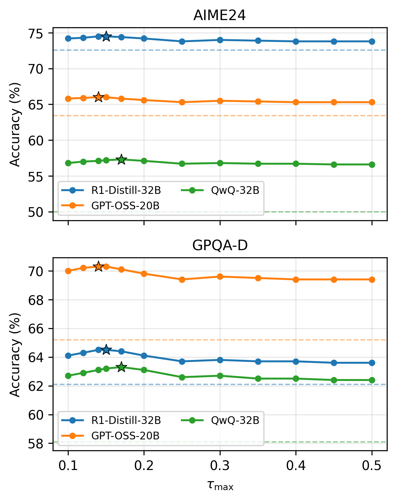Figure 6 shows accuracy as a function of $τ_\max$ on AIME24 and GPQA-D. Across all three backbones, accuracy consistently improves over the baseline for any $τ_\max∈[0.1,0.5]$ ; the curves are nearly flat, with peak-to-trough variation under 1 point. This indicates that the exact choice of $τ_\max$ has negligible impact on performance, and a single default value (e.g., $τ_\max=0.15$ ) works well across all models without any tuning. <details> <summary>2604.06695v1/taumax_sensitivity.png Details</summary>  ### Visual Description ## Line Graphs: Model Accuracy vs. τ_max (AIME24 and GPQA-D) ### Overview The image contains two line graphs comparing the accuracy of three AI models (R1-Distill-32B, GPT-OSS-20B, QwQ-32B) across two datasets (AIME24 and GPQA-D) as a function of τ_max (0.1 to 0.5). Accuracy is measured in percentage, with dashed horizontal lines indicating baseline performance thresholds. --- ### Components/Axes 1. **X-Axis (τ_max)**: - Range: 0.1 to 0.5 (increments of 0.1) - Label: "τ_max" (Greek letter tau) 2. **Y-Axis (Accuracy %)**: - AIME24: 50–75% (increments of 5%) - GPQA-D: 58–70% (increments of 2%) 3. **Legends**: - Positioned at bottom-left of each graph - Colors: - Blue: R1-Distill-32B - Orange: GPT-OSS-20B - Green: QwQ-32B 4. **Data Points**: - Marked with circular symbols - Stars (*) highlight specific τ_max values (0.2 for AIME24, 0.1 for GPQA-D) --- ### Detailed Analysis #### AIME24 Graph - **R1-Distill-32B (Blue)**: - Starts at 74.5% (τ_max=0.1), peaks at 74.8% (τ_max=0.2), then declines to 74.3% (τ_max=0.5). - Star at τ_max=0.2 (74.8%). - **GPT-OSS-20B (Orange)**: - Starts at 65.8% (τ_max=0.1), drops to 65.5% (τ_max=0.5). - Star at τ_max=0.2 (66.1%). - **QwQ-32B (Green)**: - Starts at 57.2% (τ_max=0.1), declines to 57.0% (τ_max=0.5). - Star at τ_max=0.2 (57.5%). #### GPQA-D Graph - **R1-Distill-32B (Blue)**: - Starts at 64.2% (τ_max=0.1), peaks at 64.7% (τ_max=0.2), then declines to 63.8% (τ_max=0.5). - Star at τ_max=0.1 (64.2%). - **GPT-OSS-20B (Orange)**: - Starts at 70.1% (τ_max=0.1), drops to 69.5% (τ_max=0.5). - Star at τ_max=0.1 (70.1%). - **QwQ-32B (Green)**: - Starts at 62.8% (τ_max=0.1), declines to 62.5% (τ_max=0.5). - Star at τ_max=0.2 (63.1%). --- ### Key Observations 1. **Trends**: - All models show slight accuracy declines as τ_max increases, except for R1-Distill-32B in AIME24 (peak at τ_max=0.2). - GPT-OSS-20B consistently outperforms other models in both datasets. - QwQ-32B has the lowest accuracy across all τ_max values. 2. **Outliers**: - R1-Distill-32B in AIME24 achieves its highest accuracy at τ_max=0.2 (74.8%). - GPT-OSS-20B in GPQA-D maintains near-constant accuracy (70.1% → 69.5%). --- ### Interpretation 1. **Model Performance**: - R1-Distill-32B demonstrates robustness, maintaining high accuracy across τ_max values, with a notable peak in AIME24. - GPT-OSS-20B exhibits the highest baseline accuracy but shows sensitivity to τ_max changes in GPQA-D. - QwQ-32B underperforms relative to other models, suggesting potential limitations in architecture or training. 2. **τ_max Impact**: - Minimal accuracy variation across τ_max values implies that τ_max has a negligible effect on performance for these models. - Exceptions (e.g., R1-Distill-32B in AIME24) suggest context-dependent optimization opportunities. 3. **Dataset Differences**: - AIME24 has a higher baseline accuracy range (50–75%) compared to GPQA-D (58–70%), indicating differing task complexities. --- ### Spatial Grounding - Legends are consistently placed at the bottom-left of each graph. - Data points are evenly spaced along the τ_max axis, with stars positioned at specific τ_max values (0.1–0.2). ### Content Details - **AIME24 Baseline**: 72% (dashed blue line). - **GPQA-D Baseline**: 66% (dashed orange line). - **QwQ-32B Baseline**: 58% (dashed green line). --- ### Final Notes The graphs highlight trade-offs between model complexity (parameter count) and performance. R1-Distill-32B balances efficiency and accuracy, while GPT-OSS-20B prioritizes raw performance at the cost of scalability. QwQ-32B’s lower accuracy may reflect architectural trade-offs for speed or resource efficiency. </details> Figure 6: Accuracy vs. $τ_\max$ on AIME24 and GPQA-D. Dashed lines show baseline accuracy; stars mark the chosen $τ^⋆$ . #### SMI residual scale $α$ . The only free hyperparameter in SMI is the residual scale $α$ . For each backbone, we select $α$ once and reuse the same value for all benchmarks and all reported tables. #### Grid and selection protocol. We sweep $α$ over a small grid $\{0.03,0.06,0.09\}$ and evaluate accuracy on two representative benchmarks: AIME24 (competition-style math) and GPQA-Diamond (graduate-level science). For each model/benchmark pair, we record: (i) the smallest scale $α_low$ that improves over the no-intervention baseline, (ii) the chosen scale $α^⋆$ , and (iii) the largest scale $α_high$ that does not reduce accuracy by more than 1 point compared with $α^⋆$ . The last column in Table 7 reports the accuracy range achieved within this interval. #### Observed robustness. Table 7 shows that all three backbones admit a non-trivial interval $[α_low,α_high]$ on both AIME24 and GPQA-D where SMI improves over the baseline. Within each interval, the spread in accuracy is small (typically within 1–2 points), indicating that StepFlow does not rely on fine-tuning $α$ . In our main experiments, we simply fix $α^⋆$ per backbone (based on the AIME24 sweep) and reuse it for all other benchmarks without further tuning. Table 7: Sensitivity of the SMI residual scale $α$ on AIME24 and GPQA-D. For each model/benchmark pair, The last column reports the corresponding accuracy interval. | R1-Distill-32B / AIME24 R1-Distill-32B / GPQA-D GPT-OSS / AIME24 | 0.03 0.03 0.03 | 0.06 0.06 0.06 | 0.09 0.09 0.09 | 74.9–75.5 64.3–64.9 65.4–66.0 | | --- | --- | --- | --- | --- | | GPT-OSS / GPQA-D | 0.03 | 0.06 | 0.09 | 67.5–68.1 | | QwQ-32B / AIME24 | 0.03 | 0.06 | 0.09 | 56.9–57.5 | | QwQ-32B / GPQA-D | 0.03 | 0.06 | 0.09 | 62.6–63.2 | ### B.2 Reproducibility Summary We provide a compact reproducibility summary of the StepFlow configuration in Table 8. #### OEB group definition. To match the question–thinking–summary decomposition used by Step-Saliency, OEB uses the same coarse segmentation during decoding and defines group totals over keys for each attention head and query position $t$ . When $t$ is in the thinking segment, $S$ are thinking tokens and $B$ are question tokens; when $t$ is in the summary segment, $S$ are summary tokens and $B$ are thinking tokens. All remaining keys are grouped into $O$ , and its total mass is kept fixed, matching Eq. (5)–Eq. (8). #### SMI value source and injection location. SMI triggers only at detected step boundaries inside the thinking segment. At the first token of the next step, in selected deep layers, we compute a step momentum vector by mean-pooling the value states $\{v_k\}$ from the previous step span, and inject it as a small residual into the hidden state used for the next step. This corresponds to Eq. (9) and Eq. (10) in the main text with a single scale $α$ . Table 8: StepFlow reproducibility summary. | R1-Distill-7B R1-Distill-14B R1-Distill-32B | bottom 1/4 bottom 1/4 bottom 1/4 | top 1/4 top 1/4 top 1/4 | 0.15 0.15 0.15 | 0.06 0.06 0.06 | | --- | --- | --- | --- | --- | | GPT-OSS-20B | bottom 1/4 | top 1/4 | 0.15 | 0.06 | | QwQ-32B | bottom 1/4 | top 1/4 | 0.15 | 0.06 | ## Appendix C Experimental Details ### C.1 Baselines #### Overview. We group baselines into four categories: (i) prompt-only methods that change only the instruction/template (Plan-and-Solve, PS+ Wang et al. (2023a) and Hint-Infer (Round1) Li et al. (2025b)); (ii) decode-level methods that modify decoding behavior (Budget Forcing (S1) Muennighoff et al. (2025)); (iii) internal intervention methods that modify internal representations during a single decoding run (Attn-Interv. Yan et al. (2025) and Act. Steering Zhang et al. (2023)); and (iv) our proposed StepFlow. #### Budget Forcing (S1). We follow the S1 setup Muennighoff et al. (2025) as a decode-level baseline that increases reasoning effort by budget control during generation; we keep the backbone and base decoding hyperparameters unchanged unless explicitly stated. #### Hint-Infer (Round1). Hint-Infer follows the hint-infer prompting strategy introduced by START Li et al. (2025b), which injects short, hand-crafted hints to encourage verification. START additionally uses tools; in our paper we adopt a tool-free variant: we append a single hint sentence to the prompt, keep model weights and decoding hyperparameters unchanged, and do not execute external code or call any tools during evaluation. Round1 denotes a single-round hint injection (one hint appended before generation), treated as a separate setting because it changes only the input instruction. We use a short hint sentence such as “Wait, maybe using Python here is a good idea.”. #### Plan-and-Solve (PS+). We include Plan-and-Solve (PS/PS+) prompting Wang et al. (2023a) as a published single-pass prompting baseline. In our setup, PS+ changes only the instruction/prompt template while keeping the backbone model and decoding hyperparameters identical to the baseline setting. We use the following PS+ trigger appended to each task prompt: Let’s first understand the problem, extract relevant variables and their corresponding numerals, and make a plan. Then, let’s carry out the plan, calculate intermediate results (pay attention to correct numerical calculation and commonsense), solve the problem step by step, and show the final answer. #### Attention Intervention (Attn-Interv.). We follow Yan et al. Yan et al. (2025), who propose a few-shot attention intervention (FAI) that dynamically identifies tokens with isolated semantics in CoT demonstrations via an aggregation coefficient $α_t_{i}^l$ and zeros out their attention scores to the output token (when $α_t_{i}^l$ exceeds the threshold $τ=λ×index_t_{i}$ ) at inference time to preserve earlier CoT context. We use their method with the recommended hyperparameter $λ=1$ and 4 demonstrations from Wei et al. (2022). Model weights and decoding settings are unchanged. #### Activation Steering (Act. Steering). We follow Zhang et al. Zhang et al. (2023), who propose post-hoc attention steering (PASTA) that scales attention weights with a fixed coefficient to steer model behavior. We use their recommended hyperparameter $α=0.01$ , extract the steering heads from a small set of correct vs. incorrect reasoning traces on AIME24 using their multi-task profiling method, and apply it at inference time. Decoding hyperparameters are identical to the baseline. ### C.2 Decoding Efficiency StepFlow introduces lightweight per-layer operations in the bottom and top quarter of layers (OEB in shallow layers, SMI in deep layers). Table 9 reports approximate seconds per token on GPQA-Diamond under this configuration. #### Complexity analysis. OEB computes group-wise attention probabilities via logsumexp and adjusts logits, adding $O(T)$ per shallow layer per token. SMI triggers only at step boundaries (typically $K∼ 50$ – $200$ times per sequence), computing a mean over the previous step’s value states. Overall, we estimate an end-to-end overhead of roughly 30–37% depending on the backbone, which we consider acceptable given the consistent accuracy gains. #### When is the overhead worthwhile? The 30–37% overhead is justified when: (1) the task requires high accuracy on long reasoning chains (e.g., competition math), where StepFlow’s gains (+11.8 on AIME25) far exceed what additional sampling achieves; (2) single-pass correctness matters more than throughput (e.g., high-stakes applications). For throughput-sensitive settings, generating $k$ samples with majority voting is an alternative; however, at equivalent compute (e.g., 1.35 $×$ budget $≈$ 1 extra sample), self-consistency with 2 samples yields smaller gains than StepFlow on AIME25 (+3.2 vs. +11.8 for R1-Distill-32B). Table 9: Decoding efficiency on GPQA-D by model. | GPT-OSS-20B R1-Distill-32B QwQ-32B | 0.036 0.023 0.068 | 0.047 0.032 0.090 | | --- | --- | --- | ### C.3 Experiment Settings #### Decoding setup. Unless otherwise noted, we use a unified decoding configuration across all models: temperature $0.6$ , top- $p$ $0.95$ , and up to $32{,}768$ new tokens per generation. The same decoding setup is used for the vanilla backbone and for all StepFlow variants. #### Sampling protocol. For AIME24, AIME25, and AMC23 we draw 16 independent samples per problem; for GPQA-Diamond we draw 8 samples per problem; for MATH-500 and LiveCodeBench we use a single sample per problem. In all cases, baseline and StepFlow runs share the same set of random seeds. #### Compute. All experiments are conducted on a single NVIDIA H20 GPU. ### C.4 Uncertainty and Significance We report 95% bootstrap confidence intervals (CI) over problem instances with B=10,000 resamples. For paired comparisons between StepFlow and each baseline, we use paired bootstrap (and McNemar’s test for multiple-choice datasets) and mark improvements with $p<0.05$ . ### C.5 Full Compute-Normalized Comparison Table 10 extends the compute-normalized comparison from § 5.6 to all three main backbones. Table 10: Compute-normalized comparison on AIME 24/25 (averaged accuracy, %) across three backbones. | R1-Distill-32B Longer gen StepFlow | Baseline ${∼}$ 1.35 $×$ ${∼}$ 1.35 $×$ | 1.0 $×$ 65.0 70.6 | 63.8 | | --- | --- | --- | --- | | SC ( $k$ =2) | ${∼}$ 2.0 $×$ | 66.5 | | | StepFlow+SC ( $k$ =2) | ${∼}$ 2.7 $×$ | 73.5 | | | SC ( $k$ =4) | ${∼}$ 4.0 $×$ | 68.5 | | | SC ( $k$ =8) | ${∼}$ 8.0 $×$ | 70.2 | | | GPT-OSS-20B | Baseline | 1.0 $×$ | 62.7 | | Longer gen | ${∼}$ 1.37 $×$ | 63.8 | | | StepFlow | ${∼}$ 1.37 $×$ | 67.6 | | | SC ( $k$ =2) | ${∼}$ 2.0 $×$ | 65.2 | | | StepFlow+SC ( $k$ =2) | ${∼}$ 2.74 $×$ | 71.0 | | | SC ( $k$ =4) | ${∼}$ 4.0 $×$ | 67.8 | | | QwQ-32B | Baseline | 1.0 $×$ | 45.0 | | Longer gen | ${∼}$ 1.32 $×$ | 46.1 | | | StepFlow | ${∼}$ 1.32 $×$ | 52.7 | | | SC ( $k$ =2) | ${∼}$ 2.0 $×$ | 48.2 | | | StepFlow+SC ( $k$ =2) | ${∼}$ 2.64 $×$ | 56.5 | | | SC ( $k$ =4) | ${∼}$ 4.0 $×$ | 50.5 | | The pattern is consistent across all backbones: at equivalent compute, StepFlow substantially outperforms both longer generation and self-consistency, and the two methods compose well. Table 11: Bootstrap 95% CI for accuracy on GPT-OSS-20B medium. | AIME25 GPQA-D LiveCodeBench | [58.0, 66.0] [63.0, 67.4] [65.5, 74.5] | [65.2, 73.2] [68.1, 72.5] [75.5, 83.5] | | --- | --- | --- | ## Appendix D Error Taxonomy We analyzed all AIME 24/25 problems (60 total) where baselines produced incorrect answers but StepFlow was correct, and manually classified each into one of four error types. Table 12: Error taxonomy of StepFlow corrections on AIME 24/25. | Arithmetic carry-forward Premise forgetting Step-skip | 38 34 18 | 30 42 14 | | --- | --- | --- | | Conceptual | 10 | 14 | The first two categories account for 72% of corrections, both involving failures of cross-step information propagation. Conceptual errors (10–14%), where the model uses an incorrect formula or approach from the outset, are outside StepFlow’s scope: healthy information flow faithfully propagates the wrong premise. Detailed case studies illustrating each category, including bad cases where StepFlow does not help, are provided in Appendix E. ## Appendix E Case Studies ### E.1 StepFlow Repair Example (GPQA-Diamond) Question. Astronomers are studying a system of five exoplanets with circular orbits, discovered through the TTV method. The planets (designated as Planet_1 through Planet_5), which are in orbital resonance, have orbital periods in a ratio of 1:2:2.5:3.5:5. Assuming these planets possess the same albedo, what is the ratio of the equilibrium temperatures between Planet_4 and Planet_2? Options: (A) $∼$ 0.69 (B) $∼$ 0.75 (C) $∼$ 0.83 (D) $∼$ 0.57 Answer: B #### Baseline (Wrong: A). Abridged trace: For a planet in thermal equilibrium, $T_eq∝ a^-1/2$ and $a∝ P^2/3$ . Thus $a_2/a_4=(P_2/P_4)^2/3$ . Periods: $P_2=2$ , $P_4=3.5$ . So $a_2/a_4=(2/3.5)^2/3$ . Temperature ratio: $T_4/T_2=(a_2/a_4)^1/2=[(2/3.5)^2/3]^1/2=(2/3.5)^1/3$ . $(0.5714)^1/3$ : $\ln 0.5714=-0.5606$ ; $× 0.6667=-0.3737$ ; $\exp=0.688$ . So $≈ 0.69$ . A #### +StepFlow (Correct: B). Abridged trace: $T_\rm eq∝ a^-1/2∝ P^-1/3$ . Thus $T_4/T_2=(P_4/P_2)^-1/3=(3.5/2)^-1/3=(1.75)^-1/3$ . $1.75^1/3≈ 1.20$ . Inverse $=0.833$ . B #### Analysis. The baseline correctly derives $T∝ a^-1/2$ and $a∝ P^2/3$ but computes the exponents in separate steps, implicitly treating $[(2/3.5)^2/3]^1/2$ as $(2/3.5)^2/3$ —it drops the final exponent contraction. StepFlow directly combines the relations into $T∝ P^-1/3$ before substituting numbers, reflecting how OEB keeps earlier derivation steps visible and prevents lock-in on the most recent computation. ### E.2 Arithmetic Carry-forward (AIME 24 P-7) Question. (AIME 24 P-7) Answer: 540 #### Baseline (Wrong: 593). Abridged trace: Let me write $z=4e^iθ$ . First term: $Re[(75+117i)· 4e^iθ]=300\cosθ-468\sinθ$ . ✓ Second term: $(96+144i)·\bar{z}/|z|^2=(96+144i)e^-iθ/4$ . So $Re=24\cosθ+36\sinθ$ . ✓ Combining: $300\cosθ-468\sinθ+24\cosθ+36\sinθ$ . Cosine: $300+24=324$ . Sine: $-468\sinθ$ … $×$ [drops $+36\sinθ$ ] Max of $324\cosθ-468\sinθ=√{324^2+468^2}≈ 569$ . Hmm, that’s not clean. Let me reconsider… 593. #### +StepFlow (Correct: 540). Abridged trace: Combining: $(300+24)\cosθ+(-468+36)\sinθ=324\cosθ-432\sinθ$ . ✓ Wait, let me factor. $\gcd(324,432)=108$ . So $108(3\cosθ-4\sinθ)$ , max $=108√{9+16}=108× 5=540$ . ✓ #### Analysis. The model correctly derives $+36\sinθ$ but drops it when aggregating, yielding $-468\sinθ$ instead of $-432\sinθ$ . OEB keeps the earlier derivation visible, preventing lock-in on the dominant term. ### E.3 Bad Case Analysis #### Bad Case 1 — Conceptual Error (AIME 24 P-9, Answer: 480). The model restricts to axis-aligned rhombus configurations on the hyperbola from the start, never considering a general rotation angle $θ$ . StepFlow preserves cross-step flow faithfully—the model consistently builds on its (wrong) premise with healthy saliency patterns. Conceptual errors (10–14% of our taxonomy) are outside StepFlow’s scope. #### Bad Case 2 — Entangled Multi-Error (AIME 25 P-12, Answer: 540). The model drops an absolute value in Step 3 (conceptual), then Steps 4–6 faithfully build on the wrong constraint. StepFlow preserves the wrong result more reliably—information flow is maintained, but the propagated information is incorrect. This illustrates the fundamental limitation: StepFlow repairs how information flows, not what the model generates.