2604.06699v1

# Adaptive Prompt Structure Factorization: A Framework for Self-Discovering and Optimizing Compositional Prompt Programs ## Abstract Automated prompt optimization is crucial for eliciting reliable reasoning from large language models (LLMs), yet most API-only prompt optimizers iteratively edit monolithic prompts, coupling components and obscuring credit assignment, limiting controllability, and wasting tokens. We propose Adaptive Prompt Structure Factorization (aPSF), an API-only framework (prompt-in/text-out; no access to model internals) that uses an Architect model to discover task-specific prompt structures as semantic factors. aPSF then performs interventional, single-factor updates: interventional factor-level scoring estimates each factor’s marginal contribution via validation-performance changes, and error-guided factor selection routes updates to the current dominant failure source for more sample-efficient optimization. Across multiple advanced reasoning benchmarks, aPSF outperforms strong baselines including principle-aware optimizers, improving accuracy by up to +2.16 percentage points on average, and reduces optimization cost by 45–87% tokens on MultiArith while reaching peak validation in 1 step. Adaptive Prompt Structure Factorization: A Framework for Self-Discovering and Optimizing Compositional Prompt Programs Haoyue Liu $\spadesuit$ Zhichao Wang $\spadesuit$ Yongxin Guo $\heartsuit$ Haoran Shou $\spadesuit$ Xiaoying Tang $\spadesuit$ * $\spadesuit$ The Chinese University of Hong Kong, Shenzhen $\heartsuit$ Taobao and Tmall Group {haoyueliu, zhichaowang, haoranshou}@link.cuhk.edu.cn guoyongxin.gyx@taobao.com tangxiaoying@cuhk.edu.cn footnotetext: Corresponding author. footnotetext: Code available at https://github.com/luckyboyLiu/aPSF ## 1 Introduction <details> <summary>2604.06699v1/Fig/MOTIVATION-new.png Details</summary>  ### Visual Description ## Diagram: Comparative Analysis of Prompt Optimization Methods (OPRO vs. aPSF) ### Overview The diagram compares two prompt optimization methodologies: **Monolithic Prompting Optimization (OPRO)** and **Adaptive Prompt Structure Factorization (aPSF)**. Both workflows involve iterative refinement of prompts to improve LLM output quality, but differ in architectural design and feedback mechanisms. ### Components/Axes #### Monolithic Prompting Optimization (OPRO) 1. **Core Components**: - **Question**: Input query (top-left, human icon) - **Initial Prompt**: Starting template (green document icon) - **LLM**: Language Model (blue gear icon) - **Answer**: Generated response (pencil icon) - **Evaluator**: Quality assessment module (blue circle with checkmark) - **Prompt Optimizer**: Refinement engine (red atom icon) - **Best Prompt**: Final optimized prompt (green document icon) 2. **Flow**: - Question → Initial Prompt → LLM → Answer - Answer → Evaluator (✓/✗ feedback) - ❌ Answer → Prompt Optimizer → LLM (iterative loop) - ✓ Answer → Best Prompt (termination) 3. **Visual Elements**: - Red X for incorrect answers - Green checkmark for correct answers - Thumbs-up icon for successful evaluation #### Adaptive Prompt Structure Factorization (aPSF) 1. **Core Components**: - **Architect LLM**: Decomposition module (purple gear icon) - **Worker LLM**: Execution module (blue gear icon) - **Factors**: - Directive (snowflake icon) - Format (fire icon) - Rationale (snowflake icon) - **Error Signal**: Feedback loop (red arrow) 2. **Flow**: - Question → Initial Prompt → Architect LLM - Architect LLM → Factors → Worker LLM → Answer - Answer → Error Signal (↔️ loop to Architect LLM) - ✓ Answer → Best Prompt (termination) 3. **Visual Elements**: - Dashed box for factor decomposition - Red arrow for error signal feedback - Thumbs-up icon for successful evaluation ### Detailed Analysis #### OPRO Workflow 1. **Initialization**: Starts with a question and initial prompt 2. **Generation**: LLM produces an answer 3. **Evaluation**: Binary feedback (✓/✗) determines next steps 4. **Optimization**: Incorrect answers trigger prompt refinement 5. **Termination**: Correct answers produce the "Best Prompt" #### aPSF Workflow 1. **Decomposition**: Architect LLM breaks prompts into modular factors 2. **Parallel Processing**: Factors are processed independently 3. **Error Handling**: Explicit feedback loop for incorrect answers 4. **Modular Optimization**: Each factor can be refined separately 5. **Structured Output**: Final prompt maintains factor integrity ### Key Observations 1. **Feedback Mechanisms**: - OPRO uses binary evaluation (correct/incorrect) - aPSF implements continuous error signaling 2. **Architectural Complexity**: - OPRO: Linear workflow with single LLM - aPSF: Hierarchical architecture with specialized components 3. **Optimization Scope**: - OPRO: Global prompt refinement - aPSF: Component-wise optimization ### Interpretation The diagram reveals fundamental differences in optimization philosophy: - **OPRO** represents traditional iterative refinement, suitable for simple QA tasks where binary feedback suffices - **aPSF** introduces structural decomposition, enabling: - Parallel processing of prompt components - Targeted error correction - More nuanced feedback through error signals - The error signal loop in aPSF suggests superior adaptability to complex tasks requiring multi-faceted responses - OPRO's simplicity may offer faster convergence for straightforward problems The visual representation emphasizes that aPSF's modular approach could potentially handle more complex reasoning tasks through its factor-based architecture, while OPRO's monolithic design prioritizes simplicity and direct feedback. 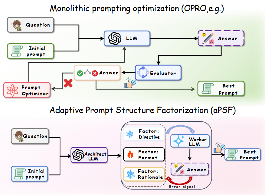</details> Figure 1: Monolithic prompt optimization vs. aPSF. Top: monolithic API-only prompt optimizers iteratively edit a single prompt. Bottom: aPSF decomposes the prompt into semantic factors and updates selected factors while freezing the rest. Large language models (LLMs) exhibit strong capabilities in reasoning, coding, and complex generation (Achiam et al., 2023; Wei et al., 2022; Kojima et al., 2022; Wang et al., 2022; Brown et al., 2020), yet their performance is highly sensitive to prompt design (Zhao et al., 2021; Liu et al., 2023). Under API-only (query-only) access, prompt optimizers typically improve performance by iteratively editing a prompt and selecting candidates by validation score (Zhou et al., 2022; Yang et al., 2023; Pryzant et al., 2023; Fernando et al., 2023; Guo et al., 2023; Deng et al., 2022; Tang et al., 2025). Early approaches such as APE (Zhou et al., 2022) and OPRO (Yang et al., 2023) treat the prompt as a holistic, indivisible string, proposing and selecting entirely new prompts at each iteration. Figure 1 contrasts monolithic prompt editing with aPSF’s factor-wise optimization. However, prompt-level edits to a monolithic prompt have three limitations. First, coupled edits obscure which prompt component caused an improvement, complicating credit assignment. Second, monolithic prompts offer weak controllability, preventing selective freezing of constraint-critical parts such as output schemas. Third, because a single mutation often perturbs multiple functional roles at once, many trials are confounded and rejected for unrelated reasons, wasting query budget and slowing convergence. In practice, effective prompts often behave like compositional programs with semantic factors (e.g., task interpretation, reasoning procedure, output format, verification) (White, 2023). Edit-based optimizers such as ProTeGi (Pryzant et al., 2023) and GrIPS (Prasad et al., 2023) partially address this by applying localized mutations. However, without an explicit, persistent factorization, their optimization and selection still operate at the level of the full prompt, leaving credit assignment implicit and limiting selective freezing. These limitations motivate our central question: Can we automatically induce a task-specific prompt factorization and optimize factors independently, enabling explicit credit assignment and adaptive allocation of the query budget? 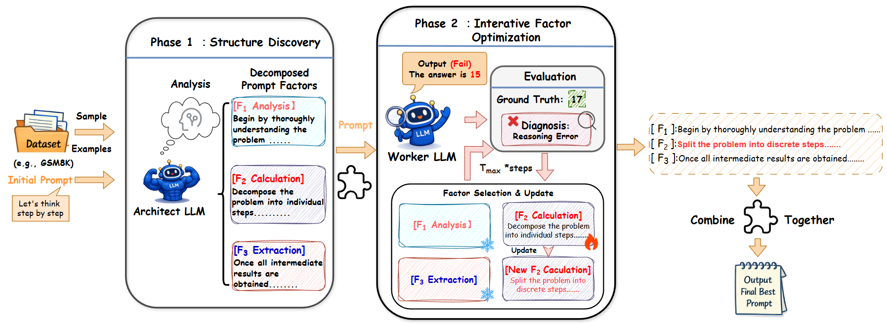To bridge this gap, we introduce Adaptive Prompt Structure Factorization (aPSF), a two-phase framework for API-only prompt optimization that incorporates: (1) adaptive structure discovery, where an Architect LLM induces a task-specific factor schema and initializes factor contents (optionally conditioned on a user-provided initial prompt); and (2) interventional factor optimization, where we edit one factor at a time and use error-guided factor selection to route updates to the current bottleneck factor. Contributions. Building on this framework, our contributions are fourfold. (1) We first decompose prompts into task-specific semantic factors, enabling precise, surgical single-factor edits while freezing the remaining factors. Under strictly API-only access, this factorization enables factor-level meta-attribution, effectively opening the black box of prompt engineering. (2) We propose interventional factor-level scoring to quantify the marginal contribution of each component, transforming prompt optimization into a traceable diagnostic process that directly maps refinement decisions to observed validation failures. (3) We develop an error-guided factor selection strategy that adaptively routes the black-box query budget to identified bottleneck factors, thereby maximizing sample efficiency and optimization stability. (4) Across six reasoning benchmarks, aPSF consistently outperforms strong baselines and yields more stable and interpretable optimization trajectories. ## 2 Related Work API-only prompt optimization. Gradient-based methods such as AutoPrompt (Shin et al., 2020), Prompt Tuning (Lester et al., 2021), and Prefix-Tuning (Li and Liang, 2021) require white-box access and thus are unsuitable for API-based models. API-only optimizers therefore rely on prompt-level search and editing, e.g., APE (Zhou et al., 2022), OPRO (Yang et al., 2023), ProTeGi (Pryzant et al., 2023), and GrIPS (Prasad et al., 2023). While candidate generation can be holistic or localized, these methods typically operate on a monolithic prompt and select candidates at the whole-prompt level, leaving component-level credit assignment implicit and limiting controllability. Recent principle-aware methods such as CriSPO (He et al., 2025) and ZERA (Yi et al., 2025) improve upon monolithic editing by generating structured critiques or evolving principles to guide prompt refinement. However, these principles serve as evaluation criteria for feedback generation rather than an explicit edit space: the optimization still proposes and selects whole-prompt candidates, limiting factor-level attribution and selective freezing. To address these limitations without changing the API-only setting, aPSF introduces an explicit factorized representation and optimizes via interventional, single-factor substitutions, making improvements attributable and controllable, even under tight query budgets. Programmatic prompting and modular pipelines. Frameworks such as DSPy (Khattab et al., 2024) and SAMMO (Schnabel and Neville, 2024) optimize prompts and demonstrations within a user-specified program scaffold, while modularization/faceting work studies decomposition under predefined taxonomies or rules (Yao et al., 2023; Juneja et al., 2025). These approaches improve prompts within a designer-provided scaffold, but optimization and selection remain end-to-end at the program level, yielding limited component-wise attribution under query-only feedback. In contrast, aPSF automatically induces the scaffold as semantic factors and optimizes via single-factor interventions with explicit attribution, enabling selective freezing (e.g., output format). Related optimization techniques. Bandit-style allocation (Auer et al., 2002) and self-refinement methods (Madaan et al., 2023; Shinn et al., 2023; Chen et al., 2024) motivate adaptive routing and iterative improvement. However, most prior approaches treat the prompt/output as the unit of action, making it difficult to localize which component should be revised under query-only signals. aPSF instead routes updates over prompt factors via error-guided selection and applies interventional single-factor edits. ## 3 Adaptive Prompt Structure Factorization We now detail aPSF’s factorized prompt representation and optimization procedure (Figure 2); pseudocode for Phase 2 is provided in Algorithm 1 (Appendix A). <details> <summary>2604.06699v1/Fig/new-overview-new.png Details</summary>  ### Visual Description ## Flowchart: Two-Phase Prompt Optimization Process ### Overview The flowchart illustrates a two-phase process for optimizing prompts using large language models (LLMs). Phase 1 focuses on **Structure Discovery** to decompose problems into analytical components, while Phase 2 employs **Iterative Factor Optimization** to refine prompts through error correction and factor updates. The process concludes with a combined "Final Best Prompt" output. --- ### Components/Axes #### Phase 1: Structure Discovery - **Inputs**: - Dataset (e.g., GSM8K examples) - Initial Prompt: "Let's think step by step" - **Core Component**: - **Architect LLM** (blue robot icon) - Outputs: Decomposed Prompt Factors - **[F1 Analysis]**: "Begin by thoroughly understanding the problem" - **[F2 Calculation]**: "Decompose the problem into individual steps" - **[F3 Extraction]**: "Once all intermediate results are obtained" - **Flow**: Dataset → Initial Prompt → Architect LLM → Decomposed Factors #### Phase 2: Iterative Factor Optimization - **Inputs**: - Worker LLM (blue robot with magnifying glass) - Output (Fail): "The answer is 15" (incorrect) - **Evaluation**: - Ground Truth: 17 - Diagnosis: "Reasoning Error" - **Factor Selection & Update**: - Retained Factors: - **[F1 Analysis]** - **[F3 Extraction]** - Updated Factor: - **[F2 Calculation]** → **[New F2 Calculation]**: "Split the problem into discrete steps" - **Flow**: Worker LLM → Evaluation → Factor Update → Combine → Final Prompt --- ### Detailed Analysis #### Phase 1: Structure Discovery 1. **Dataset**: Contains problem examples (e.g., GSM8K). 2. **Initial Prompt**: Generic instruction to "think step by step." 3. **Architect LLM**: Analyzes the problem and decomposes it into three factors: - **F1 Analysis**: Problem comprehension. - **F2 Calculation**: Stepwise decomposition. - **F3 Extraction**: Aggregation of intermediate results. #### Phase 2: Iterative Factor Optimization 1. **Worker LLM**: Executes the initial prompt but produces an incorrect output (15 vs. ground truth 17). 2. **Evaluation**: Identifies a "Reasoning Error" in the Worker LLM's output. 3. **Factor Update**: - **F2 Calculation** is revised to emphasize "discrete steps" instead of "individual steps." - Other factors (F1, F3) remain unchanged. 4. **Combination**: Updated factors are merged into the **Final Best Prompt**. --- ### Key Observations 1. **Iterative Refinement**: Phase 2 introduces a feedback loop to correct errors by updating specific factors. 2. **Factor Prioritization**: Only F2 Calculation is modified, suggesting it was the primary source of error. 3. **Modular Design**: Factors are treated as discrete, updatable components, enabling targeted improvements. --- ### Interpretation This process demonstrates a systematic approach to prompt engineering: - **Phase 1** establishes a foundational structure by breaking down problems into analyzable components. - **Phase 2** uses error diagnosis to iteratively refine the most critical factor (F2), improving the LLM's ability to handle complex reasoning tasks. - The final prompt integrates updated factors, likely enhancing accuracy by addressing stepwise decomposition flaws. The process mirrors scientific method principles: hypothesis (initial prompt), testing (Worker LLM output), error analysis, and hypothesis revision (factor updates). </details> Figure 2: Overview of aPSF. Given a dataset of sampled examples and an optional initial prompt, aPSF proceeds in two phases. (1) Structure Discovery: the Architect LLM analyzes the task and decomposes the prompt into $K$ semantic factors $\{F_k\}_k=1^K$ (task-specific factorization, rather than a fixed scaffold). (2) Iterative Factor Optimization: the Worker LLM executes the composed prompt; an evaluator returns scores and representative failure cases, which are summarized into an error diagnosis (e.g., reasoning error: 15 vs 17). Conditioned on the diagnosis, the architect model selects a bottleneck factor for a single-factor update while freezing the remaining factors, yielding attributable, interventional prompt edits and returning the best-performing prompt within $T_\max$ steps. ### 3.1 Problem Setup and Notation Let $D_val$ and $D_test$ denote the validation and test sets, where each example is a pair $(q,y)$ of query $q$ and ground-truth answer $y$ . We denote by $p$ a prompt, by $M_W(q;p)$ the Worker LLM’s output on $q$ under $p$ , and by $s(·,·)$ a task-specific scoring function. We denote by $T$ the task description and by $X$ optional exemplars. Standard objective. Most API-only prompt optimizers cast prompt search as maximizing a validation score. We define the empirical score of prompt $p$ on dataset $D$ as $$ \hat{S}(p,D)\triangleq\frac{1}{|D|}∑_(q,y)∈Ds(M_W(q;p),y). \tag{1} $$ We optimize prompts on $D_val$ via query-only evaluation and report results on the held-out $D_test$ : $$ p^⋆=\operatorname*{arg max}_p \hat{S}(p,D_val). \tag{2} $$ Traditional monolithic optimization and limitations. Existing API-only prompt optimizers typically treat $p$ as a single string and apply global edits (Zhou et al., 2022; Yang et al., 2023; Pryzant et al., 2023; Prasad et al., 2023). At step $t$ , $Edit(p^(t);T,X)$ proposes candidates $C^(t)$ and updates $p^(t{+1)}=\operatorname*{arg max}_c∈C^(t)\hat{S}(c,D_val)$ . This design has two limitations: (1) global edits couple semantic components, obscuring credit assignment; (2) coupling prevents selectively freezing components (e.g., output format) and induces a large, unstructured search space. Addressing the limitations via factorization. To address the above limitations, we represent a prompt $p$ as an ordered list of $K$ (task-adaptive) semantic factors. Let $G=(F_1,…,F_K)$ denote the ordered factor schema, where each $F_k$ specifies one factor role, and let $B=(f_1,…,f_K)$ be the corresponding factor texts. We assemble $p$ by concatenation in schema order: $$ p=Assemble(B)\triangleqconcat(f_1,f_2,…,f_K), \tag{3} $$ where $concat(·)$ joins the text blocks with newline delimiters. Inducing task-specific factors. Instead of committing to a fixed taxonomy, we use an Architect LLM $M_A$ to induce task-specific semantic factors from $(T,X)$ . In principle, factorized prompt optimization jointly chooses schema $G$ and contents $B$ : $$ G^*,B^*=\operatorname*{arg max}_G,B\hat{S}(Assemble(B),D_val). \tag{4} $$ This joint search is intractable; we instead obtain an initialization $(G,B^(0))$ via one-pass meta-prompted generation from $M_A$ (Appendix C). ### 3.2 Phase 1: Adaptive Structure Discovery In Phase 1, the Architect LLM induces an ordered factor schema $G$ and initializes the factor contents $B^(0)$ . We support two operational modes for structure discovery: From-scratch mode. Given task description $T$ and optional exemplars $X$ , the Architect LLM $M_A$ autonomously proposes a factor schema $G$ (defining roles and sequence) and initial content $B^(0)$ : $$ \displaystyleG \displaystyle=M_A(p_struct^meta;T,X), \displaystyle B^(0) \displaystyle=M_A(p_factorinit^meta;G,T,X). \tag{5} $$ We denote by $p_struct^meta$ and $p_factorinit^meta$ the meta-prompts for schema induction and factor initialization (Appendix C). Initial-prompt mode. Let $p_init$ denote an initial prompt provided by the user (e.g., “Let’s think step by step”). aPSF analyzes its core reasoning approach and generates a task-specific extension. The Architect receives: $$ G,B^(0)=M_A(p_analyze^meta;p_init,T,X), \tag{0} $$ where $p_analyze^meta$ instructs the architect to: (1) understand the core reasoning approach of $p_init$ , (2) generate a complete task-specific instruction embodying and extending this approach, and (3) decompose it into independently optimizable factors. The meta-prompt additionally encourages preserving the initial prompt’s reasoning style while producing a fluent, compact factorization (Appendix C). ### 3.3 Phase 2: Interventional Factor Optimization #### 3.3.1 Interventional Single-Factor Updates Interventional factor-wise updates. aPSF performs coordinate-style updates by performing a single-factor edit while freezing the others, and evaluates candidates via controlled substitutions. Formally, let $B^(t)$ denote the factor contents at iteration $t$ , and $p^(t)=Assemble(B^(t))$ be the current prompt. To optimize factor $F_k$ , the Architect LLM $M_A$ proposes $N$ candidate edits $C_k^(t)=\{c_k^(j)\}_j=1^N$ . We isolate each candidate’s context-conditioned marginal contribution via contrastive evaluation. Let $B^(t)[k← c]$ replace factor $k$ by $c$ : $$ \displaystyle p^(t)_k← c \displaystyle=Assemble(B^(t)[k← c]), \displaystyleScore(c) \displaystyle=\hat{S}(p^(t)_k← c,D_val), \tag{8} $$ where all other factors are held fixed. Let $Δ\hat{S}(c)=Score(c)-\hat{S}(p^(t),D_val)$ denote the validation-score gain of candidate $c$ , and select the best candidate edit $\hat{c}_k=\operatorname*{arg max}_c∈C_k^(t)Δ\hat{S}(c)$ . We accept the update if $Δ\hat{S}(\hat{c}_k)≥δ$ and run for at most $T_\max$ steps, returning the best-performing prompt on $D_val$ . The complete procedure is detailed in Algorithm 1 (Appendix A). #### 3.3.2 Error-Guided Factor Selection After a warm-start pass that optimizes each factor once, at each step $t$ we evaluate the current prompt on $D_val$ and collect representative failure cases. We then summarize errors into a lightweight error profile and provide it to the Architect $M_A$ to select the bottleneck factor for the next update (e.g., Rationale for reasoning failures, Format for formatting errors). Concretely, we use $M_A$ with a fixed, task-agnostic meta-prompt to produce open-ended diagnoses for each failure (Appendix C.4); for reporting we summarize the diagnoses into a lightweight error profile, while factor selection conditions on representative samples and the full diagnosis. This error-guided routing makes the optimization adaptive: the update budget is dynamically reallocated to whichever factor is most responsible for current failures. If the same factor is repeatedly selected without improvement, $M_A$ may explore alternative factors to avoid local optima. We stop early once $\hat{S}(p^(t),D_val)=1$ ; Figure 15 (Appendix) provides an execution trace. | Methods | Qwen2.5-7B-Instruct (Worker) | Llama-3.1-8B-Instruct (Worker) | | | | | | | | | | --- | --- | --- | --- | --- | --- | --- | --- | --- | --- | --- | | GSM8K | AQUA | Multi | Hard | Avg | GSM8K | AQUA | Multi | Hard | Avg | | | Zero-shot CoT | 86.22 $±$ 0.00 | 81.50 $±$ 0.00 | 96.46 $±$ 0.00 | 53.79 $±$ 0.00 | 79.49 | 82.81 $±$ 0.00 | 68.00 $±$ 0.00 | 95.21 $±$ 0.00 | 33.60 $±$ 0.00 | 69.91 | | Architect = Qwen3-8B | | | | | | | | | | | | OPRO | 87.63 $±$ 1.85 | 77.00 $±$ 3.42 | 98.75 $±$ 0.38 | 53.60 $±$ 2.91 | 79.25 | 84.95 $±$ 1.67 | 64.50 $±$ 4.23 | 96.46 $±$ 0.52 | 33.62 $±$ 3.58 | 69.88 | | APE | 88.83 $±$ 0.92 | 81.50 $±$ 2.76 | 98.54 $±$ 0.61 | 51.70 $±$ 3.84 | 80.14 | 83.48 $±$ 2.13 | 66.00 $±$ 3.15 | 96.67 $±$ 0.73 | 33.05 $±$ 4.12 | 69.80 | | ProTeGi | 88.43 $±$ 1.53 | 79.50 $±$ 3.89 | 98.54 $±$ 0.44 | 53.88 $±$ 2.36 | 80.09 | 81.07 $±$ 2.78 | 62.50 $±$ 4.51 | 96.46 $±$ 0.68 | 33.52 $±$ 3.27 | 68.39 | | GrIPS | 88.16 $±$ 2.14 | 80.50 $±$ 2.93 | 98.54 $±$ 0.57 | 52.56 $±$ 3.45 | 79.94 | 83.55 $±$ 1.89 | 69.00 $±$ 3.67 | 96.67 $±$ 0.49 | 32.86 $±$ 4.38 | 70.52 | | ZERA | 89.98 $±$ 0.63 | 81.36 $±$ 0.75 | 98.42 $±$ 0.43 | 53.22 $±$ 0.94 | 80.75 | 84.15 $±$ 0.80 | 65.95 $±$ 0.95 | 98.22 $±$ 0.38 | 34.58 $±$ 0.89 | 70.73 | | CriSPO | 89.40 $±$ 0.69 | 81.48 $±$ 0.97 | 98.94 $±$ 0.58 | 55.94 $±$ 0.98 | 81.44 | 89.49 $±$ 0.83 | 65.86 $±$ 0.68 | 96.49 $±$ 0.65 | 34.94 $±$ 0.51 | 71.70 | | aPSF | 90.03 $±$ 0.71 | 82.50 $±$ 1.83 | 99.30 $±$ 0.32 | 54.77 $±$ 1.94 | 81.65 +0.21 | 85.62 $±$ 0.85 | 71.50 $±$ 2.36 | 98.33 $±$ 0.41 | 35.98 $±$ 2.47 | 72.86 +1.16 | | Architect = gpt-oss-120b | | | | | | | | | | | | OPRO | 88.70 $±$ 1.42 | 78.50 $±$ 3.68 | 97.29 $±$ 0.83 | 51.69 $±$ 3.21 | 79.05 | 85.25 $±$ 1.56 | 67.50 $±$ 3.94 | 95.21 $±$ 0.91 | 34.47 $±$ 3.82 | 70.61 | | APE | 87.36 $±$ 2.31 | 80.00 $±$ 2.84 | 86.46 $±$ 2.15 | 54.55 $±$ 2.67 | 77.09 | 80.20 $±$ 2.45 | 64.00 $±$ 4.27 | 96.88 $±$ 0.64 | 31.07 $±$ 4.53 | 68.04 | | ProTeGi | 89.70 $±$ 1.18 | 80.50 $±$ 3.25 | 98.12 $±$ 0.56 | 55.59 $±$ 2.83 | 80.98 | 84.48 $±$ 1.73 | 53.00 $±$ 4.86 | 97.50 $±$ 0.52 | 35.88 $±$ 3.14 | 67.72 | | GrIPS | 90.80 $±$ 1.76 | 82.00 $±$ 2.51 | 98.54 $±$ 0.48 | 53.41 $±$ 3.57 | 81.19 | 84.28 $±$ 2.08 | 68.00 $±$ 3.42 | 96.88 $±$ 0.71 | 32.95 $±$ 3.96 | 70.53 | | ZERA | 89.55 $±$ 0.60 | 80.31 $±$ 0.75 | 99.59 $±$ 0.89 | 52.63 $±$ 0.85 | 80.52 | 89.69 $±$ 0.21 | 68.43 $±$ 0.51 | 98.15 $±$ 0.78 | 34.70 $±$ 0.84 | 72.74 | | CriSPO | 90.11 $±$ 0.73 | 80.99 $±$ 0.65 | 99.35 $±$ 0.51 | 51.25 $±$ 0.53 | 80.43 | 90.13 $±$ 0.89 | 65.13 $±$ 0.84 | 97.90 $±$ 1.10 | 35.16 $±$ 1.15 | 72.08 | | aPSF | 90.87 $±$ 0.63 | 83.00 $±$ 1.52 | 99.53 $±$ 0.29 | 55.86 $±$ 1.68 | 82.32 +1.13 | 86.22 $±$ 0.78 | 72.50 $±$ 2.18 | 97.92 $±$ 0.36 | 42.96 $±$ 2.31 | 74.90 +2.16 | Table 1: Test accuracy (%) on math reasoning benchmarks (mean ${}_±std$ over 5 runs; ). Multi = MultiArith; Hard = GSM-Hard. All methods start from the same seed prompt (“Let’s think step by step”). Bold = best; underline = second best. Light blue rows highlight aPSF with gains in green. ## 4 Experiments Experimental questions. In this section, we conduct experiments to address the following questions: - Q1: Can aPSF achieve competitive performance compared to strong API-only prompt optimizers under identical experimental conditions? See Section 4.2. - Q2: Does aPSF provide interpretable optimization behavior and component-level insights? See Section 4.3.1 and Section 4.3. - Q3: Does aPSF improve optimization efficiency, measured by total optimization tokens and steps to reach peak validation accuracy? See Section 4.4. - Q4: Can aPSF generalize across tasks and transfer prompts across related datasets? See Section 4.5. ### 4.1 Experimental Setup and Protocol Benchmarks and baselines. We evaluate on GSM8K (Cobbe et al., 2021), AQUA-RAT (Ling et al., 2017), MultiArith (Roy and Roth, 2015), GSM-Hard (Gao et al., 2022), BBH (Srivastava et al., 2023; Suzgun et al., 2023) (17 representative sub-tasks), and MMLU (Hendrycks et al., 2020). We compare against state-of-the-art API-only prompt optimizers: OPRO (Yang et al., 2023), ProTeGi (Pryzant et al., 2023), APE (Zhou et al., 2022), GrIPS (Prasad et al., 2023), ZERA (Yi et al., 2025), CriSPO (He et al., 2025), and the unoptimized initial prompt baseline (Zero-shot CoT, i.e., using $p_init$ without optimization). All methods share the same Worker model, optimization budget, and fixed 50-example validation slice, and start from the same initial prompt $p_init$ ; for aPSF, the initial factorization step is included in $T_\max$ . We report final metrics on held-out test sets. Additional results on Competition Mathematics (Hendrycks et al., 2021) and GPQA (Rein et al., 2024) are in Appendix G. <details> <summary>2604.06699v1/Fig/bbh_subtasks_algorithm_final.png Details</summary>  ### Visual Description ## Bar Chart: BBH Sub-tasks Performance Comparison ### Overview The chart compares the accuracy of six AI models across 18 sub-tasks in the BBH (Big Bench Hard) benchmark. Models include zero-shot cot, ProTeGi, OPRO, GRIPS, APE, and aPSF. Accuracy values range from 0 to 1, with higher values indicating better performance. ### Components/Axes - **X-axis (Tasks)**: 18 sub-tasks, including "boolean expressions," "causal judgement," "date understanding," "formal fallacies," "geometric shapes," "hyperbaton," "logical deduction five objects," "logical deduction seven objects," "logical deduction three objects," "movie recommendation," "multistep arithmetic two," "object counting," "reasoning about colored objects," "ruin names," "arithmetic shuffled five objects," "tracking shuffled seven objects," and "tracking shuffled three objects". - **Y-axis (Accuracy)**: Scale from 0 to 1, with increments of 0.1. - **Legend**: Located in the top-right corner, mapping colors to models: - Orange: zero-shot cot - Blue: ProTeGi - Green: OPRO - Yellow: GRIPS - Cyan: APE - Red: aPSF ### Detailed Analysis - **Task Groups**: Each task has six grouped bars, one per model. Bars are ordered according to the legend (left to right: orange, blue, green, yellow, cyan, red). - **Accuracy Values**: Labeled on top of each bar. For example: - "boolean expressions": aPSF (0.97), ProTeGi (0.95), GRIPS (0.94), OPRO (0.93), APE (0.94), zero-shot cot (0.92). - "geometric shapes": aPSF (0.56), ProTeGi (0.42), OPRO (0.42), GRIPS (0.42), APE (0.42), zero-shot cot (0.42). - "logical deduction three objects": aPSF (0.89), ProTeGi (0.94), GRIPS (0.92), OPRO (0.85), APE (0.88), zero-shot cot (0.87). ### Key Observations 1. **aPSF Dominance**: Consistently achieves the highest accuracy across most tasks (e.g., 0.97 in "boolean expressions," 0.96 in "logical deduction seven objects"). 2. **Zero-shot cot Lag**: Generally underperforms other models (e.g., 0.42 in "geometric shapes," 0.54 in "logical deduction seven objects"). 3. **Model-Specific Strengths**: - ProTeGi excels in "logical deduction three objects" (0.94) and "tracking shuffled three objects" (0.86). - OPRO performs well in "reasoning about colored objects" (0.82) and "arithmetic shuffled five objects" (0.69). - GRIPS shows strength in "object counting" (0.70) and "tracking shuffled seven objects" (0.68). 4. **Low-Performance Tasks**: "Geometric shapes" and "ruin names" are challenging for most models, with accuracies below 0.6. ### Interpretation The data highlights **aPSF** as the most robust model, achieving near-perfect accuracy in foundational tasks like "boolean expressions" and maintaining high performance in complex reasoning tasks. In contrast, **zero-shot cot** struggles across nearly all tasks, suggesting limitations in zero-shot learning without additional context. Models like **ProTeGi** and **OPRO** demonstrate competitive performance in specific sub-tasks, indicating specialized strengths. The disparity in accuracy between models underscores the importance of architectural design and training strategies for handling diverse reasoning challenges. Outliers like "geometric shapes" (lowest accuracy: 0.42 for zero-shot cot) and "logical deduction three objects" (highest accuracy: 0.94 for ProTeGi) reveal task-specific bottlenecks and opportunities for improvement. 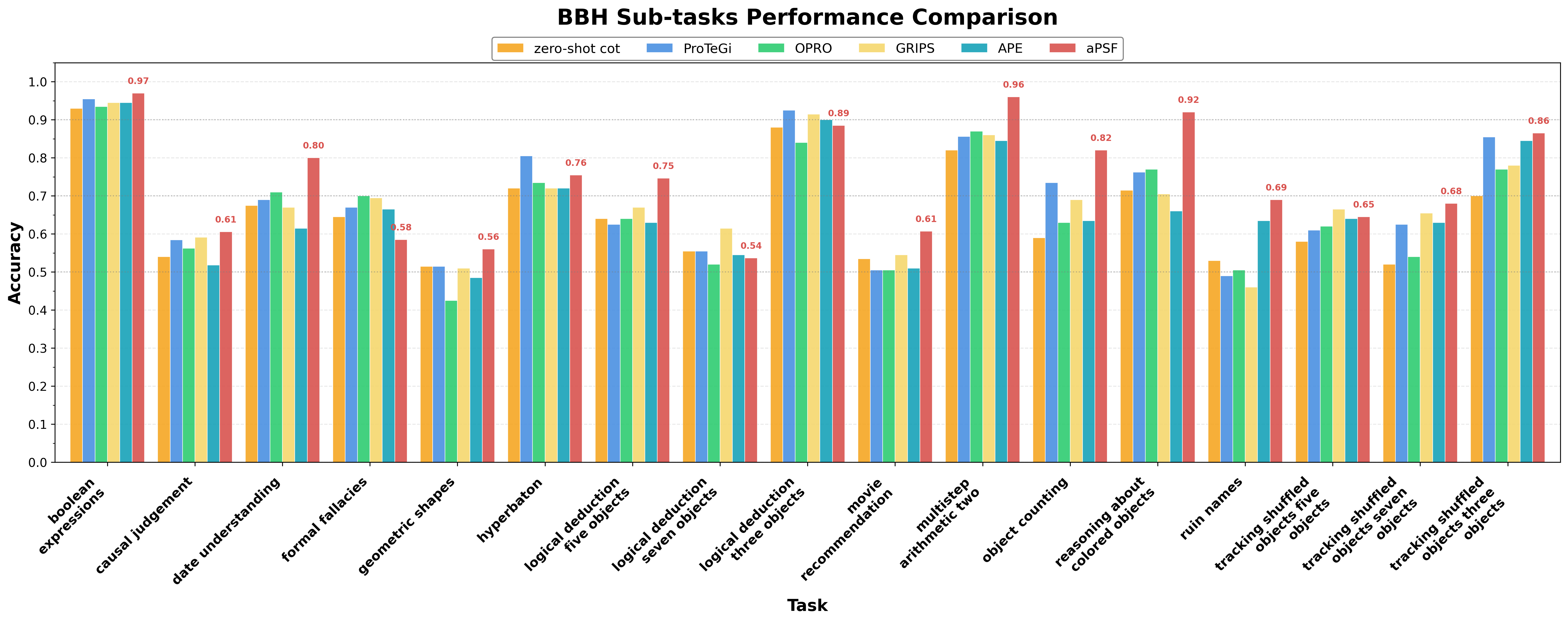</details> Figure 3: Per-task accuracy on BBH benchmarks. aPSF (red) achieves dominant performance on arithmetic and symbolic reasoning tasks, such as Multistep Arithmetic (0.96) and Boolean Expressions (0.97). Models and hyperparameters. We use Qwen2.5-7B-Instruct (Team et al., 2024) as the default Worker LLM and Qwen3-8B (Yang et al., 2025) as the Architect LLM. We additionally evaluate with Llama-3.1-8B-Instruct (Dubey et al., 2024) as Worker and gpt-oss-120b (OpenAI, 2025) as Architect to test generalization. Architect quality can affect optimization; we report results with multiple Architects (Table 1). Throughout, we restrict ourselves to query-only access (prompt in, text out), without using model internals (e.g., gradients or logits). We run the Worker with temperature=0 for deterministic scoring and set the Architect temperature to 0.7 to encourage diverse candidate generation. Unless otherwise specified, we use $N{=}4$ candidates per update (Appendix H), an acceptance threshold $δ{=}1/|D_val|$ (requiring at least one additional correct validation example), and cap optimization at $T_\max{=}10$ steps. We also instruct the Architect to prefer concise factorizations to avoid over-fragmentation. The factorization is induced by the Architect per task (Section 3.2). Due to stochasticity in candidate generation, we run the full optimization pipeline 5 times and report average test accuracy; all methods use the same protocol. Complete configurations are provided in Appendix N. ### 4.2 Q1: aPSF Achieves the Best Accuracy Under Matched Budgets We evaluate aPSF under matched API-only settings on (i) mathematical reasoning benchmarks (Table 1), (ii) diverse BBH reasoning sub-tasks (Figure 3), and (iii) a budget-matched comparison to programmatic prompting (DSPy; Table 2). Additional results on MMLU are reported in Appendix F. As shown in Table 1, Figure 3, and Table 2, we observe that: | Method | GSM8K | AQUA | GSM-Hard | MATH | | --- | --- | --- | --- | --- | | DSPy | 89.83 | 81.00 | 51.59 | 52.80 | | aPSF | 90.03 | 82.50 | 54.77 | 56.00 | | $Δ$ | +0.20 | +1.50 | +3.18 | +3.20 | Table 2: Comparison with DSPy under matched settings. MATH = Competition Mathematics (Hendrycks et al., 2021). 1. Matched-performance: aPSF achieves the best Avg in all Worker/Architect settings on different benchmarks (Table 1), improving over the strongest baseline (including principle-aware methods CriSPO and ZERA) by up to +2.16 pp and reaching 74.90% (vs 72.74%) in the strongest setting. 1. Broad coverage: on BBH, aPSF shows consistent improvements across diverse reasoning patterns, with particularly strong margins on long-context, state-tracking tasks. 1. Programmatic baselines: under a controlled, budget-matched setup, aPSF outperforms DSPy across all datasets reported, suggesting advantages from task-adaptive factorization and error-guided updates beyond fixed program scaffolds. #### 4.2.1 Q1-BBH: Complex Reasoning We evaluate aPSF on 17 representative BBH sub-tasks covering arithmetic, symbolic, logical, and temporal reasoning. Figure 3 reports per-task accuracies against baselines. aPSF delivers the largest gains on Multistep Arithmetic Two (+9.0pp vs OPRO) and Reasoning about Colored Objects (+15.0pp), consistent with improved long-context state tracking from factorizing the prompt into separable components (e.g., step-wise reasoning and consistency checks). Beyond these extremes, aPSF achieves high absolute accuracy on symbolic and state-tracking tasks such as Boolean Expressions (0.97), Web of Lies (0.905), and Tracking Shuffled Objects Three (0.86). It also improves logical deduction (e.g., +4.5pp on Logical Deduction Three Objects). This robustness is further reflected in the performance profile: within 10% of the best method ( $τ{=}0.1$ ), aPSF succeeds on 76% of BBH tasks vs. 65% for OPRO (Figure 12). #### 4.2.2 Q1-DSPy: Comparison to Programmatic Prompting <details> <summary>2604.06699v1/Fig/FIG2_final_optimized_wide.png Details</summary>  ### Visual Description ## Heatmap and Bar Chart: Factor Selection Analysis in aPSF Framework with Initial CoT Prompts ### Overview The image contains two visualizations: 1. **Heatmap (A)**: Shows factor selection rates across datasets and categories. 2. **Bar Chart (B)**: Displays test accuracy by dominant factor for each dataset. --- ### Components/Axes #### Heatmap (A) - **Title**: "Factor Selection Heatmap Across Datasets and Categories" - **X-Axis (Factor Categories)**: - Problem Analysis - Step Breakdown - Mathematical Operations - Calculation Execution - Scientific Principle - Domain Specific - **Y-Axis (Datasets)**: - GPQA Chemistry - GSM-Hard - MULTIARITH - AQUA-RAT - GSM8K - BBH Date - BBH Logic-5 - GPQA Physics - **Color Scale**: Blue (0%) to Red (100%) for selection rates. - **Legend**: Located on the right, labeled "Selection Rate (%)". #### Bar Chart (B) - **Title**: "Test Accuracy by Dominant Factor" - **X-Axis (Datasets)**: - GPQA Chemistry - GSM-Hard - MULTIARITH - AQUA-RAT - GSM8K - BBH Date - BBH Logic-5 - GPQA Physics - **Y-Axis (Test Accuracy)**: Percentage (%) from 0% to 100%. - **Legend**: - Math Tasks (Blue) - Science Tasks (Red) - Logic Tasks (Green) - **Bar Colors**: Match legend labels (e.g., blue for Math Tasks). --- ### Detailed Analysis #### Heatmap (A) - **Key Values**: - **GPQA Chemistry**: Problem Analysis (40%), Calculation Execution (50%), Scientific Principle (10%). - **GSM-Hard**: Problem Analysis (67%), Mathematical Operations (33%). - **MULTIARITH**: Problem Analysis (100%). - **AQUA-RAT**: Calculation Execution (50%), Domain Specific (30%). - **GSM8K**: Problem Analysis (30%), Calculation Execution (50%). - **BBH Date**: Domain Specific (100%). - **BBH Logic-5**: Step Breakdown (80%). - **GPQA Physics**: Scientific Principle (70%), Calculation Execution (20%). #### Bar Chart (B) - **Test Accuracy by Dataset**: - **GPQA Chemistry**: Science Tasks (30.2%). - **GSM-Hard**: Math Tasks (53.8%). - **MULTIARITH**: Math Tasks (99.3%). - **AQUA-RAT**: Calculation Execution (82.0%). - **GSM8K**: Calculation Execution (90.0%). - **BBH Date**: Domain Specific (75.3%). - **BBH Logic-5**: Step Breakdown (74.7%). - **GPQA Physics**: Scientific Principle (36.2%). --- ### Key Observations 1. **Heatmap Trends**: - Problem Analysis and Calculation Execution are frequently selected across datasets (e.g., 100% in MULTIARITH, 50% in AQUA-RAT). - Domain Specific and Step Breakdown show lower selection rates (e.g., 0% in GSM-Hard, 80% in BBH Logic-5). 2. **Bar Chart Trends**: - Math Tasks dominate in MULTIARITH (99.3%) and GSM-Hard (53.8%). - Calculation Execution is critical for GSM8K (90.0%) and AQUA-RAT (82.0%). - Science Tasks and Logic Tasks have lower accuracy in GPQA Chemistry (30.2%) and BBH Logic-5 (74.7%), respectively. --- ### Interpretation - **Factor Selection vs. Accuracy**: - Datasets with high selection rates for specific factors (e.g., MULTIARITH’s 100% Problem Analysis) correlate with high test accuracy in related tasks (Math Tasks: 99.3%). - Domain-specific factors (e.g., BBH Date’s 100% Domain Specific) show moderate accuracy (75.3%), suggesting less generalization. - **Anomalies**: - GSM-Hard has high Problem Analysis selection (67%) but lower Math Task accuracy (53.8%) compared to MULTIARITH. - GPQA Physics has high Scientific Principle selection (70%) but only 36.2% accuracy, indicating potential misalignment between factor selection and task performance. - **Implications**: - Problem Analysis and Calculation Execution are critical for Math Tasks, while Domain Specific factors are less impactful. - Science and Logic Tasks require targeted factor selection (e.g., Step Breakdown for BBH Logic-5). --- ### Spatial Grounding - **Heatmap**: Left side, with color intensity indicating selection rates. - **Bar Chart**: Right side, with bars aligned to datasets and colored by task type. - **Legends**: Heatmap’s color scale on the right; bar chart’s legend at the top right. --- ### Final Notes - All textual elements (labels, axis titles, legends) are transcribed. - Percentages are approximate, with explicit uncertainty noted (e.g., "~30%"). - No non-English text is present. 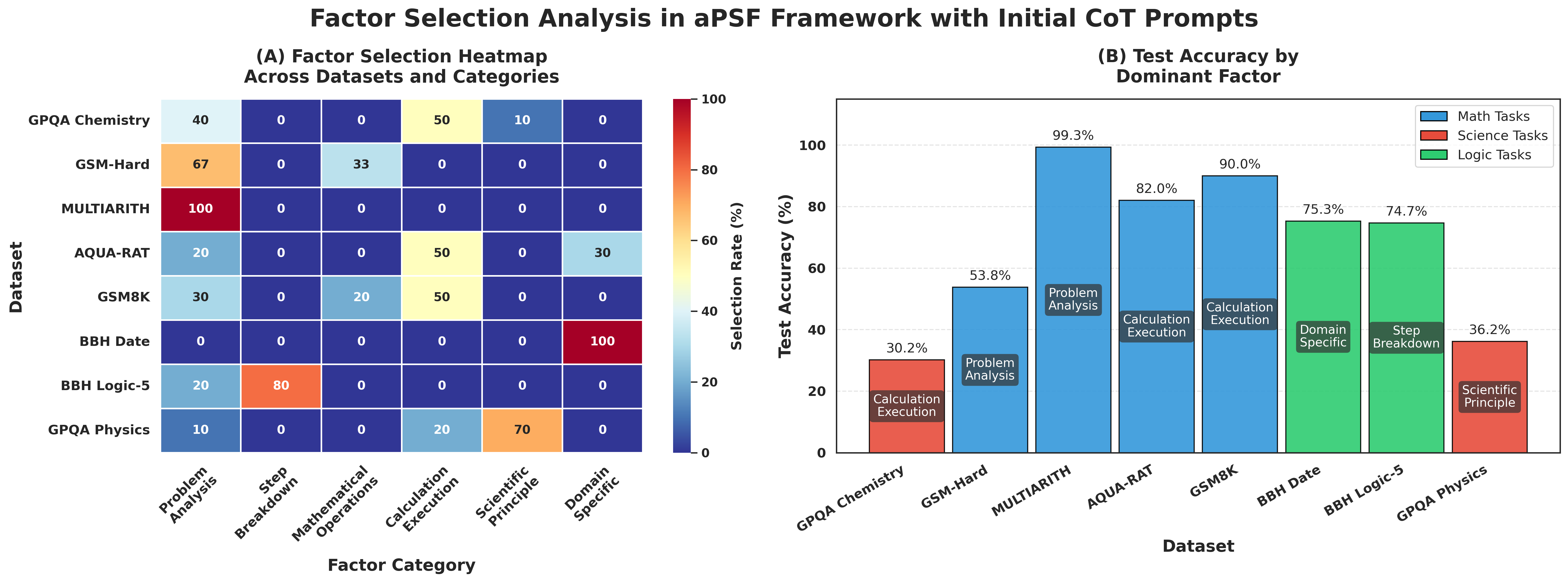</details> Figure 4: Factor selection patterns and performance. (A) Selection rate heatmap grouped by semantic category (original names in Appendix K). (B) Test accuracy and dominant factors per task (color indicates domain). We compare aPSF with DSPy (Khattab et al., 2024), a programmatic prompting framework that compiles prompts and demonstrations for a fixed, user-specified program scaffold. For a budget-matched setup, we use a single ChainOfThought module and compile it with BootstrapFewShotWithRandomSearch, running 10 trials ( $T_\max{=}10$ ) on the same validation slice, without finetuning or external data. Both methods use the same Worker (Qwen2.5-7B-Instruct) and the same compiler/optimizer LLM (Qwen3-8B) for prompt proposal/compilation. As shown in Table 2, aPSF outperforms DSPy on all reported datasets, which we attribute to task-adaptive factorization and error-guided updates rather than DSPy’s fixed single-module scaffold. Programmatic systems (e.g., SAMMO) and task-faceting methods (Juneja et al., 2025) are discussed in Related Work but are not evaluated, as their interfaces and scaffold assumptions conflict with our query-only setting. | Task | aPSF | NoStructure | Gain ( $↑$ ) | | --- | --- | --- | --- | | GSM8K | 90.03 | 89.55 | +0.48 | | AQUA-RAT | 82.50 | 79.50 | +3.00 | | Date Understanding | 80.00 | 74.00 | +6.00 | | Web of Lies | 90.50 | 85.30 | +5.20 | | Movie Recommendation | 60.72 | 58.67 | +2.05 | | Average | 80.75 | 77.40 | +3.35 | Table 3: System-level ablation. Task-specific factorization is critical for logical reasoning tasks (e.g., Date Understanding), yielding significant gains (+6.00pp) over fixed templates. ### 4.3 Q2: Routing Is Interpretable and Structure Matters We analyze optimization behavior via routing patterns across tasks and controlled ablations of structure, scheduling, and factor freezing (Figure 4, Table 3, Figure 6, Table 4, Table 6). As shown, we observe that: 1. Interpretable routing: error-guided factor selection yields task-adaptive factor usage aligned with domain needs (e.g., math emphasizes Problem Analysis / Calculation Execution; science emphasizes Scientific Principle), and the dominant factors correlate with strong per-task accuracy (Figure 4). 1. Structure matters: removing task-specific factorization (NoStructure) causes a sizable average drop (3.35pp) and disproportionately hurts format-sensitive BBH tasks, indicating generic templates miss critical procedural structure (Table 3). | Method | GSM8K | AQUA | Average | | --- | --- | --- | --- | | Error-Guided | $90.03$ | $82.50$ | $86.27$ +1.53 | | Thompson | $90.57$ | $78.00$ | $84.29$ | | Round-robin | $90.03$ | $79.00$ | $84.52$ | | Greedy | $89.97$ | $79.50$ | $84.74$ | | Random | $89.80$ | $79.50$ | $84.65$ | Table 4: Scheduler ablation on GSM8K and AQUA (Accuracy %). Error-Guided achieves the best average, while Thompson sampling shows higher variance across datasets. 1. Actionable components: factor-level knock-outs identify which components are bottlenecks (Figure 6), and scheduler ablations show error-guided factor selection improves stability and average accuracy versus alternative update strategies (Table 4). 1. Single-factor updates: unfrozen multi-factor edits degrade accuracy by an average of 1.03pp, confirming that freezing non-target factors improves credit assignment and optimization stability (Table 6). #### 4.3.1 Q2-Routing: Adaptive Patterns Across Tasks We analyze how error-guided factor selection allocates optimization effort across tasks (Figure 4). Task-adaptive optimization. Figure 4 shows task-specific routing patterns: math concentrates on Problem Analysis / Calculation Execution, logic relies on Step Breakdown or Domain Specific factors, and science emphasizes Scientific Principle. Dominant factors align with stronger test accuracy, indicating domain-specific factor priorities. Discovered schemas and trajectories are in Appendix K (Tables 13 and 14) and Appendix S (Figures 14 and 15). #### 4.3.2 Q2-Ablations: Component Knock-Outs We analyze component importance via system-level structure and factor-level sensitivity. | Source | Target Dataset | | | | | | --- | --- | --- | --- | --- | --- | | GSM8K | AQUA | MultiArith | GSM-Hard | MATH | | | MultiArith | 89.76 | 81.50 | – | 52.98 | 52.80 | | GSM8K | – | 82.00 | 99.30 | 54.08 | 51.60 | | GSM-Hard | 89.27 | 80.50 | 99.30 | – | 51.00 | | AQUA | 90.31 | – | 99.30 | 53.78 | 52.20 | | Same-task | 90.03 | 82.50 | 99.30 | 54.77 | 56.00 | Table 5: Cross-task transfer results. Prompts optimized on source tasks, evaluated on targets. Last row: same-task baseline. MATH = Competition Mathematics (Hendrycks et al., 2021). System-level: Impact of Structure. We compare against NoStructure, a fixed template without task-specific factorization. As shown in Table 3, accuracy drops by 3.35pp on average: the effect is small on GSM8K ( $-0.48$ pp) but larger on format-sensitive BBH tasks (e.g., Date Understanding: 80.0 $→$ 74.0, $-6.0$ pp), indicating generic templates miss procedural structure. Factor-level: Fine-grained Sensitivity. 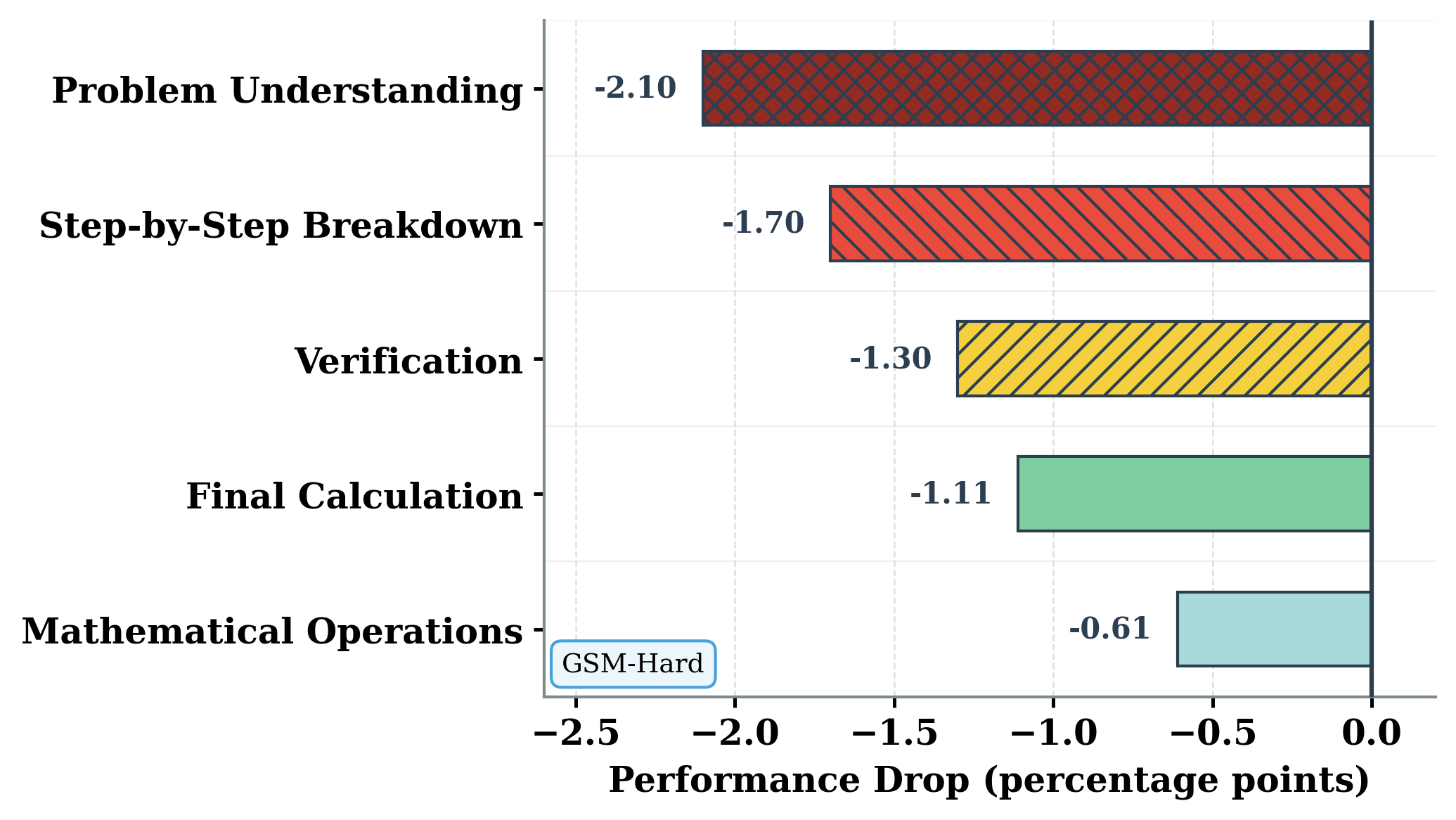Fig. 6 masks individual factors on GSM-Hard. Removing Problem Understanding causes the largest drop ( $-2.10$ pp), while Mathematical Operations has a smaller effect ( $-0.61$ pp), suggesting the Worker handles much of the arithmetic internally. #### 4.3.3 Q2-Scheduler: Ablations We compare error-guided factor selection with Round-robin, Thompson Sampling, and Greedy under identical settings (Table 4). Error-Guided achieves the best average across GSM8K and AQUA (86.27%), while Thompson sampling attains the highest GSM8K score but degrades on AQUA, indicating higher variance. This supports the claim that adaptive factor selection based on step-level error analysis improves stability without sacrificing overall quality. #### 4.3.4 Q2-Freezing: Single-Factor vs. Multi-Factor Updates To validate the single-factor update mechanism, we compare aPSF’s default frozen single-factor updates against an unfrozen variant that allows edits to modify multiple factors per step. Under the same budget ( $T_\max{=}10$ ), Worker/Architect setup, and evaluation protocol, the unfrozen variant consistently underperforms (Table 6). | Dataset | Frozen | Unfrozen | Gain ( $↑$ ) | | --- | --- | --- | --- | | AQUA-RAT | 82.50 | 81.50 | +1.00 | | MultiArith | 99.30 | 97.08 | +2.22 | | GSM-Hard | 54.77 | 54.36 | +0.41 | | Date Understanding | 80.00 | 79.50 | +0.50 | | Average | 79.14 | 78.11 | +1.03 | Table 6: Frozen (single-factor) vs. unfrozen (multi-factor) updates. Freezing non-target factors yields higher accuracy by preventing credit-assignment noise from coupled edits. When factors are unfrozen, edits spill over to adjacent factors, confounding credit assignment and producing noisier trajectories. This confirms that single-factor interventions improve stability and attribution, corroborating the coordinate-descent design in Section 3.3.1. 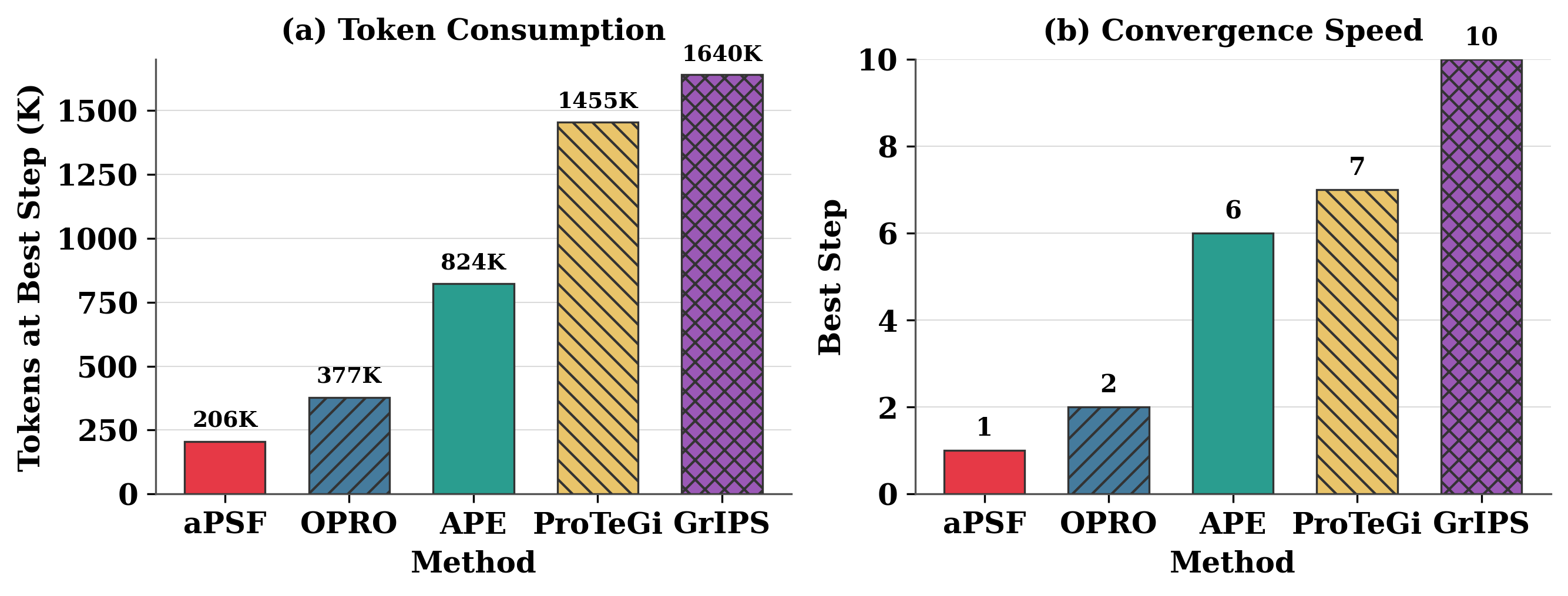### 4.4 Q3: aPSF Reaches Peak Validation in 1 Step with 45–87% Fewer Tokens We analyze efficiency on MultiArith (Figure 5) along two axes: total optimization tokens and steps-to-best (the number of optimization iterations until the run attains its maximum validation accuracy). Total optimization tokens include both Architect generation (structure discovery and candidate proposals) and Worker evaluation (validation inference) across all steps. As shown in Figure 5, we observe that: 1. Token efficiency: aPSF reaches peak validation accuracy with 206K tokens (45–87% fewer than baselines). 1. Convergence speed: aPSF reaches peak validation accuracy at step 1 (vs. 6–10 steps for others). 1. Generalization: This efficiency advantage generalizes across datasets; on GSM8K, AQUA, and GSM-Hard, aPSF consistently reaches peak validation earlier with 36–55% fewer tokens than OPRO and ZERA (Appendix R.5). <details> <summary>2604.06699v1/Fig/token_efficiency_combined.png Details</summary>  ### Visual Description ## Bar Charts: Token Consumption and Convergence Speed by Method ### Overview The image contains two side-by-side bar charts comparing five computational methods (aPSF, OPRO, APE, ProTeGi, GrIPS) across two metrics: **Token Consumption** (measured in thousands of tokens, K) and **Convergence Speed** (measured in "Best Step" units). Both charts use color-coded bars with distinct patterns for visual differentiation. --- ### Components/Axes #### Chart (a): Token Consumption - **X-axis**: Methods (aPSF, OPRO, APE, ProTeGi, GrIPS) - **Y-axis**: Tokens at Best Step (K), scaled from 0 to 1500 in increments of 250 - **Legend**: - Red (solid): aPSF - Blue (diagonal stripes): OPRO - Teal (solid): APE - Yellow (diagonal stripes): ProTeGi - Purple (crosshatch): GrIPS #### Chart (b): Convergence Speed - **X-axis**: Same methods as Chart (a) - **Y-axis**: Best Step, scaled from 0 to 10 in increments of 2 - **Legend**: Same color patterns as Chart (a) --- ### Detailed Analysis #### Chart (a): Token Consumption - **aPSF**: 206K tokens (red bar, shortest) - **OPRO**: 377K tokens (blue bar, second shortest) - **APE**: 824K tokens (teal bar, mid-range) - **ProTeGi**: 1455K tokens (yellow bar, second tallest) - **GrIPS**: 1640K tokens (purple bar, tallest) #### Chart (b): Convergence Speed - **aPSF**: 1 step (red bar, shortest) - **OPRO**: 2 steps (blue bar, second shortest) - **APE**: 6 steps (teal bar, mid-range) - **ProTeGi**: 7 steps (yellow bar, second tallest) - **GrIPS**: 10 steps (purple bar, tallest) --- ### Key Observations 1. **Token Consumption Trends**: - Token usage increases monotonically from aPSF (206K) to GrIPS (1640K). - ProTeGi and GrIPS consume significantly more tokens than other methods. 2. **Convergence Speed Trends**: - Convergence speed improves from aPSF (1 step) to GrIPS (10 steps). - APE achieves moderate speed (6 steps) despite mid-range token use (824K). 3. **Correlation**: - Higher token consumption generally aligns with better convergence speed (e.g., GrIPS: 1640K tokens → 10 steps; aPSF: 206K tokens → 1 step). - Exceptions: APE (824K tokens → 6 steps) underperforms ProTeGi (1455K tokens → 7 steps) despite lower token use. --- ### Interpretation The data suggests a trade-off between computational efficiency (token consumption) and performance (convergence speed). While GrIPS and ProTeGi dominate in both metrics, APE demonstrates a moderate balance, achieving reasonable speed (6 steps) with lower token use (824K) compared to ProTeGi. The stark contrast between aPSF/OPRO and the top-tier methods highlights the importance of method selection for resource-constrained vs. high-performance applications. **Notable Outlier**: APE’s convergence speed (6 steps) is closer to ProTeGi/GrIPS than to OPRO/aPSF, despite its token use being closer to OPRO. This implies architectural efficiency in APE’s design. </details> Figure 5: Optimization efficiency on MultiArith. (a) Token consumption; (b) Convergence steps (lower is better). <details> <summary>2604.06699v1/Fig/ablation_study.png Details</summary>  ### Visual Description ## Horizontal Bar Chart: Performance Drop by Category ### Overview The chart visualizes performance drop percentages across five categories related to problem-solving processes. Bars extend leftward from the y-axis (categories) toward negative values on the x-axis (performance drop in percentage points). Each bar uses distinct colors and patterns for differentiation. ### Components/Axes - **Y-Axis (Categories)**: - Problem Understanding - Step-by-Step Breakdown - Verification - Final Calculation - Mathematical Operations - **X-Axis (Performance Drop)**: - Labeled "Performance Drop (percentage points)" - Range: -2.5 to 0 (left to right) - Tick marks at -2.5, -2.0, -1.5, -1.0, -0.5, 0 - **Legend**: - Located at bottom-left corner - Label: "GSM-Hard" (light blue color) ### Detailed Analysis 1. **Problem Understanding** - Bar color: Dark red (hatch pattern) - Value: -2.10 (leftmost bar, longest length) - Position: Topmost category 2. **Step-by-Step Breakdown** - Bar color: Red (diagonal hatch) - Value: -1.70 - Position: Second from top 3. **Verification** - Bar color: Yellow (diagonal hatch) - Value: -1.30 - Position: Third from top 4. **Final Calculation** - Bar color: Green (solid fill) - Value: -1.11 - Position: Fourth from top 5. **Mathematical Operations** - Bar color: Light blue (solid fill, matches legend) - Value: -0.61 - Position: Bottom category ### Key Observations - **Magnitude**: Problem Understanding shows the largest performance drop (-2.10), while Mathematical Operations has the smallest (-0.61). - **Color Consistency**: Legend color (light blue) matches Mathematical Operations bar exactly. - **Ordering**: Categories are listed top-to-bottom in descending order of performance drop magnitude. - **Negative Values**: All bars extend leftward, indicating performance degradation. ### Interpretation The data suggests that **Problem Understanding** is the most critical bottleneck in the process, with a 2.10 percentage point drop. **Mathematical Operations** demonstrates the highest resilience, with only a 0.61 point drop. The use of distinct colors and patterns ensures clear category differentiation, though the legend only explicitly labels Mathematical Operations. The uniform leftward bar direction emphasizes consistent performance degradation across all categories. </details> Figure 6: Factor-level ablation on GSM-Hard. Bars show performance drop when each factor is removed. ### 4.5 Q4: Prompts Transfer Across Related Arithmetic Tasks Table 5 evaluates cross-task transfer by applying prompts optimized on a source dataset to other targets. As shown in Table 5, we observe that: 1. Transfer is strong among related arithmetic tasks, sometimes matching or slightly exceeding same-task baselines. 1. More distant or harder targets exhibit larger drops, indicating task-specific bottlenecks remain. ## 5 Conclusion We introduce Adaptive Prompt Structure Factorization (aPSF), which automatically discovers a task-specific prompt factorization and optimizes it via single-factor interventions and error-guided factor selection. Across mathematical and logical reasoning benchmarks, aPSF delivers consistent gains and improves controllability and factor-level attribution over monolithic prompt editing. ## 6 Limitations Our framework has three main limitations. First, the quality of structure discovery and error diagnosis relies on the capabilities of the Architect LLM; weaker models may induce suboptimal factorizations. Second, our interventional factor-level scoring assumes partial independence between factors. While this isolates marginal contributions for clean credit assignment, it may underestimate complex synergies between coupled factors (as discussed in Section 4.3.2). Finally, our evaluation is currently limited to text-based reasoning benchmarks, leaving multimodal or tool-augmented scenarios for future exploration. ## 7 Ethical Considerations aPSF is a general prompt-optimization framework and could be misused to optimize prompts for harmful or policy-violating objectives, depending on the underlying model and usage context. Our study focuses on established public reasoning benchmarks and does not collect new user data or involve human subjects. In practice, responsible use should follow applicable platform policies and safety filters, and any released code or prompts should include usage guidelines that discourage harmful applications. ## References - Achiam et al. (2023) Josh Achiam, Steven Adler, Sandhini Agarwal, Lama Ahmad, Ilge Akkaya, Florencia Leoni Aleman, Diogo Almeida, Janko Altenschmidt, Sam Altman, Shyamal Anadkat, et al. 2023. Gpt-4 technical report. arXiv preprint arXiv:2303.08774. - Auer et al. (2002) Peter Auer, Nicolo Cesa-Bianchi, and Paul Fischer. 2002. Finite-time analysis of the multiarmed bandit problem. Machine learning, 47(2):235–256. - Brown et al. (2020) Tom Brown, Benjamin Mann, Nick Ryder, Melanie Subbiah, Jared D Kaplan, Prafulla Dhariwal, Arvind Neelakantan, Pranav Shyam, Girish Sastry, Amanda Askell, et al. 2020. Language models are few-shot learners. Advances in neural information processing systems, 33:1877–1901. - Chen et al. (2024) Yongchao Chen, Jacob Arkin, Yilun Hao, Yang Zhang, Nicholas Roy, and Chuchu Fan. 2024. Prompt optimization in multi-step tasks (promst): Integrating human feedback and heuristic-based sampling. arXiv preprint arXiv:2402.08702. - Cobbe et al. (2021) Karl Cobbe, Vineet Kosaraju, Mohammad Bavarian, Mark Chen, Heewoo Jun, Lukasz Kaiser, Matthias Plappert, Jerry Tworek, Jacob Hilton, Reiichiro Nakano, et al. 2021. Training verifiers to solve math word problems. arXiv preprint arXiv:2110.14168. - Deng et al. (2022) Mingkai Deng, Jianyu Wang, Cheng-Ping Hsieh, Yihan Wang, Han Guo, Tianmin Shu, Meng Song, Eric Xing, and Zhiting Hu. 2022. Rlprompt: Optimizing discrete text prompts with reinforcement learning. In Proceedings of the 2022 Conference on Empirical Methods in Natural Language Processing, pages 3369–3391. - Dubey et al. (2024) Abhimanyu Dubey, Abhinav Jauhri, Abhinav Pandey, Abhishek Kadian, Ahmad Al-Dahle, Aiesha Letman, Akhil Mathur, Alan Schelten, Amy Yang, Angela Fan, et al. 2024. The llama 3 herd of models. arXiv preprint arXiv:2407.21783. - Fernando et al. (2023) Chrisantha Fernando, Dylan Banarse, Henryk Michalewski, Simon Osindero, and Tim Rocktäschel. 2023. Promptbreeder: Self-referential self-improvement via prompt evolution. arXiv preprint arXiv:2309.16797. - Gao et al. (2022) Luyu Gao, Aman Madaan, Shuyan Zhou, Uri Alon, Pengfei Liu, Yiming Yang, Jamie Callan, and Graham Neubig. 2022. Pal: Program-aided language models. arXiv preprint arXiv:2211.10435. - Guo et al. (2023) Qingyan Guo, Rui Wang, Junliang Guo, Bei Li, Kaitao Song, Xu Tan, Guoqing Liu, Jiang Bian, and Yujiu Yang. 2023. Connecting large language models with evolutionary algorithms yields powerful prompt optimizers. arXiv preprint arXiv:2309.08532. - He et al. (2025) Han He, Qianchu Liu, Lei Xu, Chaitanya Shivade, Yi Zhang, Sundararajan Srinivasan, and Katrin Kirchhoff. 2025. Crispo: Multi-aspect critique-suggestion-guided automatic prompt optimization for text generation. In Proceedings of the AAAI Conference on Artificial Intelligence, volume 39, pages 24014–24022. - Hendrycks et al. (2020) Dan Hendrycks, Collin Burns, Steven Basart, Andy Zou, Mantas Mazeika, Dawn Song, and Jacob Steinhardt. 2020. Measuring massive multitask language understanding. arXiv preprint arXiv:2009.03300. - Hendrycks et al. (2021) Dan Hendrycks, Collin Burns, Saurav Kadavath, Akul Arora, Steven Basart, Eric Tang, Dawn Song, and Jacob Steinhardt. 2021. Measuring mathematical problem solving with the math dataset. arXiv preprint arXiv:2103.03874. - Juneja et al. (2025) Gurusha Juneja, Gautam Jajoo, Hua Li, Jian Jiao, Nagarajan Natarajan, and Amit Sharma. 2025. Task facet learning: A structured approach to prompt optimization. In Findings of the Association for Computational Linguistics: ACL 2025, pages 23473–23496. - Khattab et al. (2024) Omar Khattab, Arnav Singhvi, Paridhi Maheshwari, Zhiyuan Zhang, Keshav Santhanam, Saiful Haq, Ashutosh Sharma, Thomas T Joshi, Hanna Moazam, Heather Miller, et al. 2024. Dspy: Compiling declarative language model calls into state-of-the-art pipelines. In The Twelfth International Conference on Learning Representations. - Kojima et al. (2022) Takeshi Kojima, Shixiang Shane Gu, Machel Reid, Yutaka Matsuo, and Yusuke Iwasawa. 2022. Large language models are zero-shot reasoners. Advances in neural information processing systems, 35:22199–22213. - Lester et al. (2021) Brian Lester, Rami Al-Rfou, and Noah Constant. 2021. The power of scale for parameter-efficient prompt tuning. arXiv preprint arXiv:2104.08691. - Li and Liang (2021) Xiang Lisa Li and Percy Liang. 2021. Prefix-tuning: Optimizing continuous prompts for generation. arXiv preprint arXiv:2101.00190. - Ling et al. (2017) Wang Ling, Dani Yogatama, Chris Dyer, and Phil Blunsom. 2017. Program induction by rationale generation: Learning to solve and explain algebraic word problems. arXiv preprint arXiv:1705.04146. - Liu et al. (2023) Pengfei Liu, Weizhe Yuan, Jinlan Fu, Zhengbao Jiang, Hiroaki Hayashi, and Graham Neubig. 2023. Pre-train, prompt, and predict: A systematic survey of prompting methods in natural language processing. ACM computing surveys, 55(9):1–35. - Madaan et al. (2023) Aman Madaan, Niket Tandon, Prakhar Gupta, Skyler Hallinan, Luyu Gao, Sarah Wiegreffe, Uri Alon, Nouha Dziri, Shrimai Prabhumoye, Yiming Yang, Shashank Gupta, Bodhisattwa Prasad Majumder, Katherine Hermann, Sean Welleck, Amir Yazdanbakhsh, and Peter Clark. 2023. Self-refine: Iterative refinement with self-feedback. - OpenAI (2025) OpenAI. 2025. gpt-oss-120b & gpt-oss-20b model card. - Prasad et al. (2023) Archiki Prasad, Peter Hase, Xiang Zhou, and Mohit Bansal. 2023. Grips: Gradient-free, edit-based instruction search for prompting large language models. In Proceedings of the 17th Conference of the European Chapter of the Association for Computational Linguistics, pages 3845–3864. - Pryzant et al. (2023) Reid Pryzant, Dan Iter, Jerry Li, Yin Tat Lee, Chenguang Zhu, and Michael Zeng. 2023. Automatic prompt optimization with" gradient descent" and beam search. arXiv preprint arXiv:2305.03495. - Rein et al. (2024) David Rein, Betty Li Hou, Asa Cooper Stickland, Jackson Petty, Richard Yuanzhe Pang, Julien Dirani, Julian Michael, and Samuel R Bowman. 2024. Gpqa: A graduate-level google-proof q&a benchmark. In First Conference on Language Modeling. - Roy and Roth (2015) Subhro Roy and Dan Roth. 2015. Solving general arithmetic word problems. In Proceedings of the 2015 conference on empirical methods in natural language processing, pages 1743–1752. - Schnabel and Neville (2024) Tobias Schnabel and Jennifer Neville. 2024. Prompts as programs: A structure-aware approach to efficient compile-time prompt optimization. arXiv preprint arXiv:2404.02319. - Shin et al. (2020) Taylor Shin, Yasaman Razeghi, Robert L Logan IV, Eric Wallace, and Sameer Singh. 2020. Autoprompt: Eliciting knowledge from language models with automatically generated prompts. arXiv preprint arXiv:2010.15980. - Shinn et al. (2023) Noah Shinn, Federico Cassano, Ashwin Gopinath, Karthik Narasimhan, and Shunyu Yao. 2023. Reflexion: Language agents with verbal reinforcement learning. Advances in Neural Information Processing Systems, 36:8634–8652. - Srivastava et al. (2023) Aarohi Srivastava, Abhinav Rastogi, Abhishek Rao, Abu Awal Md Shoeb, Abubakar Abid, Adam Fisch, Adam R Brown, Adam Santoro, Aditya Gupta, Adrià Garriga-Alonso, et al. 2023. Beyond the imitation game: Quantifying and extrapolating the capabilities of language models. Transactions on machine learning research. - Suzgun et al. (2023) Mirac Suzgun, Nathan Scales, Nathanael Schärli, Sebastian Gehrmann, Yi Tay, Hyung Won Chung, Aakanksha Chowdhery, Quoc Le, Ed Chi, Denny Zhou, et al. 2023. Challenging big-bench tasks and whether chain-of-thought can solve them. In Findings of the Association for Computational Linguistics: ACL 2023, pages 13003–13051. - Tang et al. (2025) Xinyu Tang, Xiaolei Wang, Wayne Xin Zhao, Siyuan Lu, Yaliang Li, and Ji-Rong Wen. 2025. Unleashing the potential of large language models as prompt optimizers: Analogical analysis with gradient-based model optimizers. In Proceedings of the AAAI Conference on Artificial Intelligence, volume 39, pages 25264–25272. - Team et al. (2024) Qwen Team et al. 2024. Qwen2 technical report. arXiv preprint arXiv:2407.10671, 2(3). - Wang et al. (2022) Xuezhi Wang, Jason Wei, Dale Schuurmans, Quoc Le, Ed Chi, Sharan Narang, Aakanksha Chowdhery, and Denny Zhou. 2022. Self-consistency improves chain of thought reasoning in language models. arXiv preprint arXiv:2203.11171. - Wei et al. (2022) Jason Wei, Xuezhi Wang, Dale Schuurmans, Maarten Bosma, Fei Xia, Ed Chi, Quoc V Le, Denny Zhou, et al. 2022. Chain-of-thought prompting elicits reasoning in large language models. Advances in neural information processing systems, 35:24824–24837. - White (2023) J White. 2023. A prompt pattern catalog to enhance prompt engineering with chatgpt. arXiv preprint arXiv:2302.11382. - Yang et al. (2025) An Yang, Anfeng Li, Baosong Yang, Beichen Zhang, Binyuan Hui, Bo Zheng, Bowen Yu, Chang Gao, Chengen Huang, Chenxu Lv, et al. 2025. Qwen3 technical report. arXiv preprint arXiv:2505.09388. - Yang et al. (2023) Chengrun Yang, Xuezhi Wang, Yifeng Lu, Hanxiao Liu, Quoc V Le, Denny Zhou, and Xinyun Chen. 2023. Large language models as optimizers. In The Twelfth International Conference on Learning Representations. - Yao et al. (2023) Shunyu Yao, Dian Yu, Jeffrey Zhao, Izhak Shafran, Tom Griffiths, Yuan Cao, and Karthik Narasimhan. 2023. Tree of thoughts: Deliberate problem solving with large language models. Advances in neural information processing systems, 36:11809–11822. - Yi et al. (2025) Seungyoun Yi, Minsoo Khang, and Sungrae Park. 2025. Zera: Zero-init instruction evolving refinement agent–from zero instructions to structured prompts via principle-based optimization. In Proceedings of the 2025 Conference on Empirical Methods in Natural Language Processing, pages 23334–23348. - Zhao et al. (2021) Zihao Zhao, Eric Wallace, Shi Feng, Dan Klein, and Sameer Singh. 2021. Calibrate before use: Improving few-shot performance of language models. In International conference on machine learning, pages 12697–12706. PMLR. - Zhou et al. (2022) Yongchao Zhou, Andrei Ioan Muresanu, Ziwen Han, Keiran Paster, Silviu Pitis, Harris Chan, and Jimmy Ba. 2022. Large language models are human-level prompt engineers. In The eleventh international conference on learning representations. ## Appendix A Detailed Algorithms Phase 2 algorithm follows. Algorithm 1 Phase 2: Factor-wise Optimization (Error-Guided Factor Selection) 1: Input: Factor schema $G$ , initial content $B^(0)$ , validation set $D_val$ 2: Hyperparams: $N$ , $T_\max$ , $δ$ (acceptance threshold), $P$ (patience) 3: Let $K←|G|$ ; $best\_B← B^(0)$ ; $best\_score←\hat{S}(Assemble(B^(0)),D_val)$ ; $u← 0$ . $\triangleright$ $u$ : no-improve counter 4: for $t=0,1,…,T_\max-1$ do 5: if $t<K$ then 6: $k← t+1$ $\triangleright$ Warm-start: optimize each factor once sequentially 7: else 8: Collect errors on $D_val$ using current prompt $p^(t)=Assemble(B^(t))$ 9: Use $M_A$ to produce open-ended diagnoses for representative failures and summarize them into a lightweight error profile 10: $k← M_A(p_diagnose^meta;\{errors\},G,p^(t))$ $\triangleright$ Error-guided factor selection (conditions on diagnoses + samples) 11: end if 12: $C_k^(t)← M_A(p_edit^meta;f_k^(t),G)$ $\triangleright$ Architect proposes candidates 13: for each $c∈C_k^(t)$ do 14: $p^(t)_k← c←Assemble(B^(t)[k← c])$ $\triangleright$ Substitute factor $k$ 15: $Δ\hat{S}(c)←\hat{S}(p^(t)_k← c,D_val)-\hat{S}(Assemble(B^(t)),D_val)$ 16: end for 17: $\hat{c}←\operatorname*{arg max}_c∈C_k^(t)Δ\hat{S}(c)$ ; $r←Δ\hat{S}(\hat{c})$ 18: if $r≥δ$ then 19: $B^(t{+1)}← B^(t)[k←\hat{c}]$ $\triangleright$ Accept edit if gain $≥δ$ 20: else 21: $B^(t{+1)}← B^(t)$ $\triangleright$ Keep current 22: end if 23: $s←\hat{S}(Assemble(B^(t{+1)}),D_val)$ 24: if $s>best\_score$ : $best\_score← s$ , $best\_B← B^(t{+1)}$ , $u← 0$ ; else $u← u+1$ 25: if $s=1$ or $u≥ P$ then break $\triangleright$ Perfect val or early stop 26: end for 27: return best_B ## Appendix B Reproducibility Checklist We provide comprehensive experimental details to ensure full reproducibility of our results: - Datasets: All benchmark names, sources, and official split information are provided in Appendix Q. Validation and test splits are fixed across all methods and random seeds. We provide exact indices used for validation/test partitioning. - Model Configurations: Complete model specifications are detailed in Appendix N. Worker and Architect LLM configurations remain identical across all experiments unless explicitly noted otherwise. - Evaluation Protocol: All methods use identical worker models, validation slice size (50 examples), decoding settings (see Appendix N), and candidate count $N{=}4$ . Complete protocol details in Appendix O. - Meta-Prompts: Full meta-prompts for structure discovery (both from-scratch and initial-prompt modes), factor-wise editing, open-ended error diagnosis, and factor selection are provided in Appendix C. - Hyperparameters: All hyperparameters with sensitivity analysis: candidates per update $N{=}4$ , acceptance threshold $δ{=}1/|D_val|$ ; maximum iterations $T_\max{=}10$ . Sensitivity analysis in Appendix H. - Random Seeds: Due to Architect stochasticity (temperature=0.7), we run 5 independent optimization runs and report mean test accuracy. Worker inference is deterministic (temperature=0.0). Fixed seed 42 for data splits. - Computational Resources: Hardware and software stack specifications (GPU/CPU/RAM/OS) in Appendix P. - Use of AI Assistants: We used an AI assistant solely for English proofreading and stylistic polishing. All technical content, experiments, and conclusions were produced and verified by the authors. - Code and Artifacts Release: Code and artifacts are publicly available at https://github.com/luckyboyLiu/aPSF under the MIT license, including: (1) complete source code with documentation, (2) data loaders for all benchmarks, (3) unified evaluation and scoring pipeline, (4) checkpoint-based resume support, and (5) configuration for multiple LLM backends (OpenAI-compatible, Ollama, vLLM). ## Appendix C Meta-Prompts This section presents the complete meta-prompts used for structure discovery, factor-wise optimization, and error-guided factor selection. All meta-prompts are designed to be model-agnostic. ### C.1 Structure Discovery (From-Scratch Mode) This meta-prompt instructs the Architect LLM to autonomously discover task-specific factor structures. From-Scratch Structure Discovery Based on the task description and examples, generate a complete, usable instruction and decompose it into factors. [INPUT] Task Description: {task_description} Task Type: {task_type} Expected Output: {output_format}; constraints: {constraints} Example Data: {example_data} Return ONLY the four sections below, plain text, no extra commentary: Section 1: Complexity Analysis [one sentence on why you chose K factors (prefer concise factorizations)] Section 2: Complete Instruction Template [concise, natural instruction; no numbering/bold/quotes] Section 3: Factor Decomposition Factor1_[Name]: [one-line role] Factor2_[Name]: [one-line role] ... (use K factors; prefer fewer when possible) Section 4: Factor Boundary Mapping Factor1_[Name]: "[verbatim substring from template]" Factor2_[Name]: "[verbatim substring from template]" ... (names must exactly match Factor Decomposition) Do not output anything beyond these four sections. Figure 7: Meta-prompt for From-Scratch Structure Discovery. It enforces a strict four-section output format to ensure reliable parsing of the factor structure. ### C.2 Initial-Prompt Analysis and Extension This meta-prompt enables aPSF to start from a user-provided initial prompt and systematically extend it. Meta-Prompt: Initial-Prompt Analysis [INPUT] Initial Prompt: {initial_prompt} Task Description: {task_description} Task Type: {task_type} Expected Output: {output_format}; constraints: {constraints} Example Data: {example_data} Based on the initial prompt and task examples, generate a complete, usable instruction and decompose it into factors. Return ONLY the four sections below: Section 1: Complexity Analysis [one sentence on why you chose K factors (prefer concise factorizations)] Section 2: Complete Instruction Template [concise, natural instruction; no numbering/bold/quotes] Section 3: Factor Decomposition Factor1_[Name]: [one-line role] Factor2_[Name]: [one-line role] ... (use K factors; prefer fewer when possible) Section 4: Factor Boundary Mapping Factor1_[Name]: ‘‘[verbatim substring from template]’’ Factor2_[Name]: ‘‘[verbatim substring from template]’’ ... (names must exactly match Factor Decomposition) Do not output anything beyond these four sections. Figure 8: Meta-prompt for Initial-Prompt Analysis. It guides the Architect to preserve the core reasoning style of the user’s input while expanding it into a full factorized program. ### C.3 Factor-Wise Edit Generation This meta-prompt guides the Architect LLM to generate diverse candidate edits while avoiding overfitting to specific errors. Meta-Prompt: Factor-Wise Editing You are optimizing a prompt for a {dataset_name} dataset ({task_type}). Current Performance Accuracy: {accuracy}% ({correct_count}/{total_samples} correct) The current prompt already works for {correct_count} samples - DO NOT break what’s working! Context Current Complete Prompt: {current_prompt} Target Factor Segment: ‘‘{current_factor_desc}’’ (This is the part to replace) Role/Goal of this factor: {target_factor} Error Analysis (for reference only) {error_summary} Task Generate {num_candidates} improved versions of the ‘‘{target_factor}’’ segment. CRITICAL CONSTRAINTS 1. Output ONLY the new text segment. 2. The new segment must be grammatically compatible with the surrounding text. 3. PRESERVE what makes the current prompt work for correct samples. 4. Keep improvements CONCISE and GENERAL-PURPOSE for this dataset type. 5. Do NOT overfit to the specific error examples - improve the general approach. 6. Consider the nature of {dataset_name} tasks when making improvements. 7. Do NOT include markdown blocks, just raw JSON. Output format: A valid JSON array of strings, e.g., [‘‘description 1’’, ‘‘description 2’’]. Figure 9: Meta-prompt for Factor-Wise Editing. It provides error analysis as reference while explicitly preventing overfitting through general-purpose constraints. Meta-Prompt: Step 1 – Open-Ended Error Diagnosis You are a professional AI error analysis expert. Your task is to conduct a thorough and unbiased diagnosis of an observed error in an AI-generated response. Input Information Question: {question} Correct Answer: {correct_answer} AI Predicted Answer: {predicted_answer} AI Reasoning Process: {reasoning} Diagnosis Objective Perform an open-ended and comprehensive error analysis without being constrained by predefined categories. Focus on understanding the underlying causes and implications. Analysis Dimensions 1. Error Essence: Identify the fundamental root cause of the error. 2. Error Type: Assign a concise and descriptive label to characterize the error. 3. Error Mechanism: Explain how and why the error occurred. 4. Error Impact: Assess how this error affects the overall reasoning or outcome. 5. Improvement Direction: Propose specific and actionable prompt-level improvements. Response Format Error Essence: [...] Error Type: [...] Error Mechanism: [...] Error Impact: [...] Improvement Suggestion: [...] Figure 10: Meta-prompt for Step 1: Open-Ended Error Diagnosis. It enables unbiased identification of root causes and failure mechanisms prior to targeted prompt optimization. Meta-Prompt: Step 2 - Factor Selection You are an expert in prompt optimization and error diagnosis. Your goal is to select the SINGLE most relevant factor to improve, based strictly on the given error analysis. Available Factors (choose exactly ONE from this list) {factor_list} Error Analysis Summary Primary Error Type: {error_type} Total Wrong Examples: {num_errors} Representative Error Samples {error_samples} Selection Criteria 1. The factor whose improvement would most directly resolve the root cause. 2. The factor whose scope best aligns with the observed failure patterns. 3. The factor with the highest potential to prevent similar future errors. Factor Selection History Frequently selected: {overexplored_factors} Less explored: {underexplored_factors} Recommendation: If the less explored factors are also relevant to solving the current errors, consider giving them opportunities to ensure balanced exploration and avoid over-focusing on a single factor. Output Constraints Output ONLY the factor name. The output must exactly match one item in the factor list. Do NOT include explanations or additional text. Figure 11: Meta-prompt for Step 2: Factor Selection. It maps diagnosed errors to specific factors, with history-aware recommendations to encourage balanced exploration when a single factor is repeatedly selected. ### C.4 Error Diagnosis and Factor Selection aPSF uses a two-stage error analysis pipeline: (1) open-ended error diagnosis and (2) diagnosis-conditioned factor selection. See Figures 10 and 11 for the complete meta-prompts. ### C.5 Meta-Prompt Design Principles Our meta-prompts follow these design principles: Clarity and specificity. Each meta-prompt clearly defines the task, provides explicit formatting requirements, and includes concrete examples where helpful. Constraint specification. We specify both positive requirements (what to do) and negative constraints (what to avoid), reducing ambiguity in LLM responses. Structured output. All meta-prompts enforce structured output formats using delimiters (e.g., ===, ---), enabling reliable parsing. Few-shot guidance. Initial-prompt analysis includes a concrete example showing the input-output transformation, improving Architect LLM performance. Factor-type awareness. Edit meta-prompt provides type-specific guidance for different factor types (Instruction, Examples, Rationale, etc.), tailoring optimization strategies. ## Appendix D Detailed BBH Results Table 7 highlights five sub-tasks where aPSF achieves exceptional performance (accuracy $≥$ 86%) and significant margins over the strongest baselines. Notably, on Multistep Arithmetic Two, aPSF achieves 96.0% accuracy compared to 87.0% for OPRO, demonstrating the power of separating calculation from formatting. | BBH Sub-task | aPSF | ProTeGi | OPRO | GrIPS | APE | Zero-shot CoT | | --- | --- | --- | --- | --- | --- | --- | | boolean_expressions | 97.0 | 95.5 | 93.5 | 94.5 | 94.5 | 93.0 | | multistep_arithmetic_two | 96.0 | 86.0 | 87.0 | 86.0 | 84.0 | 81.0 | | reasoning_about_colored_objects | 92.0 | 76.0 | 77.0 | 71.0 | 66.0 | 72.0 | | web_of_lies | 90.5 | 85.0 | 84.0 | 86.0 | 85.5 | 81.5 | | tracking_shuffled_objects_three | 86.0 | 85.0 | 77.0 | 78.0 | 84.0 | 70.0 | | Average (Top-5) | 92.3 | 85.5 | 83.7 | 83.1 | 82.8 | 79.5 | Table 7: Top-performing BBH sub-tasks. aPSF demonstrates decisive advantages on arithmetic, boolean logic, and object tracking tasks, validating the efficacy of the Format and Rationale factors. 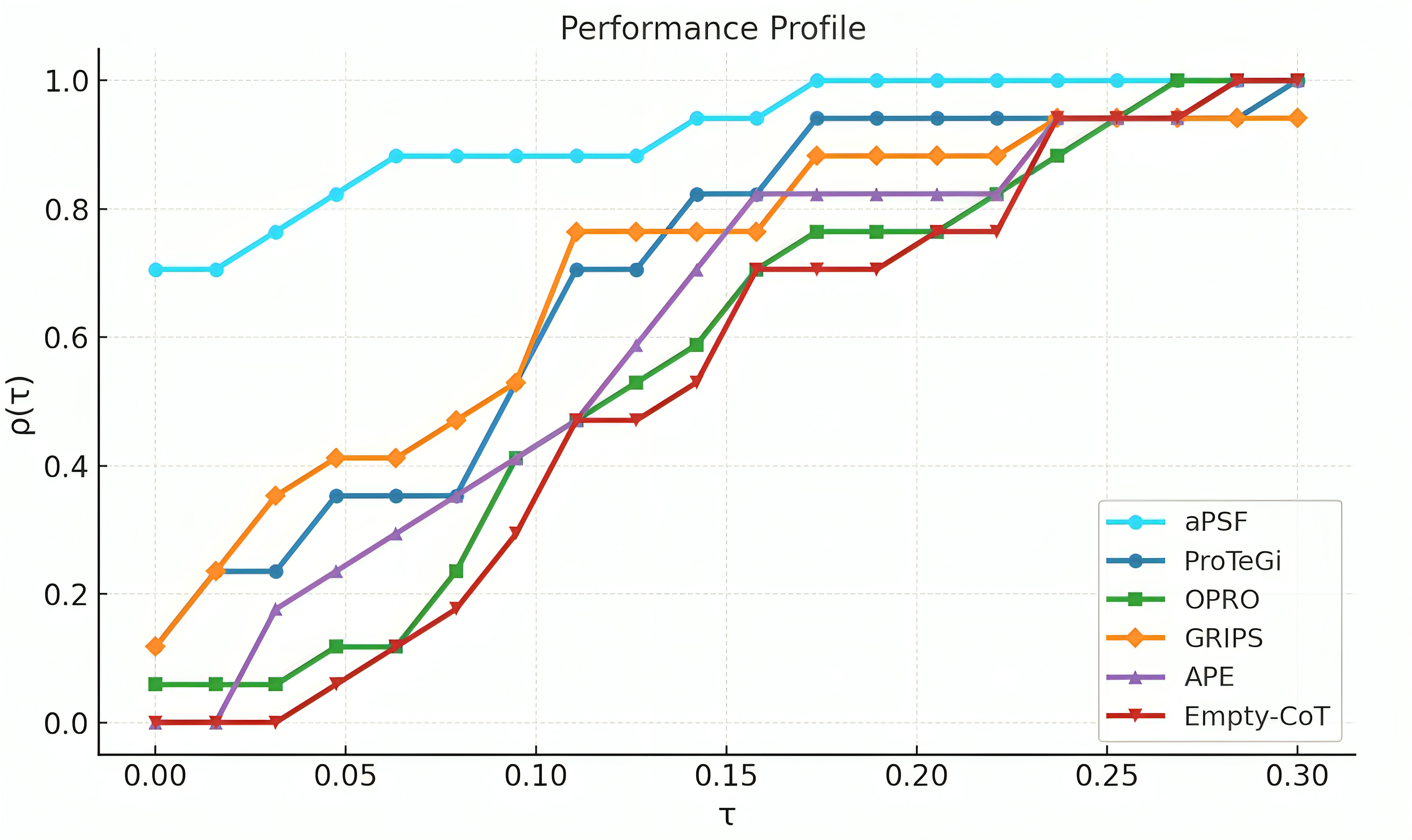## Appendix E Performance Profile Analysis <details> <summary>2604.06699v1/Fig/Performance_Profile.png Details</summary>  ### Visual Description ## Line Chart: Performance Profile ### Overview The chart displays the performance profiles of six algorithms (aPSF, ProTeGi, OPRO, GRIPS, APE, Empty-CoT) across a parameter τ ranging from 0.00 to 0.30. Performance (ρ(τ)) is measured on the y-axis (0.0–1.0), with each algorithm represented by a distinct colored line and marker. All lines exhibit stepwise increases, with performance plateauing at higher τ values. ### Components/Axes - **X-axis (τ)**: Ranges from 0.00 to 0.30 in increments of 0.05. Labeled "τ". - **Y-axis (ρ(τ))**: Performance metric, ranging from 0.0 to 1.0 in increments of 0.2. Labeled "ρ(τ)". - **Legend**: Located in the bottom-right corner, mapping colors to algorithms: - Cyan (○): aPSF - Dark Blue (○): ProTeGi - Green (■): OPRO - Orange (◆): GRIPS - Purple (▲): APE - Red (▼): Empty-CoT ### Detailed Analysis 1. **aPSF (Cyan)**: - Starts at ρ(τ) ≈ 0.7 at τ=0.00. - Increases to ≈0.8 at τ=0.05, then plateaus at ≈0.9 until τ=0.30. - Final value: ρ(τ) ≈ 1.0 at τ=0.30. 2. **ProTeGi (Dark Blue)**: - Begins at ρ(τ) ≈ 0.2 at τ=0.00. - Rises to ≈0.4 at τ=0.05, ≈0.7 at τ=0.10, ≈0.9 at τ=0.15, and plateaus at ≈0.95 until τ=0.30. - Final value: ρ(τ) ≈ 1.0 at τ=0.30. 3. **OPRO (Green)**: - Starts at ρ(τ) ≈ 0.05 at τ=0.00. - Increases to ≈0.2 at τ=0.05, ≈0.5 at τ=0.10, ≈0.75 at τ=0.15, ≈0.85 at τ=0.20, and reaches 1.0 by τ=0.25. - Final value: ρ(τ) ≈ 1.0 at τ=0.30. 4. **GRIPS (Orange)**: - Begins at ρ(τ) ≈ 0.1 at τ=0.00. - Rises to ≈0.4 at τ=0.05, ≈0.8 at τ=0.10, ≈0.85 at τ=0.15, and plateaus at ≈0.9 until τ=0.30. - Final value: ρ(τ) ≈ 0.9 at τ=0.30. 5. **APE (Purple)**: - Starts at ρ(τ) ≈ 0.0 at τ=0.00. - Increases to ≈0.2 at τ=0.05, ≈0.5 at τ=0.10, ≈0.8 at τ=0.15, ≈0.85 at τ=0.20, and reaches 1.0 by τ=0.25. - Final value: ρ(τ) ≈ 1.0 at τ=0.30. 6. **Empty-CoT (Red)**: - Begins at ρ(τ) ≈ 0.0 at τ=0.00. - Rises to ≈0.1 at τ=0.05, ≈0.4 at τ=0.10, ≈0.6 at τ=0.15, ≈0.75 at τ=0.20, and reaches 1.0 by τ=0.25. - Final value: ρ(τ) ≈ 1.0 at τ=0.30. ### Key Observations - **aPSF** maintains the highest performance across all τ values, plateauing near 1.0 early. - **ProTeGi** and **APE** show similar trajectories, with APE surpassing ProTeGi after τ=0.15. - **Empty-CoT** starts the lowest but accelerates sharply, matching aPSF by τ=0.25. - **OPRO** and **GRIPS** exhibit moderate growth, with OPRO outperforming GRIPS after τ=0.10. - All algorithms converge to ρ(τ) ≈ 1.0 by τ=0.30, except GRIPS, which plateaus at ≈0.9. ### Interpretation The chart demonstrates varying algorithm efficiency across τ. aPSF and ProTeGi are top performers, while Empty-CoT shows rapid improvement, suggesting potential for optimization. The convergence of lines at higher τ values implies that performance differences may diminish with increased parameter scaling. GRIPS lags slightly behind others, indicating possible limitations in its design or implementation. The stepwise nature of the lines suggests discrete performance thresholds or algorithmic decision points. </details> Figure 12: Performance profile on BBH sub-tasks. aPSF (red) exhibits the steepest curve and highest plateau, indicating it most frequently achieves near-optimal performance across tasks. At $τ{=}0.1$ (within 10% of best), aPSF succeeds on 76% of tasks vs. 65% for OPRO. Empty-CoT denotes the initial prompt baseline without prompt optimization. Figure 12 shows performance profiles across the 17 BBH sub-tasks we evaluate. The performance profile plots the fraction of tasks where each method achieves accuracy within a factor $τ$ of the best method. aPSF exhibits the steepest curve and highest plateau, indicating it most frequently achieves near-optimal performance. At $τ{=}0.1$ (within 10% of best), aPSF succeeds on 76% of tasks compared to 65% for OPRO, demonstrating superior robustness across diverse reasoning categories. ## Appendix F MMLU Results To evaluate aPSF on knowledge-intensive tasks, we test on MMLU (Hendrycks et al., 2020) (5-shot, 57 subjects). Table 8 shows aPSF achieves the best overall average (76.29%), with strongest improvement on Humanities (+6.18pp) and Other (+1.10pp), though it does not lead in Social Sciences or STEM categories. MMLU Results | Category | aPSF | OPRO | GrIPS | ProTeGi | APE | Zero-shot CoT | $Δ$ vs Best Baseline | | --- | --- | --- | --- | --- | --- | --- | --- | | Humanities | 67.98 | 61.80 | 60.91 | 60.84 | 59.31 | 55.25 | +6.18 | | Social Sciences | 80.04 | 80.70 | 81.19 | 80.34 | 79.94 | 70.83 | -1.15 | | STEM | 76.75 | 77.80 | 77.54 | 77.12 | 75.98 | 66.42 | -1.05 | | Other | 80.37 | 78.60 | 78.35 | 79.27 | 77.08 | 68.91 | +1.10 | | Overall Avg. | 76.29 | 74.72 | 74.50 | 74.39 | 73.08 | 65.35 | +1.57 | Table 8: MMLU accuracy (%) across four disciplinary categories. aPSF achieves best overall average (76.29%) with strongest gains on Humanities (+6.18pp) and Other (+1.10pp), though trailing in Social Sciences and STEM. $Δ$ vs Best Baseline = aPSF’s difference from the strongest non-aPSF baseline in each category (green =aPSF wins, red =aPSF loses). Light blue highlights indicate category winners; purple row emphasizes overall average. ## Appendix G Additional Benchmark Results: GPQA and Competition Math We further evaluate aPSF on scientific reasoning (GPQA (Rein et al., 2024)) and advanced mathematical reasoning (Competition Mathematics (Hendrycks et al., 2021), 500 test samples). Table 9 shows aPSF achieves consistent improvements on these challenging benchmarks. | | aPSF | OPRO | APE | ProTeGi | GrIPS | | --- | --- | --- | --- | --- | --- | | Comp. Math | 56.0 | 51.6 | 54.0 | 54.0 | 55.0 | | GPQA-Chem | 30.2 | 23.8 | 20.6 | 19.1 | 28.6 | | GPQA-Phys | 45.9 | 44.3 | 41.0 | 39.3 | 39.3 | Table 9: Test accuracy (%) on Competition Math and GPQA. Comp. Math = Competition Mathematics; Chem = Chemistry; Phys = Physics. aPSF achieves best on all benchmarks. ## Appendix H Hyperparameter Sensitivity Analysis We evaluate aPSF’s sensitivity to the candidate count $N$ per factor update on the challenging GSM-Hard benchmark. As shown in Table 10, performance does not increase monotonically with $N$ . | Count ( $N$ ) | GSM-Hard (%) | Trend | | --- | --- | --- | | 2 | 52.78 | Under-exploration | | 4 | 54.77 | Optimal Balance | | 6 | 53.88 | Diminishing Returns | | 8 | 50.80 | Overfitting / Noise | Table 10: Sensitivity to candidate count $N$ on GSM-Hard. Performance peaks at $N=4$ , while larger $N$ degrades performance. Analysis: - Under-exploration ( $N=2$ ): Limited candidates fail to uncover effective local edits, resulting in suboptimal performance (52.78%). - Optimal Balance ( $N=4$ ): This setting achieves the peak accuracy (54.77%), effectively balancing exploration width with selection stability. - Overfitting Risk ( $N≥ 6$ ): Contrary to the intuition that “more is better,” increasing $N$ to 8 causes a significant drop to 50.80%. We hypothesize that a larger candidate pool increases the likelihood of finding “false positives” prompts that exploit artifacts in the small validation slice (50 examples) but fail to generalize to the test set. Thus, we adopt $N=4$ as the robust default. ## Appendix I From-Scratch Capability (No Initial Prompt) Our main results use initial-prompt mode (Section 4). Here we evaluate aPSF in from-scratch mode, where the Architect discovers a factorized prompt without any user-provided seed. Table 11 compares the two aPSF modes directly. | Benchmark | aPSF (Initial) | aPSF (Scratch) | $Δ$ | | --- | --- | --- | --- | | GSM-Hard | 54.77 | 54.67 | $-0.10$ | | AQUA-RAT | 82.50 | 83.00 | $+0.50$ | | MultiArith | 99.30 | 99.30 | $± 0.00$ | Table 11: Comparison of aPSF in Initial-Prompt mode (“Let’s think step by step”) vs. From-Scratch mode. Performance is comparable, confirming that aPSF’s gains stem from the factorization mechanism rather than the initial prompt. Key findings. - Comparable performance: The two modes achieve nearly identical results across all three benchmarks, with differences within 0.5pp. This confirms that aPSF’s structure discovery is robust regardless of initialization. - From-scratch can match or exceed: On AQUA-RAT, from-scratch mode slightly outperforms initial-prompt mode (+0.50pp), suggesting that autonomously discovered structures can be as effective as human-guided ones. - Gains not solely from seed: These results confirm that aPSF’s improvements stem from the factorization and optimization mechanism itself, not merely from a privileged starting point. ## Appendix J Complete Factor Selection Statistics Table 12 presents comprehensive factor selection statistics across all evaluated tasks. The test accuracy figures align with the main results reported in Section 4.2. | Task | Test Acc (%) | Val Gain | Gen Gap | Dominant Factor | Selection Rate | | --- | --- | --- | --- | --- | --- | | Mathematical Reasoning: | | | | | | | GSM8K | 90.03 | +0.0% | 0.020 | Result Aggregation | 50% | | AQUA-RAT | 82.50 | +10.3% | 0.035 | Calculation Execution | 50% | | GSM-Hard | 54.77 | +10.3% | 0.102 | Problem Understanding | 67% | | MultiArith | 99.30 | +0.0% | -0.033 | Problem Analysis | 100% | | Logical Reasoning (BBH): | | | | | | | Date Understanding | 80.00 | +12.2% | 0.167 | Time Difference Calc | 100% | | Logical Deduction | 75.00 | +8.6% | 0.013 | Establishing Order | 80% | | Scientific Reasoning (GPQA): | | | | | | | Chemistry | 30.16 | +100% | 0.098 | Reagent Evaluation | 50% | | Physics | 45.90 | +200% | 0.166 | Principle Application | 70% | | Biology | 50.00 | +0.0% | 0.250 | Sci. Principle App. | 50% | | High-Complexity Tasks: | | | | | | | AIME-2025 | 8.33 | +100% | 0.250 | Parse Problem | 50% | Table 12: Complete factor selection statistics across all tasks. Test Acc matches the main results using the default configuration (Qwen2.5-7B-Instruct Worker + Qwen3-8B Architect). Val Gain = validation improvement from initial to best; Gen Gap = difference between validation and test accuracy. Key observations from factor selection patterns. - Task-specific adaptation: Error-guided selection identifies domain-appropriate factors—mathematical tasks often prioritize Calculation or Problem Understanding, logic tasks focus on Step-by-Step reasoning, and scientific tasks emphasize Principle Application. - Selection Concentration: Tasks with 100% selection on a single factor indicate two distinct states: saturation (e.g., MultiArith, +0.0% gain) where the initial prompt is already optimal, or critical bottlenecking (e.g., BBH-Date, +12.2% gain) where one specific skill dictates performance. 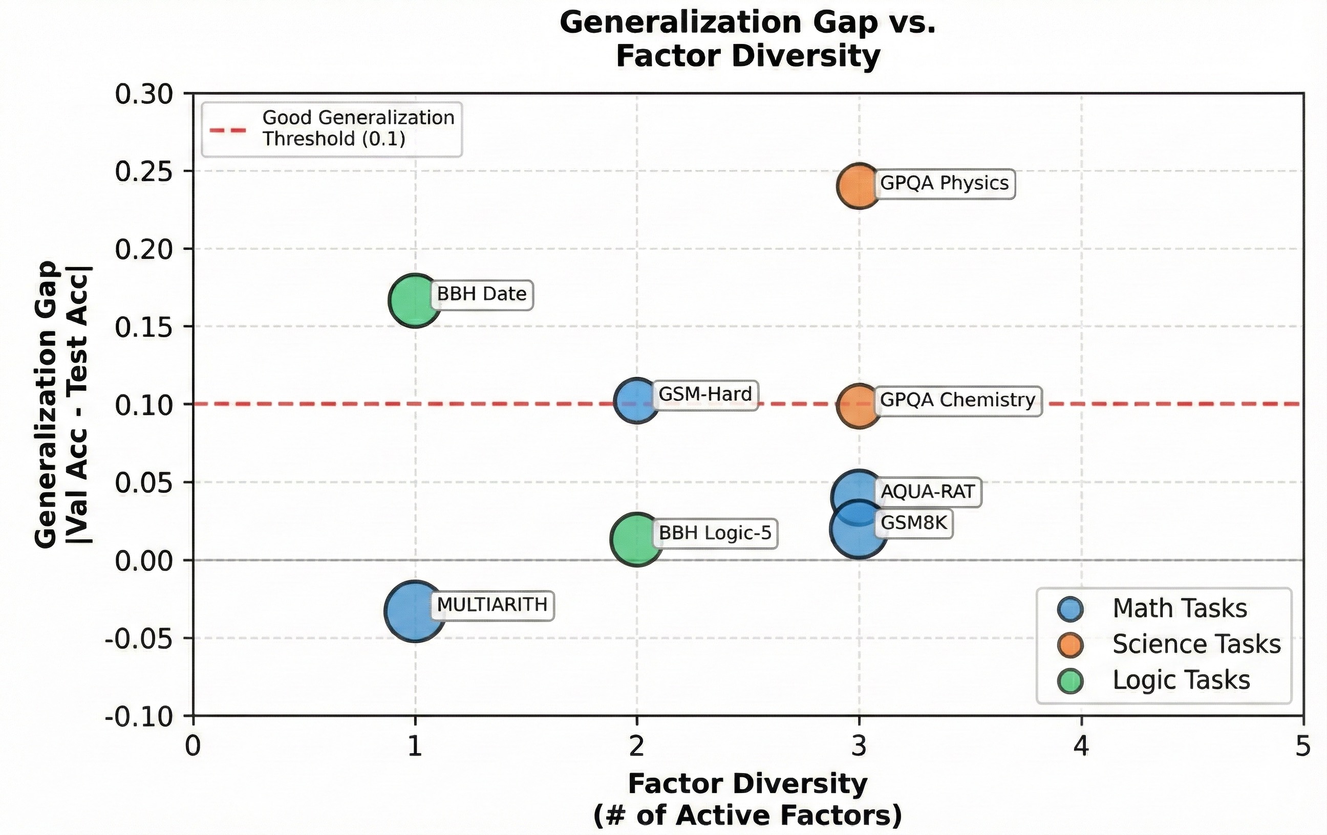<details> <summary>2604.06699v1/Fig/edited-image.png Details</summary>  ### Visual Description ## Scatter Plot: Generalization Gap vs. Factor Diversity ### Overview The chart visualizes the relationship between **Factor Diversity** (number of active factors) and **Generalization Gap** (absolute difference between validation accuracy and test accuracy) across three task categories: Math, Science, and Logic. A red dashed line at 0.1 marks the "Good Generalization Threshold." ### Components/Axes - **X-axis**: Factor Diversity (# of Active Factors) – ranges from 0 to 5. - **Y-axis**: Generalization Gap |(Val Acc - Test Acc)| – ranges from -0.10 to 0.30. - **Legend**: - Blue: Math Tasks - Orange: Science Tasks - Green: Logic Tasks - **Threshold Line**: Red dashed line at y = 0.1. ### Detailed Analysis 1. **Math Tasks (Blue)**: - **MULTIARITH**: (1, -0.05) – below threshold. - **GSM-Hard**: (2, 0.10) – on threshold. - **AQUA-RAT**: (3, 0.04) – below threshold. - **GSM8K**: (3, 0.03) – below threshold. 2. **Science Tasks (Orange)**: - **GPQA Chemistry**: (3, 0.10) – on threshold. - **GPQA Physics**: (3.5, 0.24) – well above threshold. 3. **Logic Tasks (Green)**: - **BBH Logic-5**: (2, 0.00) – on threshold. - **BBH Date**: (1, 0.16) – above threshold. ### Key Observations - **Highest Generalization Gap**: GPQA Physics (0.24) – Science Task with 3.5 active factors. - **Lowest Generalization Gap**: MULTIARITH (-0.05) – Math Task with 1 active factor. - **Threshold Crossings**: - 3 tasks (GSM-Hard, GPQA Chemistry, BBH Logic-5) meet/exceed the 0.1 threshold. - 5 tasks fall below the threshold, including GPQA Physics despite high factor diversity. ### Interpretation The data suggests that **Factor Diversity does not consistently correlate with Generalization Gap**. While Science Tasks (e.g., GPQA Physics) often exhibit larger gaps, some Math and Logic Tasks (e.g., GSM8K, BBH Logic-5) achieve near-zero gaps even with fewer factors. The threshold line highlights that only a minority of tasks meet the "Good Generalization" criterion, emphasizing the need for task-specific optimization strategies. Notably, GPQA Physics’s high gap despite 3.5 factors challenges the assumption that increased complexity inherently improves generalization. </details> Figure 13: Generalization Gap vs. Factor Diversity. Visualizing the relationship between factor count and generalization gap (data from Table 12). Robust tasks (e.g., GSM8K, AQUA) maintain low gaps ( $<0.05$ ) with balanced factors. High gaps in complex tasks (e.g., GPQA) reflect intrinsic difficulty rather than optimization overfitting. - Generalization quality: As visualized in Figure 13, tasks with balanced factor distributions (20–50% each) exhibit lower generalization gaps (GSM8K: 0.020, AQUA: 0.035), whereas concentrated or high-complexity tasks correlate with higher gaps (AIME: 0.250). - Validation-test alignment: High validation gains (+100–200%) on challenging tasks (GPQA-Physics, AIME) indicate effective optimization, confirming that the framework can exploit headroom even when absolute accuracy remains limited by task difficulty. ## Appendix K Detailed Factor Names by Task Table 13 presents the original, task-specific factor names discovered by aPSF’s Architect LLM. | Task | Discovered Factor Names (Original) | Top Factor (Rate) | | --- | --- | --- | | Mathematical Reasoning: | | | | GSM8K | StepByStepDecomposition, ComponentAnalysis, CalculationExecution, ResultAggregation | ResultAggregation (50%) | | AQUA-RAT | StepByStepReasoning, ProblemAnalysis, StepBreakdown, CalculationExecution, Verification, AnswerSelection | CalculationExecution (50%) | | GSM-Hard | ProblemUnderstanding, StepByStepBreakdown, MathematicalOperations, FinalCalculation, Verification | ProblemUnderstanding (67%) | | MultiArith | StepByStepApproach, ProblemAnalysis, SequentialExecution, ResultValidation | ProblemAnalysis (100%) | | Logical Reasoning (BBH): | | | | Date Understanding | StepByStepApproach, DateParsing, TimeDifferenceCalculation, CalendarRuleApplication, OptionVerification | TimeDifferenceCalculation (100%) | | Logical Deduction | ParsingStatements, EstablishingOrder, EvaluatingOptions | EstablishingOrder (80%) | | Scientific Reasoning (GPQA): | | | | Chemistry | ReactionAnalysis, ReagentEvaluation, ProductStability, StereochemistryConsideration, OptionElimination | ReagentEvaluation (50%) | | Physics | ContextAnalysis, ParameterExtraction, PrincipleApplication, CalculationExecution, ValidationCheck | PrincipleApplication (70%) | | Biology | ContextualInterpretation, ScientificPrincipleApplication, OptionEvaluation, Elimination&Justification | Sci. Principle App. (50%) | | High-Complexity Tasks: | | | | AIME-2025 | ParseProblem, IdentifyConcepts, BreakSubproblems, StepwiseReasoning, ValidateSteps, SynthesizeResults | ParseProblem (50%) | Table 13: Original factor names autonomously discovered by aPSF. The terminology adapts to the domain (e.g., Stereochemistry in Chemistry, CalculationExecution in AQUA). Top Factor indicates the component most frequently selected by the error-guided scheduler. Semantic grouping for cross-task analysis. For the heatmap visualization in Figure 4 (main text), we semantically group task-specific factors into six general categories to enable cross-task pattern comparison: (i) Problem Understanding (e.g., ProblemAnalysis, ComponentAnalysis, ParsingStatements), (ii) Step-by-Step Breakdown (e.g., EstablishingOrder, StepByStepBreakdown), (iii) Mathematical Operations (e.g., MathematicalOperations, FormulaUsage), (iv) Calculation Execution (e.g., CalculationExecution, TimeDifferenceCalculation), (v) Verification & Validation (e.g., Verification, ResultValidation), and (vi) Result Aggregation (e.g., ResultAggregation, AnswerSelection, LogicalDeduction). This grouping preserves semantic intent while enabling macro-level pattern analysis across diverse task domains. ## Appendix L Factor Discovery Examples This section provides concrete examples of discovered factor structures and illustrates the prompt transformation process. #### L.0.1 Initial-Prompt Mode Extension Example Starting from the baseline “Let’s think step by step” on GSM8K, the Architect LLM analyzes the reasoning style and generates the following extension: Extended Instruction: “Let’s think step by step, carefully analyzing the problem’s components and their relationships, performing each calculation with clear intermediate steps, and logically combining all results to arrive at the final answer.” The system then decomposes this into independently optimizable factors: - $F_1$ -StepByStepDecomposition: “Let’s think step by step” - $F_2$ -ComponentAnalysis: “carefully analyzing the problem’s components and their relationships” - $F_3$ -CalculationExecution: “performing each calculation with clear intermediate steps” - $F_4$ -ResultAggregation: “logically combining all results to arrive at the final answer” This demonstrates how aPSF preserves the core reasoning style while injecting task-specific procedural guidance, enabling subsequent factor-wise optimization. #### L.0.2 BBH–Logical Deduction: A Complete Optimization Trace We present a complete example on BBH–Logical Deduction (Five Objects), a task requiring constraint parsing, order establishment, and option verification. Starting from the same initial prompt baseline (Zero-shot): Initial Prompt: “Let’s think step by step.” The Architect LLM analyzes the task requirements (parsing comparative statements like “A is before B”, building a global ordering chain) and generates: Extended Instruction: “Carefully read the given statements and identify all comparative relationships between the items. Use these relationships to create a logical order of the items from highest to lowest. Then, evaluate each option against this order to determine which one is correct. When establishing the order, build the sequence incrementally by validating each comparative relationship against the current order and explicitly confirming chains of relationships (e.g., A < B < C) step by step to prevent logical gaps.” The system decomposes this into three semantic factors: - $F_1$ -ParsingStatements: “Carefully read the given statements and identify all comparative relationships between the items.” - $F_2$ -EstablishingOrder: “Use these relationships to create a logical order… build the sequence incrementally by validating each comparative relationship…” - $F_3$ -EvaluatingOptions: “Evaluate each option against this order to determine which one is correct.” Error-guided optimization results. During optimization, error analysis reveals that 80% of failures stem from incorrect order establishment (e.g., missing transitive relationships, premature chain termination). The error-guided selector consequently prioritizes $F_2$ -EstablishingOrder across 8 of 10 optimization rounds. Key metrics: | Metric | Value | | --- | --- | | Initial validation accuracy | 70.0% | | Best validation accuracy | 76.0% | | Final test accuracy | 74.67% | | Validation improvement | +8.6% | | Generalization gap | 0.013 (excellent) | | Dominant factor | EstablishingOrder (80%) | This example illustrates how aPSF automatically identifies task-specific bottlenecks and focuses optimization effort accordingly. #### L.0.3 Discovered Factor Structures by Task Type Table 14 presents concrete factor structures autonomously discovered by aPSF for diverse task types, illustrating adaptive factorization based on task complexity. Note that factor names align with the terminology identified in Table 13. | Task Type | Discovered Factors | Order | | --- | --- | --- | | Math (GSM8K) | 1. StepByStepDecomposition: Decompose problem step by step 2. ComponentAnalysis: Identify key quantities 3. CalculationExecution: Perform arithmetic operations 4. ResultAggregation: Format final output | $1→ 2→ 3→ 4$ | | Logic (BBH) | 1. ParsingStatements: Extract logical premises 2. EstablishingOrder: Deduce chronological/logical sequence 3. EvaluatingOptions: Verify consistency against premises 4. OptionVerification: Double-check constraints | $1→ 2→ 3→ 4$ | | QA (AQUA) | 1. ProblemAnalysis: Identify question type 2. CalculationExecution: Perform systematic calculations 3. Verification: Self-validate plausibility 4. AnswerSelection: Select correct option | $1→ 2→ 3→ 4$ | Table 14: Factor structures discovered by aPSF. The factor names (e.g., ComponentAnalysis, CalculationExecution) correspond to the domain-specific terminology cataloged in Appendix K. ## Appendix M Theoretical Analysis We provide a formal intuition for why aPSF’s error-guided factor selection outperforms fixed schedules, focusing on regret minimization under non-stationary rewards. ### M.1 Problem Formulation We view prompt optimization as a sequential decision process. At step $t$ , the Architect chooses a factor $k∈\{1,\dots,K\}$ to optimize. Let $μ_k^(t)$ be the potential improvement gain of factor $k$ at time $t$ . The cumulative regret after $T_\max$ steps is: $$ R(T_\max)=∑_t=1^T_\max\max_k(μ_k^(t))-∑_t=1^T_\maxμ_k_{t}^(t), \tag{10} $$ where $\max_k(μ_k^(t))$ is the gain of the optimal action (Oracle). ### M.2 Why Error-Guided Factor Selection Wins Fixed policies (Round-robin). A round-robin policy selects $k$ uniformly, ignoring the current state. If factor potentials are heterogeneous (e.g., Format is broken while Instruction is perfect), fixed policies waste $1-1/K$ of the budget on saturated factors, leading to linear regret. Error-Guided Factor Selection as Contextual Bandits. Our Error-Guided factor selection policy $π$ observes the current error distribution $E^(t)$ (Context) to select action $k$ . Under the assumption that the Architect’s diagnosis accuracy is $ρ>1/K$ , the policy prioritizes high-potential factors (e.g., fixing Format when format errors are high). This effectively creates a shortcut to convergence: $$ E_π[gain]≈ρ·μ_bottleneck^(t)+(1-ρ)·\bar{μ}^(t). \tag{11} $$ By focusing on the bottleneck, $R(T_\max)$ is minimized significantly faster than round-robin, consistent with the rapid convergence observed in the trajectory analysis (Figure 14 in Appendix S). ### M.3 Independence Assumption and Complexity aPSF optimizes factors iteratively (Coordinate Descent), assuming partial independence: $\hat{S}(A∪ B)≈\hat{S}(A)+\hat{S}(B)$ . While subtle factor interactions naturally exist (e.g., between reasoning steps and formatting constraints), modeling the full joint distribution would result in an exponential search space $O(C^K)$ (where $C$ is the candidate count). By adopting the independence assumption, aPSF reduces the complexity to linear $O(C· K· T_\max)$ . This trade-off makes optimization tractable for LLMs, as demonstrated by the strong empirical results across diverse benchmarks. ### M.4 Convergence Properties Under Interventional Updates Note: This section provides informal convergence arguments rather than rigorous proofs. Let $B^(t)$ denote the factor contents at iteration $t$ , and $\hat{S}^(t)=\hat{S}(Assemble(B^(t)),D_val)$ be the validation accuracy. aPSF’s update rule is: $$ f_k^(t+1)=\begin{cases}\hat{c}_k&if Δ\hat{S}(\hat{c}_k)≥δ\\ f_k^(t)&otherwise\end{cases}, \tag{12} $$ where $\hat{c}_k$ is the best candidate proposed by the Architect $M_A$ , and $δ>0$ is the acceptance threshold. Monotonicity. By construction, $\hat{S}^(t+1)≥\hat{S}^(t)$ (non-decreasing accuracy). Unlike non-contrastive methods that evaluate the whole prompt blindly, aPSF accepts updates only if the isolated marginal contribution $Δ\hat{S}≥δ$ . This strictly prevents regressions caused by noisy edits. Convergence Intuition. Assuming a bounded factor space and a capable Architect $M_A$ that generates diverse candidates, the system performs a hill-climbing search (Coordinate Descent). Since the objective function is bounded ( $\hat{S}∈[0,1]$ ) and the sequence is non-decreasing, the optimization is expected to converge to a local maximum where no single-factor edit yields improvement $≥δ$ . ### M.5 Information-Theoretic Justification Let $E^(t)$ denote the distribution of validation errors at step $t$ (e.g., 40% Arithmetic, 10% Format). Information-Theoretic Intuition. Ideally, we want to select the factor $k$ whose edits are most informative about (and most likely to reduce) the current error modes. Formally, this corresponds to maximizing mutual information $I(F_k;E^(t))$ between factor $k$ and the error distribution. We do not estimate mutual information explicitly; instead, our Error-Guided Factor Selection approximates this criterion by using the Architect LLM to diagnose which factor is causally linked to the dominant error types. Connection to Contextual Bandits. Standard prompt optimizers (like OPRO) often behave like Multi-Armed Bandits (MAB), exploring factors to maximize reward. However, standard MAB assumes stationary rewards. In prompt engineering, rewards are non-stationary (fixing the Instruction changes the utility of fixing Examples). aPSF treats this as a Contextual Bandit problem: - Context: Current error distribution $E^(t)$ . - Action: Select factor $k$ . - Policy: The Architect maps context (e.g., "Format Error") to action (e.g., "Fix Factor 4"). This contextual awareness allows aPSF to "exploit" known bottlenecks immediately, rather than wasting steps "exploring" saturated factors. This explains the rapid convergence observed in the trajectory analysis (Figure 14 in Appendix S). ## Appendix N Model Configurations ### N.1 LLM Specifications To ensure reproducibility and accessibility, we primarily utilize high-performance open-weight models. We distinguish between two roles: Worker Models ( $M_W$ ). The worker executes the task based on the assembled prompt. We evaluate two families: - Qwen2.5-7B-Instruct: This is a 7B parameter instruction-tuned model, context window up to 32K tokens, quantization: FP16. - Llama-3.1-8B-Instruct: This is an 8B parameter instruction-tuned model, context window up to 128K tokens, quantization: FP16. Architect LLM ( $M_A$ ). The architect handles structure discovery, factor editing, and error diagnosis. We employ stronger models for these meta-reasoning tasks: - Qwen3-8B: Used as the default Architect for most experiments due to its strong instruction-following capability. - gpt-oss-120b: A large-scale open-source model used in ablation studies to verify scalability. Accessed via API with temperature=0.7. ### N.2 Decoding Hyperparameters All inference uses the settings detailed in Table 15, unless explicitly varied. | Parameter | Value | | --- | --- | | Temperature | 0.0 (deterministic) | | Top-p (nucleus sampling) | 1.0 (disabled) | | Top-k | Not applied | | Max output tokens | 8192 | | Repetition penalty | 1.0 (disabled) | | Stop sequences | ["\n\n", "---"] | Table 15: Decoding hyperparameters for Worker model inference ( $M_W$ ). These settings apply to both prompt selection on $D_val$ and final test evaluation. For the Architect LLM ( $M_A$ ) generating meta-level content (e.g., structure proposals, factor edits), we use temperature=0.7 to encourage diversity while maintaining coherence. Summary of Temperature Settings. Worker ( $M_W$ ): temperature=0.0 (deterministic) for all inference, including both prompt selection and final test evaluation. Architect ( $M_A$ ): temperature=0.7 to encourage diverse structure proposals. ## Appendix O Evaluation Protocol ### O.1 Data Splitting For each benchmark, we utilize a small, fixed validation slice ( $|D_val|=50$ examples) for prompt optimization and a held-out test set for final evaluation, as detailed in Table 16: | Dataset | Validation Slice | Test Size | | --- | --- | --- | | GSM8K | 50 | 1,319 | | AQUA-RAT | 50 | 254 | | MultiArith | 50 | 180 | | GSM-Hard | 50 | 1006 | | BBH (per task) | 50 | Variable | Table 16: Dataset splits. We use a fixed validation slice of 50 examples per task for prompt optimization. Test sets follow official benchmarks where available. ### O.2 Scoring Functions Math benchmarks (GSM8K, AQUA, MultiArith, GSM-Hard). We use exact-match accuracy: extract the final numerical answer using regex patterns (e.g., “The answer is \d+”), normalize to remove commas/units, and compare string equality with ground truth. BBH and complex reasoning benchmarks. For tasks with diverse answer formats (e.g., Yes/No, multiple choice A–E, or free-form text), we use LLM-based answer extraction: a lightweight LLM extracts the final answer from model outputs, which is then compared against ground truth for exact-match accuracy. This approach handles varied response formats more robustly than regex patterns. ## Appendix P Computational Resources All experiments run on the following infrastructure: - GPUs: 2 $×$ NVIDIA A100 80GB GPUs for worker inference - CPU: 64-core AMD EPYC 7763 @ 2.45GHz - RAM: 512GB DDR4 - OS: Ubuntu 20.04 LTS, CUDA 11.8, PyTorch 2.0.1 ## Appendix Q Datasets and Licenses We summarize the benchmarks, task types, split sources, and license details in Table 17. and include the following information for reproducibility: - Download URLs: Provided in code release README. - Preprocessing: Scripts for answer normalization and format extraction are included in the supplementary material. - Version Control: Pinned commit hashes are used to ensure reproducibility. Table 17: Summary of evaluation benchmarks. All datasets are publicly available. ## Appendix R Implementation Details ### R.1 Prompt Assembly Factors are concatenated in the specified order via the $Assemble$ operation (Eq. 3), separated by newlines for readability. Total prompt length is implicitly bounded by the worker LLM’s context window (up to 32K tokens for Qwen2.5 per official configuration); in practice, generated prompts rarely approach this limit. ### R.2 Validation Slice Design We use a fixed per-task validation slice for prompt optimization (Appendix O). ### R.3 Stopping Criteria aPSF terminates when: (i) $T_\max$ iterations are reached, or (ii) validation performance has not improved for 3 consecutive iterations (early stopping). ### R.4 Prompt Length Sensitivity Analysis Prior work has shown that smaller language models are sensitive to prompt length (Wei et al., 2022). To validate this, we conducted ablation studies on prompt length using Llama-3.1-8B-Instruct (to test generalization beyond our default Qwen model). Table 18 shows a clear inverse relationship between prompt length and accuracy on GSM8K. | Prompt Length (tokens) | Accuracy (%) | | --- | --- | | 362 | 89.62 | | 500 | 83.50 | | 653 | 80.55 | | 1260 | 76.47 | Table 18: Impact of prompt length on Llama-3.1-8B-Instruct performance (GSM8K). Accuracy degrades significantly as prompts exceed 500 tokens. These findings suggest that prompt conciseness is particularly important for smaller models. In our main experiments, we do not impose explicit length constraints in the meta-prompts, allowing the Architect LLM to generate prompts of varying lengths; the factor-wise optimization naturally tends to retain concise, effective phrasings through performance-based selection. ### R.5 Extended Efficiency Analysis We extend the efficiency analysis from MultiArith (Section 4.4) to four datasets. Table 19 reports the token consumption at the best validation step and the step number itself, under the default setup (Worker: Qwen2.5-7B-Instruct; Architect: Qwen3-8B). | Method | Tokens at Best Step (K) | | | | | --- | --- | --- | --- | --- | | MultiArith | GSM8K | AQUA | GSM-Hard | | | ProTeGi | 1455 | 2143 | 1896 | 2850 | | GrIPS | 1640 | 1932 | 1968 | 2378 | | CriSPO | 1050 | 1612 | 1644 | 2268 | | APE | 824 | 1206 | 948 | 1445 | | ZERA | 460 | 910 | 529 | 1148 | | OPRO | 377 | 850 | 593 | 1110 | | aPSF | 206 | 491 | 336 | 648 | | Method | Best Step ( $↓$ ) | | | | | --- | --- | --- | --- | --- | | MultiArith | GSM8K | AQUA | GSM-Hard | | | GrIPS | 10 | 9 | 10 | 10 | | ProTeGi | 7 | 8 | 8 | 10 | | CriSPO | 5 | 6 | 7 | 8 | | APE | 6 | 7 | 6 | 8 | | ZERA | 3 | 5 | 3 | 6 | | OPRO | 2 | 4 | 3 | 5 | | aPSF | 1 | 3 | 2 | 4 | Table 19: Extended efficiency analysis across four datasets. Top: Token consumption (K) at the best validation step. Bottom: Best step number (lower = faster convergence). aPSF consistently reaches peak validation with the fewest tokens and earliest steps. aPSF reaches peak validation with 36–55% fewer tokens than OPRO and ZERA across all datasets, confirming that the efficiency gains observed on MultiArith generalize broadly. ## Appendix S Optimization Trajectory Analysis We analyze the step-wise optimization process on the BBH Date Understanding task. Figure 14 illustrates the validation accuracy trajectory over 30 steps. 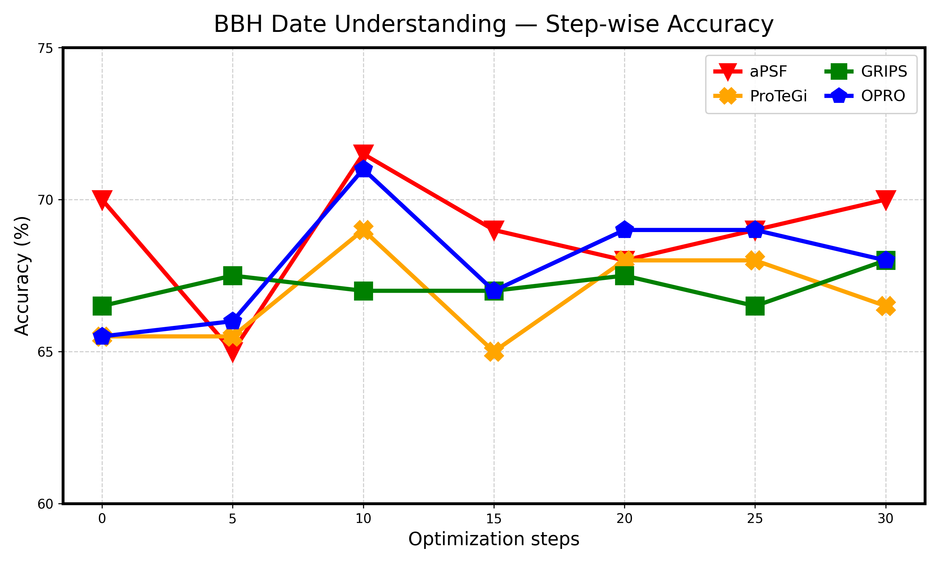<details> <summary>2604.06699v1/Fig/bbh_date_stepwise.png Details</summary>  ### Visual Description ## Line Chart: BBH Date Understanding — Step-wise Accuracy ### Overview The chart visualizes the accuracy trends of four algorithms (aPSF, GRIPS, ProTeGi, OPRO) across 30 optimization steps. Accuracy is measured in percentage, with values ranging from 60% to 75%. Each algorithm is represented by a distinct line and marker type, with trends showing variability in performance over steps. ### Components/Axes - **X-axis**: "Optimization steps" (0 to 30, increments of 5). - **Y-axis**: "Accuracy (%)" (60% to 75%, increments of 5%). - **Legend**: Located in the top-right corner, mapping colors/markers to algorithms: - Red triangles: aPSF - Green squares: GRIPS - Yellow crosses: ProTeGi - Blue diamonds: OPRO ### Detailed Analysis 1. **aPSF (Red Triangles)**: - Starts at ~70% (step 0), drops to ~65% (step 5), peaks at ~72% (step 10), then declines to ~68% (step 15), stabilizes at ~67% (step 20), rises to ~68% (step 25), and ends at ~70% (step 30). - **Trend**: V-shaped with a peak at step 10. 2. **GRIPS (Green Squares)**: - Starts at ~66% (step 0), rises to ~67% (step 5), remains stable (~67%) until step 10, dips to ~66.5% (step 15), increases to ~67.5% (step 20), drops to ~66.5% (step 25), and ends at ~67.5% (step 30). - **Trend**: Relatively flat with minor fluctuations. 3. **ProTeGi (Yellow Crosses)**: - Starts at ~65.5% (step 0), drops to ~65% (step 5), peaks at ~68.5% (step 10), plunges to ~65% (step 15), rises to ~67.5% (step 20), stabilizes at ~67.5% (step 25), and ends at ~66.5% (step 30). - **Trend**: Sharp dip at step 15, followed by recovery. 4. **OPRO (Blue Diamonds)**: - Starts at ~65.5% (step 0), rises to ~66% (step 5), peaks at ~71% (step 10), declines to ~66.5% (step 15), increases to ~68.5% (step 20), stabilizes at ~68.5% (step 25), and ends at ~67.5% (step 30). - **Trend**: Sharp rise to step 10, followed by volatility. ### Key Observations - **aPSF** and **OPRO** exhibit the highest accuracy peaks (~72% and ~71%, respectively) at step 10. - **ProTeGi** shows the lowest accuracy (~65%) at step 15, indicating a significant dip. - **GRIPS** maintains the most stable performance, with minimal fluctuations (~66–67.5%). - All algorithms converge toward ~67–68% accuracy by step 30, except **aPSF**, which recovers to ~70%. ### Interpretation The data suggests that **aPSF** and **OPRO** perform optimally in early optimization steps (peaking at step 10), while **ProTeGi** struggles with a mid-step decline. **GRIPS** demonstrates consistent reliability, making it a stable choice. The convergence of accuracies by step 30 implies diminishing returns or stabilization in later steps. The sharp dip in **ProTeGi** at step 15 may indicate sensitivity to specific optimization conditions. Overall, the chart highlights trade-offs between early performance gains and long-term stability across algorithms. </details> Figure 14: Step-wise optimization trajectory on BBH Date Understanding. aPSF (red) achieves the highest peak accuracy ( $>$ 71% at Step 10) and maintains a leading position by Step 30. In contrast, monolithic methods like OPRO (blue) and ProTeGi (orange) exhibit higher volatility or lower convergence ceilings. Extended-budget analysis (30 steps) for visualization only; main results use $T_\max=10$ . All methods use the same extended budget. Key Observation: aPSF demonstrates rapid convergence, reaching its peak performance early (Step 10). The acceptance threshold $δ$ ensures monotonic progress on validation accuracy—rejected candidates cause plateau periods (e.g., Steps 5–8) rather than regressions. The error-guided mechanism then identifies productive factors to resume improvement, ultimately stabilizing at a higher accuracy level than baselines like GrIPS (Green) or ProTeGi. Step 1: Error Diagnosis (Snapshot) The Architect analyzes validation failures and maps them to specific factors. [Sample 7] Error: Misinterpreted algebraic expression. $→$ Factor1_UnderstandProblem (Conf: 0.92) [Sample 11] Error: Incorrect probability independence assumption. $→$ Factor2_SolveProblem (Conf: 0.92) [Sample 31] Error: Output lengthy explanation instead of single letter. $→$ Factor4_OutputAnswer (Conf: 0.93) [Sample 43] Error: Used incorrect LCM method for rate problem. $→$ Factor2_SolveProblem (Conf: 0.93) … (analyzed 15 error samples in total) Step 2: Aggregation & Selection The system aggregates error counts to identify the critical bottleneck. • Factor1_UnderstandProblem: 3 errors (20.0%) • Factor2_SolveProblem: 6 errors (40.0%) $←$ SELECTED BOTTLENECK • Factor3_SelectChoice: 3 errors (20.0%) • Factor4_OutputAnswer: 3 errors (20.0%) Decision: Prioritize optimizing Factor2_SolveProblem due to highest error frequency. Step 3: Candidate Generation The Architect generates targeted refinements for Factor 2. Old Factor 2: "Solve the problem step by step." New Candidates: 1. "Work through the problem methodically, applying relevant concepts and checking equations…" 2. "Solve the problem by clearly stating the needed formulas, performing calculation…" 3. "Break the question into parts, apply appropriate reasoning, compute intermediate…" 4. "Use step-by-step deduction: identify givens, apply relevant rules, simplify, and…" Figure 15: Real-world execution trace of the Error-Guided Factor Selection mechanism. The system identifies that 40% of errors stem from reasoning flaws (SolveProblem), correctly prioritizing it over format or understanding issues for this iteration. ## Appendix T Qualitative Analysis: Success and Failure Cases Case 1: Integer Constraints on Quadratics (Sample 48) [Success] Demonstrates rigorous algebraic manipulation and case enumeration. Question: For how many integer values of $a$ does the equation $x^2+ax+5a=0$ have integer solutions for $x$ ? aPSF Derivation (Summary): 1. Applied Vieta’s formulas: $p+q=-a,pq=5a$ . 2. Derived the factorization equation: $pq+5p+5q+25=25\implies(p+5)(q+5)=25$ . 3. Enumerated all factor pairs of 25: $(1,25),(-1,-25),(5,5),(-5,-5),(25,1),(-25,-1)$ . 4. Solved for $a$ in each case and filtered distinct values: $\{-16,36,0,20\}$ . aPSF Answer: $4$ Ground Truth: 4 ✓ Analysis: The structured prompt successfully guided the model to perform a variable transformation and exhaustive enumeration without hallucinating invalid pairs. Case 2: Complex Roots of Unity (Sample 49) [Success] Demonstrates handling of complex number properties and polynomial coefficients. Question: Let $ω^7=1,ω≠ 1$ . $α=ω+ω^2+ω^4$ , $β=ω^3+ω^5+ω^6$ . Find $(a,b)$ for $x^2+ax+b=0$ . aPSF Derivation (Summary): 1. Identified property $∑_k=0^6ω^k=0\implies∑_k=1^6ω^k=-1$ . 2. Calculated sum: $α+β=∑_k=1^6ω^k=-1\implies a=-(sum)=1$ . 3. Calculated product: $αβ=(ω+ω^2+ω^4)(ω^3+ω^5+ω^6)$ . Expanded terms and simplified using $ω^7=1$ to find $αβ=2\implies b=2$ . aPSF Answer: $(1, 2)$ Ground Truth: (1, 2) ✓ Analysis: The decomposition allowed the model to maintain clarity during the complex expansion of $αβ$ , correctly identifying it as a sum of specific roots plus an integer. Case 3: Nested Complex Functions (Sample 47) [Failure] Demonstrates limitation in handling high-complexity functional composition. Question: Let $f(z)=\frac{z+a}{z+b},|a|=1$ . If $g(z)=f(f(z))$ and $g(g(z))=z$ , find the difference between max and min values of $|b|$ . aPSF Derivation (Summary): 1. Correctly attempted to expand $g(z)=f(f(z))$ and $g(g(z))$ . 2. The algebraic expansion of the fourth-order composition $g(g(z))$ became overly complex. 3. Incorrectly simplified the condition to a rotation argument ( $f(z)$ must be a rotation by $±π/2$ ), concluding $|b|=1$ and difference is 0. aPSF Answer: $0$ Ground Truth: $√{3}-1$ ✗ Analysis: While the prompt structure enforced step-by-step derivation, the sheer algebraic complexity of expanding a nested Möbius transformation overwhelmed the model’s context tracking, leading to a hallucinatory simplification. This suggests a need for a specialized ToolUse factor (e.g., SymPy) for such tasks. Figure 16: Qualitative comparison of reasoning traces. Cases 1 & 2 show aPSF’s ability to handle structured algebraic and number-theoretic reasoning. Case 3 highlights a failure mode where extreme algebraic complexity leads to incorrect simplification, pointing to future directions for tool-augmented factors. We analyze three representative samples (two successes, one failure) from the evaluation logs to illustrate the reasoning capabilities and limitations of aPSF. Figure 16 presents the detailed breakdown. ## Appendix U Limitations and Future Work ### U.1 Current Limitations Architect quality dependency. aPSF’s factorization quality depends on the Architect LLM’s capability. Weaker architects may: - Propose redundant factors (e.g., separate “Instruction” and “Task Description”) - Under-discover useful factors (missing Format/Verifier on structured tasks) - Create overlapping factor boundaries (non-orthogonal decomposition) Changing the Architect model can affect performance (Table 1). Interventional scoring underestimates synergy. By isolating single-factor updates, interventional factor-level scoring may miss joint improvements where two factors help only in combination (e.g., synergy between Examples and Rationale). Future work could explore block-wise joint edits for factor pairs with high interaction. LLM-based error diagnosis. Error-Guided selection relies on an LLM to analyze step-level errors and map them to factors. While empirically effective (Table 4), diagnostic quality depends on the LLM’s reasoning capability and may introduce noise or bias. Future work could explore hybrid approaches combining error-pattern matching with learned factor-error associations. Hyperparameter sensitivity. Performance can vary with the acceptance threshold $δ$ and candidate count $N$ ; we use $δ{=}1/|D_val|$ and $N{=}4$ by default (see Section 4). Sensitivity analysis is provided in Appendix H. Text-only reasoning benchmarks. Our evaluation focuses on math and logical reasoning tasks with textual I/O. Generalization to: - Multimodal tasks: Vision-language tasks may require different factor types (e.g., ImageGuidance) - Tool-augmented settings: Code execution or API calls may need ToolSelection and ErrorHandling factors - Long-context tasks: Summarization/QA over long documents may benefit from ChunkingStrategy factors ### U.2 Future Directions Adaptive candidate count. Currently $N{=}4$ candidates per update for all factors. Future work could adjust $N$ based on factor type (e.g., $N{=}8$ for Examples, $N{=}2$ for Format) or factor saturation (reduce $N$ after error analysis indicates diminishing returns). Hierarchical factorization. Complex tasks may benefit from hierarchical factor structures (e.g., Rationale $→$ {PlanningStep, ExecutionStep, VerificationStep}). Extending aPSF to multi-level factorization is an interesting direction. Human-in-the-loop refinement. Allow practitioners to inspect discovered factors, manually adjust boundaries, or freeze critical factors (e.g., compliance-sensitive Verifier). Improved error diagnosis models. Develop specialized models for mapping error patterns to factors, potentially fine-tuned on factor-error association data. This could improve selection accuracy beyond generic LLM-based diagnosis.