2604.07822v1

# Loop, Think, & Generalize: Implicit Reasoning in Recurrent-Depth Transformers ## Abstract We study implicit reasoning, i.e. the ability to combine knowledge or rules within a single forward pass. While transformer-based large language models store substantial factual knowledge and rules, they often fail to compose this knowledge for implicit multi-hop reasoning, suggesting a lack of compositional generalization over their parametric knowledge. To address this limitation, we study recurrent-depth transformers, which enables iterative computation over the same transformer layers. We investigate two compositional generalization challenges under the implicit reasoning scenario: systematic generalization, i.e. combining knowledge that is never used for compositions during training, and depth extrapolation, i.e. generalizing from limited reasoning depth (e.g. training on up to 5-hop) to deeper compositions (e.g. 10-hop). Through controlled studies with models trained from scratch, we show that while vanilla transformers struggle with both generalization challenges, recurrent-depth transformers can effectively make such generalization. For systematic generalization, we find that this ability emerges through a three-stage grokking process, transitioning from memorization to in-distribution generalization and finally to systematic generalization, supported by mechanistic analysis. For depth extrapolation, we show that generalization beyond training depth can be unlocked by scaling inference-time recurrence, with more iterations enabling deeper reasoning. We further study how training strategies affect extrapolation, providing guidance on training recurrent-depth transformers, and identify a key limitation, overthinking, where excessive recurrence degrades predictions and limits generalization to very deep compositions. ## 1 Introduction Large language models (LLMs) (Brown et al., 2020) are known to acquire substantial factual knowledge during pretraining, storing it in their parameters (Geva et al., 2023). However, how effectively this knowledge can be composed for reasoning remains less understood (Dziri et al., 2023; Press et al., 2023). In particular, recent work shows that transformer-based LLMs struggle under implicit reasoning, i.e. reasoning within a single forward pass without explicit chain-of-thought (CoT) (Wei et al., 2022). Such failures reveal a fundamental limitation of transformers: despite storing rich knowledge, they are often unable to flexibly combine it to solve novel questions. This limitation has important implications for generalization, as many tasks require composing multiple pieces of seen knowledge in novel ways not observed during training (Lake and Baroni, 2018; Berglund et al., 2023). Why do transformers struggle to combine their parametric knowledge in implicit reasoning? Consider a query such as “The spouse of the performer of Imagine is”. Previous work shows that transformers solve this by chaining two facts: first retrieving that the performer of Imagine is John Lennon in shallow layers, and then that the spouse of John Lennon is Yoko Ono in deeper layers (Biran et al., 2024; Wang et al., 2024a; Yang et al., 2024b). However, since knowledge is distributed across different layers of the transformer, there is no guarantee that the fact required for a particular query can be accessed correctly. For example, if the fact the spouse of John Lennon is Yoko Ono is only stored in shallow layers, deeper layers cannot access it because parameters are not shared across layers. While transformers can be trained to learn to combine such knowledge properly (Wang et al., 2024a; Yao et al., 2025), they fail to compositionally generalize to unfamiliar combinations or deeper recursive combinations. To address this limitation, we introduce depth-recurrence into transformers, allowing the same set of layers to be applied iteratively. The input sequence is processed multiple times by a shared transformer block, where the output of each iteration serves as input to the next. In contrast to vanilla transformers, where knowledge is tied to specific layers, recurrence enables more flexible access to and composition of parametric knowledge within a single forward process. Such models, known as recurrent-depth transformers or looped transformers, have recently gained attention as a promising architecture (Dehghani et al., 2019; Geiping et al., 2025; Zhu et al., 2025). While prior work has shown that recurrent-depth transformers improve length generalization (Bansal et al., 2022; Fan et al., 2025), it remains unclear whether they can overcome compositional generalization limitations when reasoning over parametric knowledge. In this paper, we systematically study whether recurrent-depth transformers can compositionally combine their parametric knowledge implicitly. By constructing synthetic datasets, we train models to learn implicit reasoning from scratch. Unlike LLMs trained on vast, opaque web-scale corpora, this setup provides control over the data and mitigates confounding biases introduced during pretraining. Specifically, we characterize two challenges: systematic generalization (combining knowledge not used in any composition during training) and depth extrapolation (e.g., training on 5-hop reasoning and evaluating on 10-hop). Our main findings are two-fold. First, recurrent-depth transformers exhibit strong systematic generalization, while vanilla transformers fail to do so. We show that this ability emerges through a sharp three-stage grokking process, that transitions from memorization to in-distribution generalization, and finally to systematic generalization. We also support this with evidence from the internal activations of models across different training stages. Second, recurrent-depth transformers enable depth extrapolation, generalizing to reasoning depths beyond those observed during training, as inference-time compute (i.e., recurrent iterations) increases. We further find that the training-time recurrence strategy plays a critical role in extrapolation performance, with dynamic recurrence achieving the strongest generalization. Despite these gains, we identify a key limitation: recurrent-depth transformers suffer from overthinking (Bansal et al., 2022), which degrades performance and limits generalization to extremely deep recursions. <details> <summary>2604.07822v1/x1.png Details</summary>  ### Visual Description ## Diagram: Recurrent Neural Network Architecture for Language Modeling ### Overview The diagram illustrates a recurrent neural network (RNN) architecture for language modeling. It depicts the flow of data from an input token through an embedding layer, multiple recurrent blocks, layer normalization, and a language model (LM) head. The architecture emphasizes sequential processing and normalization. ### Components/Axes - **Input**: Labeled "Input Token" (leftmost component). - **Embedder**: Converts input tokens into hidden states (`h₀`). - **Recurrent Blocks**: - Labeled "Recurrent Block" (green boxes). - Sequential flow: `h₀ → h₁ → h₂ → ... → h_R`. - Repeated "R times" (horizontal axis label). - **Layer Norm**: Pink box normalizing the final hidden state (`h_R`). - **LM Head**: Final output component (blue box). - **Color Coding**: - Blue: Embedder and LM Head. - Green: Recurrent Blocks. - Pink: Layer Norm. ### Detailed Analysis 1. **Embedder**: - Input token `e_i` is transformed into hidden state `h₀`. - Position: Top-left, directly connected to the first Recurrent Block. 2. **Recurrent Blocks**: - Each block takes the previous hidden state (`h_i`) and produces the next (`h_{i+1}`). - Repeated "R times" (horizontal axis), forming a chain of dependencies. - Example: `h₀ → h₁` (first block), `h₁ → h₂` (second block), etc. 3. **Layer Norm**: - Applies normalization to the final hidden state `h_R` after all recurrent blocks. - Position: Immediately before the LM Head. 4. **LM Head**: - Final output component, colored blue. - Position: Far right, receiving input from Layer Norm. ### Key Observations - **Sequential Dependency**: The recurrent blocks form a chain where each state depends on the prior, critical for modeling sequences. - **Normalization**: Layer Norm is applied only once, after all recurrent processing, to stabilize training. - **Color Consistency**: Blue components (Embedder, LM Head) handle input/output, while green (Recurrent Blocks) and pink (Layer Norm) manage internal processing. ### Interpretation This architecture is designed for tasks requiring sequential data processing, such as language modeling. The recurrent blocks capture temporal dependencies in the input sequence, while the Layer Norm ensures stable gradients during training. The LM Head generates predictions based on the normalized hidden states. The repetition of "R times" suggests flexibility in handling variable-length sequences. The absence of skip connections or attention mechanisms implies a focus on simplicity, typical of basic RNNs or LSTMs. The diagram emphasizes modularity, with clear separation between embedding, recurrence, normalization, and output generation. </details> Figure 1: Recurrent depth model architecture. The transformer block is repeated $R$ times. The embedding layer and language model head (LM Head) have tied weights. In our experiments, we use a simple looped transformer similar to Saunshi et al. (2025) without design elements such as input injection, gated halting, and middle looping. ## 2 Related Work Several small-scale studies pretrain looped or recurrent-depth transformers on synthetic tasks to better understand their behavior in a controlled setting. Our work best aligns with such studies where we are able to cleanly attribute differences in performance and generalization to specific architectural choices and model design decisions. Yang et al. (2024a) demonstrate how ”looping” a transformer block helps to better emulate learning algorithms such as gradient descent for in-context linear regressions, 2-layer neural networks, and decision trees. Fan et al. (2025) show that such looped transformers offer superior length generalization on algorithmic tasks such as parity and binary addition. Saunshi et al. (2025) conduct a larger-scale pretraining with the 250B tokens of the Pile dataset (Gao et al., 2020) and find that looped versions of transformer models of the same effective depth have a greater inductive bias towards reasoning at the cost of memorization and perplexity. Based on these results, they propose a regularization term that encourages certain layers to be closer to each other, thus improving the tradeoff between reasoning and fact recall. Relative to other works, our targeted setting yields unique insights on training dynamics and model behavior. We demonstrate how weight sharing through recurrence can solve systematic composition where vanilla transformers are known to struggle and extrapolation in multi-hop composition is possible with increased recurrence at inference-time. While Fan et al. (2025) propose looped architectures for length generalization, they assume an oracle number of training iterations based on sample complexity. We believe that our setup is closer to real-world scenarios where task complexity cannot be easily estimated through heuristics (such as input length). Without the assumption of task complexity a priori, we face distinct challenges in training our models. We analyze how best to apply methods like recurrent-depth and common pitfalls to avoid, which can help inform more robust implicit reasoning models in the future. We discuss other related work in Appendix D. 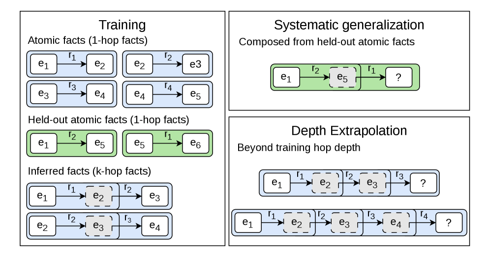## 3 Task Formulation We formally define our implicit reasoning setup using a synthetic multi-hop reasoning task, and categorize three generalization challenges under this formulation: in-distribution generalization, systematic generalization, and depth extrapolation (Figure 2). The latter two can be viewed as out-of-distribution (OOD) generalization. Such tasks have been shown to be difficult for vanilla transformers to learn (Yao et al., 2025), highlighting their limitations in composing parametric knowledge for reasoning (Allen-Zhu and Li, 2023; Yang et al., 2024b). ### 3.1 Task Definition <details> <summary>2604.07822v1/x2.png Details</summary>  ### Visual Description ## Diagram: Knowledge Graph Training and Generalization Framework ### Overview The diagram illustrates a framework for training and evaluating knowledge graphs, focusing on atomic facts, held-out facts, inferred facts, systematic generalization, and depth extrapolation. It uses colored boxes (blue, green) and arrows to represent relationships between entities (e1, e2, etc.) and relations (r1, r2, etc.). ### Components/Axes 1. **Training Section**: - **Atomic facts (1-hop facts)**: - Examples: `e1 →r1→ e2`, `e2 →r2→ e3`, `e3 →r3→ e4`, `e4 →r4→ e5` - **Held-out atomic facts (1-hop facts)**: - Examples: `e1 →r2→ e5`, `e5 →r1→ e6` (highlighted in green) - **Inferred facts (k-hop facts)**: - Examples: `e1 →r1→ e2 →r2→ e3`, `e2 →r2→ e3 →r3→ e4` (dashed arrows indicate inferred steps) 2. **Systematic Generalization**: - Composed from held-out atomic facts: `e1 →r2→ e5 →r1→ ?` (green boxes with a question mark for extrapolation) 3. **Depth Extrapolation**: - Beyond training hop depth: - Example 1: `e1 →r1→ e2 →r2→ e3 →r3→ ?` (3-hop sequence) - Example 2: `e1 →r1→ e2 →r2→ e3 →r3→ e4 →r4→ ?` (4-hop sequence) ### Detailed Analysis - **Training Section**: - Atomic facts represent direct, single-hop relationships (e.g., `e1 →r1→ e2`). - Held-out atomic facts are reserved for testing generalization (e.g., `e1 →r2→ e5`). - Inferred facts demonstrate multi-hop reasoning (e.g., `e1 →r1→ e2 →r2→ e3`). - **Systematic Generalization**: - Combines held-out facts to test if the model can generalize to unseen combinations (e.g., `e1 →r2→ e5 →r1→ ?`). - **Depth Extrapolation**: - Tests the model's ability to reason beyond the maximum hop depth seen during training (e.g., 3-hop or 4-hop sequences ending in `?`). ### Key Observations 1. **Color Coding**: - Blue boxes: Training data (atomic and inferred facts). - Green boxes: Held-out facts (systematic generalization). - Question marks (`?`): Unseen entities or relations for extrapolation. 2. **Flow Direction**: - Arrows (`→`) indicate directional relationships between entities. - Dashed arrows in inferred facts suggest multi-step reasoning. 3. **Progression**: - Training → Held-out → Inferred → Systematic Generalization → Depth Extrapolation shows increasing complexity. ### Interpretation This diagram demonstrates how knowledge graph models learn from structured data (atomic facts) and generalize to unseen combinations (systematic generalization) and longer reasoning chains (depth extrapolation). The use of held-out facts ensures the model isn't overfitting to training data, while depth extrapolation evaluates its capacity to handle multi-hop reasoning beyond explicit training examples. The progression from simple 1-hop facts to complex k-hop inferences highlights the model's ability to build and apply logical rules, a critical aspect of symbolic AI and graph neural networks. </details> Figure 2: Illustration of systematic and extrapolation generalization tasks with a sample dataset. Our implicit reasoning task relies on a directed knowledge graph (KG) where nodes represent a set of entities $E=\{e_i\}$ and edges represent a set of relations $R=\{r_j\}$ . The KG is composed of atomic (1-hop) facts, each taking the form of a triplet $(h,r,t)$ , where $h,t∈ E$ and $r∈ R$ (here $h$ and $t$ imply the head and tail entities, respectively). A $k$ -hop inferred fact is defined as a chain of $k$ atomic facts connecting a head entity $h$ to a final tail entity $t$ via a sequence of $k-1$ intermediate entities ( $i_1,\dots,i_k-1$ ): $$ (h,r_1,i_1),(i_1,r_2,i_2),\dots,(i_k-1,r_k,t) $$ Given the head entity $h$ and the sequence of relations $r_1,\dots,r_k$ , we use an auto-regressive decoder-only model to predict the final tail entity $t$ . The input prefix is $<e_h><r_1><r_2>\dots<r_k>$ , and the target is $<e_t>$ . Ideally, the model must implicitly perform the $k$ -hop traversal, successively retrieving each intermediate entity ( $i_1,\dots,i_k-1$ ) until it can resolve the final tail entity $t$ . ### 3.2 Generalization Challenges Given a generated knowledge graph, we first define the complete atomic fact set as $C=\{(h,r,t)\}$ , and the induced set of $k$ -hop inferred facts from $C$ as $$ I_k(C)=\{(h,r_1,\dots,r_k,t) \mid ∃ i_1,\dots,i_k-1, (h,r_1,i_1),\dots,(i_k-1,r_k,t)∈C\}. $$ #### Training set. The training set includes two parts: all possible atomic facts $C$ together with a set of inferred facts $I_train$ up to a maximum depth $k_train$ (e.g. $k$ -hop facts with $k∈[2,k_train]$ ). To characterize different generalization challenges, we partition the atomic fact set into two disjoint subsets $C=C_ID∪C_OOD$ . The training inferred facts $I_train$ can then be defined as $$ I_train=\{(h,r_1,\dots,r_k,t) \mid (h,r_1,\dots,r_k,t)∈I_k(C_ID), k≤ k_train\}. $$ We then define three generalization challenges: #### In-distribution generalization. The model is evaluated on inferred facts $(h,r_1,\dots,r_k,t)∈I_k(C_ID)$ that are not observed during training, equivalent to randomly sample inferred facts from $I_k(C_ID)$ as held-out test set. Despite its simplicity, previous work shows that vanilla transformers can only learn such tasks through extended training (Wang et al., 2024a). #### Systematic generalization. The model is evaluated on inferred facts $(h,r_1,\dots,r_k,t)∈I_k(C_OOD)$ , which are induced from atomic facts that are never used in compositions in the training data. This requires the learner to systematically combine its learned knowledge, without having seen combinations of it in training. This setting simulates scenarios where knowledge appears only as plain text in pretraining data (e.g. long-tail knowledge), but never forms answers to reasoning queries during training. Previous work (Wang et al., 2024a) shows that vanilla transformers completely fail on this generalization challenge. #### Depth extrapolation. The model is evaluated on inferred facts of greater depth than those included in the training dataset, i.e., $(h,r_1,\dots,r_k,t)∈I_k(C_ID)$ with $k$ larger than $k_train$ . Solving this requires the learner to infer the underlying rules of the task and iteratively apply them at depths far beyond those observed during training. This setting simulates scenarios where the complexity (i.e. reasoning depth) of training data is limited due to budget constraints, yet we expect the model to generalize beyond training. Such depth generalization poses challenges for vanilla transformers in symbolic (Kim and Linzen, 2020) and knowledge reasoning (Yao et al., 2025). Although related to length generalization, depth extrapolation is conceptually distinct: it measures the depth to which a model can repeatedly apply learned rules over its parametric knowledge beyond training. ## 4 Recurrent-Depth Transformer #### Model architecture. Across all experiments we use a decoder-only transformer with a recurrent-depth design illustrated in Figure 1. Concretely, we instantiate a GPT-2 style block with $L$ layers and reuse this for $R$ recurrent iterations, yielding an effective rolled-out depth of $D=L× R$ layers. At each recurrent iteration the same stack of layers is applied to the current hidden states. This allows the model to allocate more computation (increasing $R$ ) at inference time without changing the architecture or re-training the parameters. We exploit this property in our inference-time scaling experiments described in Section 6. Formally, let $f_θ$ denote the $L$ transformer layers with shared parameters $θ$ , and let $h^(0)$ be the input sequence after the initial embedding layer. The model computes $$ h^(r+1)=f_θ\big(h^(r);m\big), r=0,\dots,R-1, $$ where $m$ denotes the causal attention and padding masks. The final representation $h^(R)$ is passed through a final layer normalization and a tied output projection to produce logits over the vocabulary at each position. We only supervise the next-token distribution at the final position corresponding to the tail entity $t$ . Each entity and relation is represented by a dedicated token ( $<e_i>$ , $<r_j>$ ), and the query prefix is mapped to token embeddings. We adopt a zero-initialization strategy to stabilize training under repeated application of shared weights. Specifically, we initialize the output projection matrices (c_proj) of both the multi-head attention and feed-forward blocks to zero, so that each recurrent block is an exact identity mapping at initialization. This ensures that the input-output Jacobian remains stable even when the model is unrolled to a large number of recurrent iterations. This design is motivated by the known instability of deep networks with shared parameters (Agarwala and Schoenholz, 2022), which becomes particularly pronounced in recurrent-depth transformers (Saunshi et al., 2025). Following Zhang et al. (2019), this initialization supports stable optimization under unbounded unrolling of the recurrent iterations. #### Stopping strategies of the recurrent iterations. Training the looped transformer requires a stopping strategy to determine the number of recurrent iterations in the forward pass on the input. We consider two stopping strategies: fixed iteration and dynamic iteration. Fixed iteration determines the recurrent iterations to be the same fixed value for all training instances. The dynamic iteration strategy samples the number of recurrent iterations independently for each training batch. Concretely, for the dynamic model we sample $$ R∼clip\big(Poisson(λ),R_\min,R_\max\big), $$ where $R_\min$ and $R_\max$ are hyperparameters. Such strategies have been shown to be effective in realistic pretraining (Geiping et al., 2025; Zhu et al., 2025), and here we adopt a simple Poisson distribution to control the sampling distribution. Importantly, our strategies contrast with prior studies on the generalization ability of looped transformers, where the iteration number is matched to the complexity of each training instance, assuming oracle access to such complexity. Instead, our setup reflects practical scenarios (Geiping et al., 2025), where the complexity is unknown and computation cannot be allocated precisely in advance. ## 5 Systematic Generalization In this section, we study systematic generalization, i.e. whether models can combine parametric knowledge not composed during training for multi-hop tasks. We focus on $2$ -hop, as Wang et al. (2024a) shows that vanilla transformers already struggle with this simple task. ### 5.1 Experiment Setup #### Dataset. We construct the dataset by instantiating a knowledge graph with $|E|=2000$ and $|R|=200$ , where each entity has average out-degree 20. We then include all 40k atomic facts, randomly partitioned with 95% $C_ID$ , and 5% $C_OOD$ , together with 273.6k inferred facts for training. Our in-distribution set includes 3k held-out two-hop inferred facts composed from $C_ID$ , and OOD set includes nearly 2k two-hop inferred facts composed from $C_OOD$ . #### Model. We train our looped transformer with $L=4$ layers, and use fixed training recurrence with $R∈\{1,2,4,8\}$ . The model with $R=1$ is equivalent to a 4-layer vanilla transformer. We evaluate the accuracy of the predicted token against the gold answer. Absolute position embeddings (APE) (Vaswani et al., 2017) are used as positional embeddings in this setup. We do not use dynamic recurrence in this setting, as systematic generalization in the 2-hop task already emerges from weight sharing under fixed recurrence. In the multi-hop setting, however, it improves extrapolation to more complex samples at inference time and helps alleviate latent overthinking, as discussed in Section 6. ### 5.2 Results <details> <summary>2604.07822v1/x3.png Details</summary>  ### Visual Description ## Line Graphs: Model Performance Across Training Parameters ### Overview The image contains three line graphs comparing model accuracy across different training parameters (R values) and stages. Each graph uses distinct axes and visualizations to highlight performance trends. --- ### Components/Axes 1. **Left Graph** - **X-axis**: Epochs (0–8000) - **Y-axis**: Accuracy (0.00–1.00) - **Legend**: - R=1 (blue) - R=2 (orange) - R=4 (green) - R=8 (red) - **Shading**: Confidence intervals (light gray around lines). 2. **Middle Graph** - **X-axis**: Training Time (Hours) (0–40) - **Y-axis**: Accuracy (0.00–1.00) - **Legend**: Same R values as left graph. - **Shading**: Confidence intervals. 3. **Right Graph** - **X-axis**: Epochs (log scale, 10⁰–10⁴) - **Y-axis**: Accuracy (0.00–1.00) - **Legend**: - Train (blue) - Test ID (orange) - Test OOD (green) - **Vertical Dashed Lines**: Stage1, Stage2, Stage3 markers. --- ### Detailed Analysis #### Left Graph (Epochs vs Accuracy) - **R=1 (blue)**: Starts at ~0.05 accuracy, plateaus at ~0.75 by 2000 epochs. - **R=2 (orange)**: Gradual rise to ~0.75 by 6000 epochs. - **R=4 (green)**: Stable at ~0.75 from ~2000 epochs. - **R=8 (red)**: Sharp increase to ~0.85 by 6000 epochs. - **Uncertainty**: All lines have ±0.05–0.10 variability (shaded regions). #### Middle Graph (Training Time vs Accuracy) - **R=1 (blue)**: Reaches ~0.75 by 10 hours, then plateaus. - **R=2 (orange)**: Slower rise to ~0.75 by 30 hours. - **R=4 (green)**: Stable at ~0.75 after 10 hours. - **R=8 (red)**: Rapid rise to ~0.85 by 20 hours. #### Right Graph (Log-Scaled Epochs vs Accuracy) - **Train (blue)**: Exponential growth, plateaus at ~0.95 by 10³ epochs. - **Test ID (orange)**: Sharp rise to ~0.95 by 10² epochs, then plateaus. - **Test OOD (green)**: Gradual rise to ~0.75 by 10³ epochs. - **Stages**: - Stage1: ~10¹ epochs (blue/orange divergence). - Stage2: ~10² epochs (orange plateau). - Stage3: ~10³ epochs (green rise). --- ### Key Observations 1. **R Value Impact**: - Higher R (e.g., R=8) achieves faster convergence but risks overfitting (Test OOD lags Test ID). - Lower R (e.g., R=1) stabilizes earlier but with lower peak accuracy. 2. **Training Dynamics**: - Test OOD accuracy (~0.75) is significantly lower than Test ID (~0.95), suggesting poor generalization. - Log-scale visualization emphasizes early-stage performance differences. 3. **Stage Progression**: - Stage1: Initial training phase (blue/orange divergence). - Stage2: Model stabilization (orange plateau). - Stage3: OOD performance improvement (green rise). --- ### Interpretation - **Model Complexity Trade-off**: Higher R values improve training accuracy but may overfit, as seen in the disparity between Test ID and Test OOD. - **Efficiency vs Robustness**: Lower R values (e.g., R=1) train faster but sacrifice peak performance. - **Stage3 Significance**: The gradual rise in Test OOD accuracy suggests late-stage adaptation to out-of-distribution data, possibly through regularization or architectural adjustments. This analysis underscores the need to balance model complexity (R) with generalization goals, particularly for real-world deployment where OOD performance is critical. 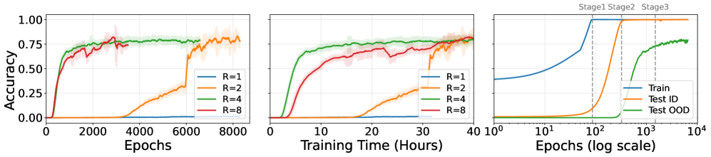</details> Figure 3: Accuracy curves for recurrent-depth models across training epochs and wall-clock time. Left: Test OOD accuracy for models trained with $R∈\{1,2,4,8\}$ , plotted against training epochs. Curves are smoothed with a 100-epoch rolling mean, with shading indicating standard deviation. Middle: Test OOD accuracy for the same models, plotted against training wall-clock time (hours). Right: Accuracy of the $R=4$ model on the examples from training, ID, and OOD test splits, plotted against training epochs. #### Recurrent-depth transformers perform systematic generalization, while vanilla transformers do not. On the left of Figure 3, we plot OOD accuracy as a function of training epochs. We find that the vanilla transformer (i.e. $R=1$ ) completely fails when the task requires combining unfamiliar atomic facts, while even the simplest $R=2$ recurrence achieves non-trivial generalization performance. Increasing training iterations further accelerates the convergence, e.g. $R=4$ converges with 2k epoch, while $R=2$ takes 7k. This acceleration is not only in terms of training steps, but also in absolute wall-clock time (Figure 3, middle). #### Systematic generalization emerges through a three-stage grokking dynamic. We further analyze the training dynamics of the $R=4$ model (right panel of Figure 3) to understand how systematic generalization emerges. We observe a three-stage dynamic: In the first stage, the model overfits the training set, with only training accuracy improving. In the second stage, in-distribution generalization emerges after prolonged training beyond memorization, a phenomenon referred to as grokking. In the final stage, systematic generalization arises only after the model achieves near-perfect in-distribution accuracy, occurring at a much later point than training overfitting (e.g., $10^4$ vs. $10^2$ epochs). #### Analyzing model internals with logit lens. 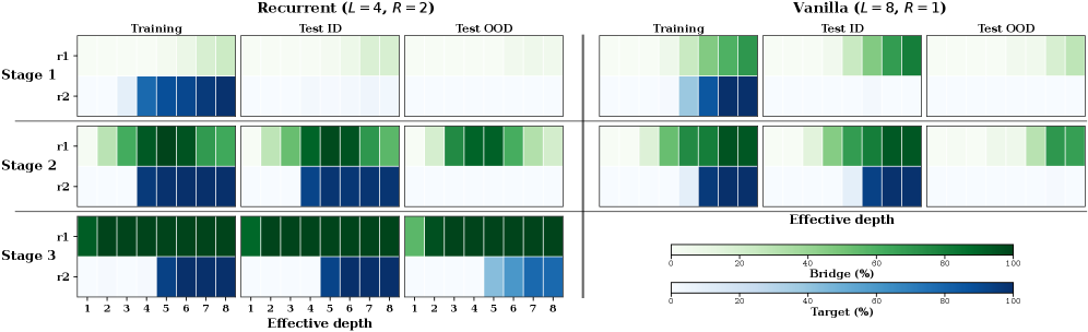We use the logit lens technique (nostalgebraist, 2020) to examine how models represent the bridge entity and the final target during different stages of training. After each layer and recurrent iteration, we project the intermediate hidden states through the final layer norm and language modeling head to obtain logits over the output vocabulary. For 2-hop inputs of the form $(h,r_1,r_2)$ , where $h$ is the head entity and $r_1,r_2$ are the two relations, we measure at each effective depth the accuracy of predicting the bridge entity at the $r_1$ position and the target entity at the $r_2$ position. Figure 4 shows logits lens for an $R=2$ recurrent-depth model on Training, Test ID, and Test OOD splits, across checkpoints corresponding to the three training stages. We compare against an iso-FLOP 8-layer vanilla transformer with matched effective depth. The vanilla model exhibits only two training stages and fails to achieve non-zero systematic generalization regardless of training time, consistent with Wang et al. (2024a). <details> <summary>2604.07822v1/x4.png Details</summary>  ### Visual Description ## Heatmap: Model Performance Across Stages and Effective Depth ### Overview The image presents a comparative heatmap analysis of two neural network architectures (Recurrent and Vanilla) across three stages (Stage 1-3) and eight effective depth levels (1-8). Performance metrics are visualized through color gradients representing "Bridge (%)" and "Target (%)" values, with separate panels for Training, Test ID, and Test OOD conditions. ### Components/Axes - **X-axis**: Effective depth (1-8) - **Y-axis**: - Recurrent model: Stage 1 (r1/r2), Stage 2 (r1/r2), Stage 3 (r1/r2) - Vanilla model: Stage 1, Stage 2, Stage 3 - **Legend**: - Bridge (%) (green gradient: 0-100%) - Target (%) (blue gradient: 0-100%) - **Panels**: - Left: Recurrent (L=4, R=2) - Right: Vanilla (L=8, R=1) - **Conditions**: Training, Test ID, Test OOD (horizontal grouping) ### Detailed Analysis #### Recurrent Model (L=4, R=2) - **Training**: - Stage 1: r1 shows 80-90% Bridge (dark green) at depths 1-3, dropping to 40-50% (light green) at depths 4-8. r2 shows 60-70% Bridge (medium green) at depths 1-4, declining to 20-30% (light green) at depths 5-8. - Stage 2: r1 maintains 70-80% Bridge (dark green) at depths 1-4, dropping to 30-40% (light green) at depths 5-8. r2 shows 50-60% Bridge (medium green) at depths 1-5, declining to 10-20% (light green) at depths 6-8. - Stage 3: r1 exhibits 60-70% Bridge (medium green) at depths 1-5, dropping to 10-20% (light green) at depths 6-8. r2 shows 40-50% Bridge (medium green) at depths 1-6, declining to 5-10% (light green) at depths 7-8. - **Test ID**: - Similar patterns to Training, with slightly higher Bridge percentages in early depths (e.g., Stage 1 r1: 85-95% Bridge at depths 1-3). - **Test OOD**: - Bridge percentages drop significantly: Stage 1 r1 shows 50-60% (medium green) at depths 1-3, declining to 10-20% (light green) at depths 4-8. r2 follows a similar trend but with shallower declines. #### Vanilla Model (L=8, R=1) - **Training**: - Stage 1: Bridge starts at 90% (dark green) at depth 1, dropping to 50% (medium green) at depth 4, then to 20% (light green) at depths 5-8. - Stage 2: Bridge declines from 80% (dark green) at depth 1 to 30% (light green) at depths 5-8. - Stage 3: Bridge drops from 70% (medium green) at depth 1 to 10% (light green) at depths 4-8. - **Test ID**: - Bridge percentages mirror Training but with slightly higher retention in early depths (e.g., Stage 1: 95% at depth 1, 60% at depth 4). - **Test OOD**: - Bridge percentages decline sharply: Stage 1 drops from 70% (medium green) at depth 1 to 10% (light green) at depths 3-8. Stage 3 shows near-zero Bridge (white) at depths 2-8. ### Key Observations 1. **Recurrent Advantage**: The Recurrent model consistently maintains higher Bridge percentages across all stages and depths compared to the Vanilla model, particularly in Test OOD conditions. 2. **Depth Sensitivity**: Both models show performance degradation with increasing effective depth, but the Recurrent model's decline is more gradual. 3. **Target vs. Bridge**: Target percentages (blue) generally follow inverse patterns to Bridge, with higher values in later depths for the Recurrent model. 4. **Stage Progression**: Performance deteriorates across stages for both models, with Stage 3 showing the most significant drops. ### Interpretation The data suggests that the Recurrent architecture (L=4, R=2) demonstrates superior robustness to varying effective depths and out-of-distribution (OOD) conditions compared to the Vanilla model (L=8, R=1). The Recurrent model's multi-stage design with recurrent connections (R=2) appears to better preserve learned representations across depths, maintaining higher Bridge percentages (shared knowledge transfer) even in challenging OOD scenarios. The Vanilla model's single-stage structure (R=1) with greater depth (L=8) suffers from more severe performance degradation, particularly in later stages and deeper layers. This aligns with the hypothesis that recurrent architectures with shallower depth but recurrent connections may be more effective for tasks requiring cross-depth knowledge integration. </details> Figure 4: Accuracy of predicting bridge and target entities using logit lens at corresponding token positions for the recurrent-depth ( $R=2$ ) and the 8-layer vanilla transformer. #### Grokking marks a transition from memorization to systematic generalization. We first focus on the recurrent-depth model (Figure 4 left panels), which exhibits distinct mechanisms across the three stages. In Stage 1, the model predicts targets without reliably decoding the bridge, indicating memorization. In Stage 2, the bridge becomes decodable, followed by correct target prediction for in-distribution data at deeper effective depths. Only in Stage 3 does the model succeed on OOD inputs, marking a transition from rote learning to systematic composition. In contrast, although vanilla transformers (right panels) can recover the bridge entity on Test OOD inputs, they fail to perform the second-hop reasoning, as they lack incentives to encode OOD facts in deeper layers. ## 6 Depth Extrapolation In this section, we study depth extrapolation, i.e., whether the model can perform deeper recursions when combining its parametric knowledge than those observed during training. <details> <summary>2604.07822v1/x5.png Details</summary>  ### Visual Description ## Heatmap: Recurrence vs. Hops Across Different R Values ### Overview The image is a composite heatmap visualization comparing recurrence patterns across multiple panels, each representing different model configurations (R=1 to R=8 and dynamic R). The visualization tracks recurrence values (r) against hop counts (k) with color intensity indicating magnitude. Key elements include: - Vertical dashed green lines marking ID/OOD boundaries - Horizontal purple lines indicating train recurrence thresholds - Color gradient from blue (low recurrence) to red (high recurrence) ### Components/Axes **Axes:** - **Y-axis (Recurrence, r):** Integer values 1-12 (logarithmic scale) - **X-axis (Hops, k):** Integer values 2-23 (linear scale) - **Legend:** - Green dashed line: ID/OOD boundary - Purple line: Train recurrence threshold - Color scale: Blue (0.00) to Red (1.00) **Panel Structure:** - 9 panels arranged in 3x3 grid - Panel titles specify R values and ID hop counts: - Top row: R=1 (2-hop), R=2 (6-hop), R=3 (9-hop) - Middle row: R=4 (10-hop), R=5 (12-hop), R=6 (13-hop) - Bottom row: R=7 (16-hop), R=8 (16-hop), R=dynamic (22-hop) ### Detailed Analysis **Color Distribution Patterns:** 1. **ID/OOD Boundary (Green Line):** - Position shifts rightward as R increases - R=1: k=11 | R=2: k=11 | R=3: k=11 | R=4: k=11 - R=5: k=14 | R=6: k=14 | R=7: k=17 | R=8: k=17 - Dynamic R: k=17 2. **Train Recurrence (Purple Line):** - Consistently at r=8 across all panels - Exception: R=1 panel shows no visible purple line 3. **Recurrence Intensity:** - Blue dominance (low recurrence) in upper-right regions - Red dominance (high recurrence) in lower-left regions - Gradual transition from blue to red as R increases **Notable Data Points:** - R=1 panel: Entirely blue except for k=2-5 (partial red) - R=8 panel: Strong red region at k=2-10, r=5-8 - Dynamic R panel: Most extensive red region (k=2-17, r=5-12) ### Key Observations 1. **Boundary Shift:** ID/OOD boundary moves rightward with increasing R (k=11→17) 2. **Recurrence Concentration:** Higher R values show stronger recurrence in lower hop ranges 3. **Train Recurrence Consistency:** Purple line remains at r=8 across all configurations 4. **Dynamic R Anomaly:** Largest hop range (2-358) with most pronounced red region ### Interpretation The visualization demonstrates that: 1. **Model Complexity Impact:** Increasing R values correlate with rightward shifts in ID/OOD boundaries, suggesting greater model capacity to distinguish in-distribution data 2. **Recurrence Thresholding:** The consistent r=8 threshold across configurations may represent an optimal performance benchmark 3. **Hop-Recurrence Relationship:** Lower hop counts (k=2-10) consistently show higher recurrence values, indicating stronger pattern recognition in early stages 4. **Dynamic R Behavior:** The extended hop range (up to 358) with concentrated red region suggests specialized handling of longer sequences The color gradient intensity and boundary positioning imply that model configuration (R value) significantly influences both data separation capabilities and recurrence pattern recognition. The dynamic R configuration appears optimized for handling extended sequence lengths while maintaining strong recurrence in early hops. 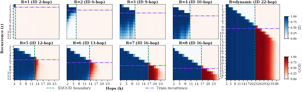</details> Figure 5: Accuracy of recurrent-depth models on multi-hop composition, trained under various fixed and dynamic recurrence setups. The violet dash-dotted horizontal line indicates the training recurrence (or maximum in the dynamic setting), while the teal dashed vertical line marks the maximum ID generalization achieved by each model. The x-axis shows hop complexity and the y-axis shows inference-time recurrence ( $r^*$ denotes adaptive halting). ### 6.1 Experiment Setup #### Curriculum training. Different from 2-hop scenarios, learning $k$ -hop tasks generally requires training the model with an easy-to-hard curriculum over hop depth ( $k$ ) as suggested in Yao et al. (2025). Specifically, we start with training on atomic and 2-hop facts until an accuracy threshold ( $95\$ ) is reached on a held-out 2-hop test split. Next, 3-hop data is included in the training for the next stage of our curriculum until $95\$ is achieved on the held-out 3-hop test split. This process is repeated for each hop level $k∈\{2,\dots,N_\max\}$ . To prevent forgetting, at each stage we jointly train on all previously introduced facts (e.g., at stage $k=5$ we train on atomic and 2-hop through 5-hop facts). Due to this threshold-based curriculum, training facts beyond the model’s capability are never exposed. That is, if the model fails to achieve above-threshold accuracy on $k$ -hop queries, training terminates and $(k+1)$ -hop data is never introduced. We define the largest such $k$ as the learnable recursion depth of the model. #### Dataset. We construct the dataset by instantiating a knowledge graph with $|E|=200$ entities and $|R|=10$ relations, where each entity has an average out-degree of 10. We additionally impose a permutation constraint on the knowledge graph to avoid learning shortcut solutions, for which we provide details in Appendix B. We pre-generate 2k atomic facts and 15k $k$ -hop inferred facts for each $k∈[2,K_max]$ , with $K_max=40$ . During training, these facts are progressively introduced following the curriculum described above. For each model, we evaluate on 750 held-out $k$ -hop facts. Facts with $k$ up to the model’s learnable recursion depth form the in-distribution test set, while those beyond it constitute the extrapolation test set. This split is model-dependent, reflecting each model’s maximum achievable reasoning depth. #### Model. We follow the model setups in Section 5.1, except that we use $R∈$ {1,2,3,4,5,6,7,8} for fixed iteration. Here we use no positional embeddings (NoPE) (Kazemnejad et al., 2023; Wang et al., 2024b), which shows better generalization in pilot studies. In addition to results with $L=4$ , we present results with varying model size and dynamic train recurrence in Appendix F, and across random seed initializations in Appendix G. ### 6.2 In-Distribution Generalization #### Scaling up training-time iteration increases the learnable recursion depth of looped transformers. Looking at the blue area of Figure 5, we find that increasing training recurrent iterations accordingly improves the ID generalization. This is consistent with previous findings (Wang et al., 2024a; Yao et al., 2025) that the learnable recursion depth of a transformer is bounded by the depth of its layers, and we demonstrate that for looped transformers, scaling up training recurrent iterations can also increase its ”effective depth”, without relying on additional parameters. Training with dynamic iteration further increases the learnable recursion depth over the fixed iteration, suggesting that the fixed iteration is not an optimal design choice. Interestingly, more recurrent iterations do not always translate into larger learnable depth. (e.g., both R=7 and R=8 learns up to 16-hop task). <details> <summary>2604.07822v1/x6.png Details</summary>  ### Visual Description ## Line Graph: Update Steps vs ID Hops Generalized (k) ### Overview The graph illustrates the relationship between "Update Steps" (y-axis) and "ID Hops Generalized (k)" (x-axis). The y-axis uses a logarithmic scale (1e6), and the x-axis ranges from 2 to 22. A single blue line represents the data, with a notable plateau followed by a sharp increase. ### Components/Axes - **Y-Axis**: Labeled "Update Steps" with a logarithmic scale (1e6). Tick marks at 0.5, 1.0, 1.5, and 2.0 (units: 1e6). - **X-Axis**: Labeled "ID Hops Generalized (k)" with integer markers from 2 to 22. - **Legend**: Located in the top-right corner, indicating "Update Steps" with a blue line. - **Line**: Blue, single data series, plotted with markers at each x-axis value. ### Detailed Analysis - **Initial Rise**: At k=2, the line starts at approximately 0.5e6 update steps. By k=4, it rises sharply to ~1.3e6 and remains flat until k=14. - **Plateau**: From k=4 to k=14, update steps stabilize at ~1.3e6. - **Post-Plateau Increase**: After k=14, the line gradually increases to ~1.5e6 by k=18, then accelerates sharply to ~2.0e6 at k=22. ### Key Observations 1. **Stability**: A prolonged plateau (k=4–14) suggests minimal update steps for moderate k values. 2. **Threshold Effect**: A sharp increase begins at k=18, indicating a potential system threshold or inefficiency at higher k values. 3. **Logarithmic Scale Impact**: The y-axis compression makes the final spike (k=18–22) appear steeper than its absolute magnitude (0.5e6 increase). ### Interpretation The data implies that update steps remain efficient for k ≤ 14 but degrade significantly as k approaches 22. This could reflect a computational bottleneck or algorithmic inefficiency at higher k values. The logarithmic y-axis may exaggerate the perceived severity of the final increase, warranting further investigation into the system's behavior beyond k=14. The plateau suggests an optimized range for k, while the post-plateau trend highlights a critical failure point requiring optimization. 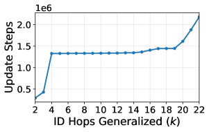</details> Figure 6: Cumulative gradient updates required to first generalize to each hop complexity. #### Phase transition from prolonged training to rapid learning. We observe that models require a prolonged training phase to acquire low-hop tasks, after which they rapidly generalize to much more complex samples (Figure 6). We illustrate this for the model trained with dynamic recurrence by plotting training steps against the compositional complexity achieved on in-distribution data. This suggests that the main difficulty lies in discovering the underlying compositional rule. Once such a rule is internalized, the model can quickly extend it to samples of much higher complexity. In Figure 6 we observe how the model required over 1.3 million steps for grokking up to 4-hop train samples but was quickly able to learn up to 19-hop samples very few additional steps. Beyond that, for even more complex samples, while each new hop requires additional training steps to cross the 95% threshold, the model still achieves strong generalization (>90%) on hops 20, 21, and 22 within fewer than 8k extra steps per hop which is commensurate with the steps required for each additional hop from 4 through 19. By loading a trained checkpoint (20, say) and continuing training exclusively on 21-hop samples instead of the data mix consisting of samples from all previous stages in our curriculum, generalization over 90% on the new split can be achieved in as little as 50 additional steps of training. ### 6.3 Depth Extrapolation #### Scaling inference-time iterations unlocks depth extrapolation. In Figure 5, we observe that when using the same number of recurrent iterations as in training, all models struggle to generalize to tasks of higher complexity than those seen during training. However, this limitation is immediately alleviated when we increase the number of inference-time iterations, with more iterations enabling generalization to progressively harder tasks. Notably, this scaling effect only emerges for $R>4$ , suggesting that sufficient training-time iterations are a prerequisite for benefiting from increased inference-time computation. #### The effect of training iteration strategy on extrapolation. 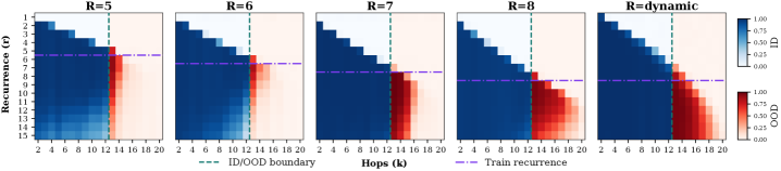The above results characterize the maximum reasoning depth each model can achieve under the curriculum setting, but they do not disentangle whether the differences (e.g. $R=6$ generalizing to $17$ -hop vs. $R=8$ to $24$ -hop) are due to more training iterations or exposure to more complex training data (e.g. $R=6$ is trained up to $13$ -hop, while $R=8$ up to $16$ -hop). To isolate the effect of the training iteration strategy, we train all models on the same data (up to $12$ -hop) and evaluate extrapolation on $12$ – $24$ hop tasks. <details> <summary>2604.07822v1/x7.png Details</summary>  ### Visual Description ## Heatmap: Model Performance Across R Values and Hops ### Overview The image displays a heatmap visualization comparing model performance across different recurrence values (R) and hop counts (k). It consists of five panels labeled R=5, R=6, R=7, R=8, and R=dynamic, showing the transition between in-distribution (ID) and out-of-distribution (OOD) data regions. ### Components/Axes - **X-axis (Hops)**: Labeled "Hops (k)" with values ranging from 2 to 20. - **Y-axis (Recurrence)**: Labeled "Recurrence (r)" with values from 2 to 15. - **Legend**: - Dashed green line: "ID/OOD boundary" - Purple dashed line: "Train recurrence" - Color scale: Blue (ID) to Red (OOD), with a gradient from 0.00 to 1.00. ### Detailed Analysis 1. **R=5 Panel**: - ID/OOD boundary (dashed line) at k≈12. - Train recurrence (purple line) at r=7. - ID region (blue) dominates left of the boundary; OOD (red) appears right of the boundary. 2. **R=6 Panel**: - ID/OOD boundary shifts right to k≈13. - Train recurrence remains at r=7. - OOD region expands slightly compared to R=5. 3. **R=7 Panel**: - ID/OOD boundary at k≈14. - Train recurrence still at r=7. - OOD region grows further, with red intensity increasing. 4. **R=8 Panel**: - ID/OOD boundary at k≈15. - Train recurrence unchanged at r=7. - OOD region dominates the right half of the panel. 5. **R=dynamic Panel**: - ID/OOD boundary at k≈16. - Train recurrence persists at r=7. - OOD region occupies the majority of the panel, with red intensity peaking. ### Key Observations - **Boundary Shift**: The ID/OOD boundary moves rightward as R increases, indicating a gradual shift in model behavior. - **Train Recurrence Consistency**: The purple line (r=7) remains fixed across all panels, suggesting a stable training parameter. - **OOD Expansion**: Higher R values correlate with larger OOD regions, implying reduced model robustness to out-of-distribution data as R increases. ### Interpretation The heatmap demonstrates that increasing R values shift the model's ID/OOD boundary toward higher hop counts, suggesting that the model's ability to distinguish in-distribution data degrades with higher R. The constant train recurrence (r=7) implies this parameter was fixed during training, while the dynamic R panel shows the most pronounced OOD dominance, highlighting potential instability in model performance under variable recurrence settings. The color gradient confirms that OOD regions (red) become more prevalent as R increases, indicating a critical trend for model evaluation under varying conditions. </details> Figure 7: Accuracy of models trained with fixed recurrence $R∈\{5,6,7,8\}$ and dynamic recurrence on up to 12-hop samples. From Figure 7, we first find that among fixed-iteration models, increasing the number of training-time iterations substantially improves extrapolation when scaling inference-time iterations (e.g. $R=6$ extrapolates up to $14$ -hop, while $R=8$ reaches $19$ -hop). Second, under the same training data, the dynamic iteration strategy achieves comparable extrapolation performance to the $R=8$ model (both reaching $19$ -hop). This contrasts with Figure 5, where the dynamic strategy generalizes to significantly higher complexity than $R=8$ . These results suggest that the maximum number of iterations used during training determines the extrapolation range (i.e. how far beyond the training complexity the model can generalize), while dynamic iteration effectively exploits this range, since it enables a larger learnable recursion depth. Hence, when training data is sufficiently complex, dynamic iteration should be preferred over fixed strategies with the same maximum iteration budget. #### Scaling inference-time iterations is limited by overthinking. Despite strong generalization performance, we observe performance degradation when using excessively large inference-time iterations. For example, increasing iterations beyond 15 for the R=dynamic does not improve OOD performance (Figure 5), a phenomenon known as overthinking (Bansal et al., 2022). We study this along two key axes: (1) inference iterations, i.e. how increasing the inference iterations affects the model’s prediction confidence, and (2) task complexity, i.e. how increasing task complexity impacts this confidence. <details> <summary>2604.07822v1/x8.png Details</summary>  ### Visual Description ## Line Graphs: Margin vs. Recurrent Iteration for Different R Values ### Overview The image contains four line graphs comparing the "Margin" metric across recurrent iterations (t) for different system configurations labeled R=6, R=7, R=8, and R=dynamic. Each graph includes multiple colored lines representing different "hop" configurations (2-hop, 5-hop, 10-hop, etc.), with a legend at the bottom. Vertical dashed lines mark "Avg. first-hit t*" thresholds, and a horizontal line at Margin=0 serves as a reference. ### Components/Axes - **X-axis**: Recurrent Iteration (t), ranging from 1 to 25. - **Y-axis**: Margin, with scales varying per graph (e.g., -25 to 50 for R=6, -10 to 20 for R=7, etc.). - **Legend**: Located at the bottom, mapping colors to hop configurations: - Blue: 2-hop - Orange: 5-hop - Green: 10-hop - Red: 13-hop - Purple: 16-hop - Brown: 30-hop - Dashed black line: Margin = 0 - Vertical dashed lines: Avg. first-hit t* (exact values vary per graph). ### Detailed Analysis #### R=6 Graph - **Y-axis range**: -25 to 50. - **Trends**: - All lines start near 0 and diverge sharply downward. - 2-hop (blue) drops steeply, crossing Margin=0 at t≈5. - Higher hops (e.g., 30-hop, brown) decline more gradually. - Vertical dashed lines (Avg. first-hit t*) appear near t=3–5. #### R=7 Graph - **Y-axis range**: -10 to 20. - **Trends**: - Lines start near 0 and decline, with 2-hop (blue) crossing Margin=0 at t≈4. - 30-hop (brown) remains above Margin=0 until t≈10. - Avg. first-hit t* marked near t=2–4. #### R=8 Graph - **Y-axis range**: -5 to 10. - **Trends**: - 2-hop (blue) crosses Margin=0 at t≈3. - 30-hop (brown) stays positive until t≈8. - Avg. first-hit t* marked near t=1–3. #### R=dynamic Graph - **Y-axis range**: 0 to 10. - **Trends**: - Lines converge sharply at t=10, with 30-hop (brown) dropping to Margin=0. - Avg. first-hit t* marked at t=10. ### Key Observations 1. **Margin Decline**: All configurations show a general decline in Margin with increasing t, but the rate varies by R and hop count. 2. **First-Hit Thresholds**: Avg. first-hit t* occurs earlier for lower R values (e.g., t≈3 for R=8) and later for higher R (e.g., t≈10 for R=dynamic). 3. **Hop Count Impact**: Lower-hop configurations (e.g., 2-hop) reach Margin=0 faster than higher-hop ones (e.g., 30-hop). 4. **Dynamic R Behavior**: The R=dynamic graph shows a sudden convergence at t=10, suggesting a threshold-based adjustment. ### Interpretation The data suggests that system performance (as measured by Margin) deteriorates with recurrent iterations, but the speed of decline depends on R and hop count. Lower R values and fewer hops lead to faster Margin collapse, while higher R or hop counts delay this effect. The "Avg. first-hit t*" thresholds likely represent critical points where system stability or efficiency thresholds are breached. The R=dynamic configuration’s abrupt change at t=10 implies a mechanism to reset or adjust parameters when Margin approaches zero, preventing further decline. This could indicate adaptive behavior in dynamic systems to maintain performance under varying conditions. 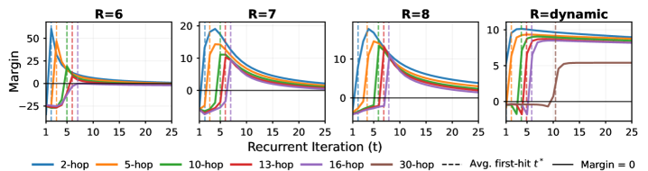</details> Figure 8: Average logit margin across recurrent iterations for fixed-recurrence ( $R=6,7,8$ ) and dynamic-recurrence models. Curves show different hop complexities, and dashed vertical lines indicate the average first-hit iteration $t^*$ (when the correct entity is predicted). In Figure 8, we analyze the logit margin, defined as the difference between the logit of the correct entity and that of the strongest competing token, and make two observations. First, across all models and tasks, the margin increases with inference iterations until reaching a peak, and then consistently declines as iterations continue. This suggests that overthinking arises as the iteration number grows, regardless of the task complexity. Notably, the dynamic model exhibits a much slower margin decay compared to fixed-iteration models, indicating that dynamic iteration is more robust to overthinking. Second, the peak margin decreases as task complexity increases across all models. This implies that for more complex tasks, the model’s predictions are inherently less confident and therefore more susceptible to degradation under additional iterations. As a result, the benefit of increasing inference iterations diminishes for highly complex tasks. Note that although previous work mitigates overthinking by injecting inputs information in every iteration (Bansal et al., 2022; Geiping et al., 2025), we find that such methods do not resolve the issue in implicit reasoning. <details> <summary>2604.07822v1/x9.png Details</summary>  ### Visual Description ## Line Graph: Average Iterations vs. Sample Complexity (k) ### Overview The image is a line graph comparing the performance of two methods ("Ours" and "KL-only") across varying sample complexities (k). The x-axis represents sample complexity (k), ranging from 2 to 37, while the y-axis represents average iterations, scaled from 0 to 15. Two data series are plotted: a blue line labeled "Ours" and an orange line labeled "KL-only". ### Components/Axes - **X-axis (Sample Complexity, k)**: - Labels: "Sample Complexity (k)". - Ticks: 2, 7, 12, 17, 22, 27, 32, 37. - Scale: Linear increments of 5. - **Y-axis (Average Iterations)**: - Labels: "Avg. Iterations". - Ticks: 0, 5, 10, 15. - Scale: Linear increments of 5. - **Legend**: - Position: Top-right corner. - Entries: - Blue line: "Ours". - Orange line: "KL-only". ### Detailed Analysis - **Blue Line ("Ours")**: - Starts at approximately (2, 2) and increases steadily. - At k=37, reaches ~15 iterations. - Slope: Consistent upward trend with no plateaus or declines. - **Orange Line ("KL-only")**: - Starts similarly to "Ours" but peaks at ~10 iterations around k=22. - Declines sharply after k=22, reaching ~4 iterations by k=37. - Notable inflection point: k=22 (peak) followed by a steep drop. ### Key Observations 1. **Divergence at k=22**: The "KL-only" method peaks at k=22 (~10 iterations) and then declines, while "Ours" continues to rise. 2. **Performance Gap**: By k=37, "Ours" achieves ~15 iterations, whereas "KL-only" drops to ~4 iterations. 3. **Initial Similarity**: Both methods start with nearly identical performance at low k values (e.g., k=2–7). ### Interpretation The data suggests that the "Ours" method scales more effectively with increasing sample complexity compared to "KL-only". The "KL-only" method exhibits a performance ceiling, peaking at moderate k values before degrading, potentially due to overfitting or inefficiency at higher complexities. In contrast, "Ours" maintains a linear improvement, indicating robustness or adaptive optimization. This divergence highlights a critical threshold (k≈22) where "KL-only" becomes less viable, while "Ours" remains consistently effective. The results imply that "Ours" may be preferable for high-complexity scenarios, whereas "KL-only" might suffice for simpler tasks but fails to generalize. 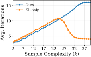</details> Figure 9: Average recurrent iterations using adaptive halting vs. sample complexity. #### Adaptive halting improves inference efficiency. 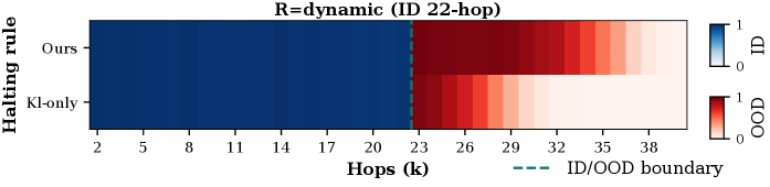We flexibly halt recurrence in order to allocate compute proportionate to input complexity. Prior work (Geiping et al., 2025) proposes adaptive halting based on the output distribution $p_t(·\mid x)$ , terminating when the change between successive iterations becomes small, measured by $KL\bigl(p_t,|,p_t-1\bigr)<ε_KL$ . In our setting, we find that this criterion often halts the recurrence prematurely, leading to suboptimal performance. To address this, we additionally incorporate the entropy of the output distribution, $H(p_t)$ , and only stop when both the divergence is small, and the prediction is confident, i.e., $$ KL\bigl(p_t \| p_t-1\bigr)<ε_KL and H(p_t)<H_thresh. $$ In Figure 9, we plot the number of iterations using both methods against the hop count ( $k$ ), demonstrating that ours results in better allocation of inference-time compute in accordance with task complexity. While the output distribution may change very little across iterations, the entropy is still high, indicating that the model remains uncertain despite this apparent convergence. We compare results using the two methods in Figure 10. In our setting, combining KL divergence with entropy therefore provides a more reliable halting signal and yields better overall results. <details> <summary>2604.07822v1/x10.png Details</summary>  ### Visual Description ## Heatmap: R=dynamic (ID 22-hop) Halting Rule Performance ### Overview This heatmap visualizes the performance of two halting rules ("Ours" and "Kl-only") across varying numbers of hops (k=2 to 38) in a dynamic R environment (ID 22-hop). A dashed vertical line at k=23 marks the ID/OOD boundary, with color gradients indicating performance scores (0=blue, 1=red). ### Components/Axes - **X-axis (Hops (k))**: Integer values from 2 to 38, representing the number of hops. - **Y-axis (Halting rule)**: Two categories: - "Ours" (dark blue) - "Kl-only" (red-to-white gradient) - **Legend**: - Blue (0) to Red (1) gradient, indicating performance scores. - Dashed line at k=23 labeled "ID/OOD boundary". ### Detailed Analysis - **"Ours" (dark blue)**: - Uniform dark blue across all hops (k=2–38), indicating a consistent performance score of **0**. - No variation observed, suggesting stable behavior across all hops. - **"Kl-only" (red-to-white gradient)**: - Starts as dark red (score ~1) at k=2–22. - Gradually transitions to light red (score ~0.5) at k=23–29. - Becomes white (score ~0) at k=30–38. - The transition aligns with the ID/OOD boundary at k=23. ### Key Observations 1. **"Ours" maintains a constant 0 score**, implying no performance degradation or improvement with increasing hops. 2. **"Kl-only" shows a clear decline** in performance (from 1 to 0) as hops increase, with a sharp transition at k=23. 3. The **ID/OOD boundary at k=23** coincides with the midpoint of the "Kl-only" gradient, suggesting a critical threshold for model behavior. ### Interpretation - **"Ours" demonstrates robustness**: Its consistent performance (score=0) across all hops suggests it is unaffected by the number of hops or the ID/OOD boundary. - **"Kl-only" exhibits sensitivity**: The gradient indicates performance degradation as hops increase, with a notable shift at k=23. This may reflect overfitting to in-distribution data (k<23) and failure to generalize beyond the boundary. - The **ID/OOD boundary at k=23** acts as a pivot point for "Kl-only", highlighting its reliance on hop count for performance. This contrasts with "Ours", which remains invariant, potentially due to architectural or algorithmic differences in handling dynamic R environments. </details> Figure 10: Comparison of adaptive halting based on KL-divergence and entropy (ours) versus KL-divergence alone (Geiping et al., 2025). ## 7 Conclusion We study whether recurrent-depth transformers can compositionally use parametric knowledge for implicit multi-hop reasoning, a task that is challenging for vanilla transformers. Through controlled experiments on models trained from scratch, we show that recurrent-depth transformers successfully address both compositional generalization challenges. Systematic generalization emerges through a three-stage grokking dynamic, as the model transitions from rote memorization to generalizable solutions. Depth extrapolation is enabled by scaling inference-time compute, where additional iterations allow for greater reasoning depth, although latent overthinking limits performance on highly complex tasks. Overall, our results highlight recurrent-depth transformers as a promising architecture for compositional reasoning over parametric knowledge. ## Acknowledgments The authors of this paper express their gratitude to Boshi Wang for valuable discussions on this work, and for motivating the permutation-based task formulation for depth exploration described in Appendix B. We also thank Yupei Du for valuable feedback on this paper. ## References - A. Agarwala and S. S. Schoenholz (2022) Deep equilibrium networks are sensitive to initialization statistics. In International Conference on Machine Learning, pp. 136–160. Cited by: §4. - Z. Allen-Zhu and Y. Li (2023) Physics of language models: part 3.1, knowledge storage and extraction. arXiv preprint arXiv:2309.14316. Cited by: §3. - M. Balesni, T. Korbak, and O. Evans (2024) The two-hop curse: llms trained on $A→ B$ , $B→ C$ fail to learn $A→ C$ . arXiv preprint arXiv:2411.16353. Cited by: Appendix D. - A. Bansal, A. Schwarzschild, E. Borgnia, Z. Emam, F. Huang, M. Goldblum, and T. Goldstein (2022) End-to-end algorithm synthesis with recurrent networks: extrapolation without overthinking. Advances in Neural Information Processing Systems 35, pp. 20232–20242. Cited by: §1, §1, §6.3, §6.3. - L. Berglund, M. Tong, M. Kaufmann, M. Balesni, A. C. Stickland, T. Korbak, and O. Evans (2023) The reversal curse: llms trained on” a is b” fail to learn” b is a”. arXiv preprint arXiv:2309.12288. Cited by: §1. - E. Biran, D. Gottesman, S. Yang, M. Geva, and A. Globerson (2024) Hopping too late: exploring the limitations of large language models on multi-hop queries. In Proceedings of the 2024 Conference on Empirical Methods in Natural Language Processing, Y. Al-Onaizan, M. Bansal, and Y. Chen (Eds.), Miami, Florida, USA, pp. 14113–14130. External Links: Link, Document Cited by: §1. - T. Brown, B. Mann, N. Ryder, M. Subbiah, J. D. Kaplan, P. Dhariwal, A. Neelakantan, P. Shyam, G. Sastry, A. Askell, et al. (2020) Language models are few-shot learners. Advances in neural information processing systems 33, pp. 1877–1901. Cited by: §1. - M. Dehghani, S. Gouws, O. Vinyals, J. Uszkoreit, and L. Kaiser (2019) Universal transformers. In International Conference on Learning Representations, External Links: Link Cited by: Appendix D, §1. - H. Du, Y. Dong, and X. Ning (2025) Latent thinking optimization: your latent reasoning language model secretly encodes reward signals in its latent thoughts. arXiv preprint arXiv:2509.26314. Cited by: Appendix D. - N. Dziri, X. Lu, M. Sclar, X. L. Li, L. Jiang, B. Y. Lin, P. West, C. Bhagavatula, R. Le Bras, J. D. Hwang, S. Sanyal, S. Welleck, X. Ren, A. Ettinger, Z. Harchaoui, and Y. Choi (2023) Faith and fate: limits of transformers on compositionality. In Proceedings of the 37th International Conference on Neural Information Processing Systems, NIPS ’23, Red Hook, NY, USA. Cited by: Appendix D, §1. - Y. Fan, Y. Du, K. Ramchandran, and K. Lee (2025) Looped transformers for length generalization. In The Thirteenth International Conference on Learning Representations, External Links: Link Cited by: §1, §2, §2. - L. Gao, S. Biderman, S. Black, L. Golding, T. Hoppe, C. Foster, J. Phang, H. He, A. Thite, N. Nabeshima, et al. (2020) The pile: an 800gb dataset of diverse text for language modeling. arXiv preprint arXiv:2101.00027. Cited by: §2. - J. Geiping, S. M. McLeish, N. Jain, J. Kirchenbauer, S. Singh, B. R. Bartoldson, B. Kailkhura, A. Bhatele, and T. Goldstein (2025) Scaling up test-time compute with latent reasoning: a recurrent depth approach. In ES-FoMo III: 3rd Workshop on Efficient Systems for Foundation Models, External Links: Link Cited by: Appendix D, §1, §4, Figure 10, §6.3, §6.3. - M. Geva, J. Bastings, K. Filippova, and A. Globerson (2023) Dissecting recall of factual associations in auto-regressive language models. In Proceedings of the 2023 Conference on Empirical Methods in Natural Language Processing, H. Bouamor, J. Pino, and K. Bali (Eds.), Singapore, pp. 12216–12235. External Links: Link, Document Cited by: §1. - S. Hao, S. Sukhbaatar, D. Su, X. Li, Z. Hu, J. E. Weston, and Y. Tian (2025) Training large language models to reason in a continuous latent space. In Second Conference on Language Modeling, External Links: Link Cited by: Appendix D. - J. Huang and K. C. Chang (2023) Towards reasoning in large language models: a survey. In Findings of the Association for Computational Linguistics, ACL 2023, pp. 1049–1065. Cited by: Appendix A. - A. Kazemnejad, I. Padhi, K. Natesan Ramamurthy, P. Das, and S. Reddy (2023) The impact of positional encoding on length generalization in transformers. Advances in Neural Information Processing Systems 36, pp. 24892–24928. Cited by: §6.1. - N. Kim and T. Linzen (2020) COGS: a compositional generalization challenge based on semantic interpretation. In Proceedings of the 2020 Conference on Empirical Methods in Natural Language Processing (EMNLP), B. Webber, T. Cohn, Y. He, and Y. Liu (Eds.), Online, pp. 9087–9105. External Links: Link, Document Cited by: §3.2. - H. Kohli, S. Kumar, and H. Sun (2025) GroundCocoa: a benchmark for evaluating compositional & conditional reasoning in language models. In Proceedings of the 2025 Conference of the Nations of the Americas Chapter of the Association for Computational Linguistics: Human Language Technologies (Volume 1: Long Papers), L. Chiruzzo, A. Ritter, and L. Wang (Eds.), Albuquerque, New Mexico, pp. 8280–8295. External Links: Link, Document, ISBN 979-8-89176-189-6 Cited by: Appendix D. - B. Lake and M. Baroni (2018) Generalization without systematicity: on the compositional skills of sequence-to-sequence recurrent networks. In International conference on machine learning, pp. 2873–2882. Cited by: §1. - Z. Lan, M. Chen, S. Goodman, K. Gimpel, P. Sharma, and R. Soricut (2020) ALBERT: a lite bert for self-supervised learning of language representations. In International Conference on Learning Representations, External Links: Link Cited by: Appendix D. - [22] I. Loshchilov and F. Hutter Decoupled weight decay regularization. In International Conference on Learning Representations, Cited by: Appendix C. - W. Lu, Y. Yang, K. Lee, Y. Li, and E. Liu (2025) Latent chain-of-thought? decoding the depth-recurrent transformer. arXiv preprint arXiv:2507.02199. Cited by: Appendix D. - nostalgebraist (2020) Interpreting gpt: the logit lens. External Links: Link Cited by: §5.2. - O. Press, M. Zhang, S. Min, L. Schmidt, N. Smith, and M. Lewis (2023) Measuring and narrowing the compositionality gap in language models. In Findings of the Association for Computational Linguistics: EMNLP 2023, H. Bouamor, J. Pino, and K. Bali (Eds.), Singapore, pp. 5687–5711. External Links: Link, Document Cited by: §1. - N. Saunshi, N. Dikkala, Z. Li, S. Kumar, and S. J. Reddi (2025) Reasoning with latent thoughts: on the power of looped transformers. In The Thirteenth International Conference on Learning Representations, External Links: Link Cited by: Figure 1, §2, §4. - H. A. Simon and A. Newell (1971) Human problem solving: the state of the theory in 1970.. American Psychologist 26, pp. 145–159. External Links: Link Cited by: Appendix D. - A. Vaswani, N. Shazeer, N. Parmar, J. Uszkoreit, L. Jones, A. N. Gomez, Ł. Kaiser, and I. Polosukhin (2017) Attention is all you need. In Advances in Neural Information Processing Systems, I. Guyon, U. V. Luxburg, S. Bengio, H. Wallach, R. Fergus, S. Vishwanathan, and R. Garnett (Eds.), Vol. 30, pp. . External Links: Link Cited by: §5.1. - B. Wang, X. Yue, Y. Su, and H. Sun (2024a) Grokking of implicit reasoning in transformers: a mechanistic journey to the edge of generalization. In Proceedings of the 38th International Conference on Neural Information Processing Systems, NIPS ’24, Red Hook, NY, USA. External Links: ISBN 9798331314385 Cited by: Appendix D, §1, §3.2, §3.2, §5.2, §5, §6.2. - J. Wang, T. Ji, Y. Wu, H. Yan, T. Gui, Q. Zhang, X. Huang, and X. Wang (2024b) Length generalization of causal transformers without position encoding. In Findings of the Association for Computational Linguistics: ACL 2024, pp. 14024–14040. Cited by: §6.1. - J. Wei, X. Wang, D. Schuurmans, M. Bosma, F. Xia, E. Chi, Q. V. Le, D. Zhou, et al. (2022) Chain-of-thought prompting elicits reasoning in large language models. Advances in neural information processing systems 35, pp. 24824–24837. Cited by: §1. - L. Yang, K. Lee, R. D. Nowak, and D. Papailiopoulos (2024a) Looped transformers are better at learning learning algorithms. In The Twelfth International Conference on Learning Representations, External Links: Link Cited by: §2. - S. Yang, E. Gribovskaya, N. Kassner, M. Geva, and S. Riedel (2024b) Do large language models latently perform multi-hop reasoning?. In Proceedings of the 62nd Annual Meeting of the Association for Computational Linguistics (Volume 1: Long Papers), L. Ku, A. Martins, and V. Srikumar (Eds.), Bangkok, Thailand, pp. 10210–10229. External Links: Link, Document Cited by: §1, §3. - Y. Yao, Y. Du, D. Zhu, M. Hahn, and A. Koller (2025) Language models can learn implicit multi-hop reasoning, but only if they have lots of training data. In Proceedings of the 2025 Conference on Empirical Methods in Natural Language Processing, C. Christodoulopoulos, T. Chakraborty, C. Rose, and V. Peng (Eds.), Suzhou, China, pp. 9695–9713. External Links: Link, ISBN 979-8-89176-332-6 Cited by: Appendix D, §1, §3.2, §3, §6.1, §6.2. - H. Zhang, Y. N. Dauphin, and T. Ma (2019) Residual learning without normalization via better initialization. In International Conference on Learning Representations, External Links: Link Cited by: §4. - R. Zhu, Z. Wang, K. Hua, T. Zhang, Z. Li, H. Que, B. Wei, Z. Wen, F. Yin, H. Xing, et al. (2025) Scaling latent reasoning via looped language models. arXiv preprint arXiv:2510.25741. Cited by: Appendix D, §1, §4. ## Appendix A Limitations Through our paper, we evaluate vanilla and recurrent-depth transformers on a single family of implicit reasoning problems. While we cleanly isolate systematic generalization and depth exploration in compositional reasoning, we do not cover the entire range of reasoning problems relevant to modern language models (Huang and Chang, 2023). In order to maintain a controlled setting and properly study the behavior of recurrent-depth models, our experiments are intentionally small-scale and focused. This potentially limits direct extrapolation of results to modern LLMs whose performance and behavior is shaped by many additional factors like tokenizer choices, heterogeneous internet-scale data, pretraining data, post-training procedures and optimization at a much larger scale. Althought we study somewhat larger models in Appendix F, these are still significantly limited in scale relative to frontier LLMs today. Additionally, our task formulation abstracts away many aspects of real-world language use. Inputs are presented in a highly structured form with dedicated entity and relation tokens with a very limited vocabulary. This removes challenges that might arise from surface-form variation, underspecification, distractor information, and distribution shift in natural language. Therefore, we do not claim complete and immediate transfer of positive results to LLMs trained with recurrent-depth at scale. However, we hope to isolate architectural effects in a controlled setting and use them to inform future designs for more robust implicit reasoning in future LLMs. ## Appendix B Dataset To investigate how our implicit reasoning models scale to deeper $k$ -hop composition tasks, we design a dataset from a permutation-based knowledge graph. In this setup, we found that models can sometimes achieve high accuracy via shortcuts rather than performing the intended multi-step traversal. For large $k$ , the final tail entity $t$ can become nearly determined by a short suffix of the relation sequence. Thus, a model may learn a shallow mapping from the trailing relations to the answer instead of retrieving the intermediate entities. To overcome this, We first construct a set of atomic facts over $|E|=200$ entities and $|R|=10$ relations. For each relation $r∈ R$ , we sample a random permutation $π_r$ over the entity indices and define the atomic facts as $$ ∀ e_i∈ E: (e_i,r,e_π_{r(i)}). $$ Thus, each relation acts as a bijection over the entity set. Since the out-degree is set to $d=|R|=10$ , every entity has exactly one outgoing edge for each relation. This ensures that each relation has full coverage over entities. To generate a $k$ -hop example, we sample a starting atomic fact and then iteratively extend it by following outgoing edges from the current tail entity. At each step, one outgoing relation-edge pair is selected uniformly at random. Intermediate entities are used only during construction and are not included in the final training example. ## Appendix C Training Details & Additional Parameters For most experiments, we use an embedding dimension of 768, 12 attention heads and a recurrent block of 4 transformer layers. However, in Appendix F we experiment with recurrent blocks of greater depth. Similarly, in Section 5.2 we compare with a vanilla transformer of larger depth (8) in our systematicity analysis. AdamW optimizer (Loshchilov and Hutter, ) with a learning rate of $10^-4$ , weight decay of 0.01 and a linear warmup schedule of 2000 steps is used in all of our experiments. We use a batch size of 512 and 128 for the systematicity and extrapolation experiments respectively. In our adaptive halting method, we use fixed thresholds $ε_KL=0.01$ and $H_thresh=3.00$ , and halt recurrence when both $KL\bigl(p_t \| p_t-1\bigr)<ε_KL$ and $H(p_t)<H_thresh$ . ## Appendix D Other Related Work #### Implicit Reasoning LLMs. Weight-sharing in transformers has been used as a strategy for parameter-efficiency starting with Universal Transformers (Dehghani et al., 2019) and ALBERT (Lan et al., 2020). Recent work revisits this idea as a mechanism for implicit reasoning and scaling computation at inference-time. Recurrent-depth models trained at LLM scale such as Huginn (Geiping et al., 2025) and Ouro (Zhu et al., 2025) have shown promise and often exceed the performance of larger, non-recurrent models on popular benchmarks. Another approach to latent reasoning, Coconut (Hao et al., 2025) replaces discrete reasoning tokens with continuous hidden states, enabling reasoning in latent space rather than through explicit text similar to recurrent-depth models. #### Studies on Implicit Reasoning in Recurrent Depth LLMs. There is a growing body of work analyzing the improved performance of models through mechanisms like recurrent-depth architectures that enable reasoning in latent space. At LLM scale, Lu et al. (2025) study the internals of the Huginn-3.5B using logit lens by projecting the intermediate representations through an unembedding matrix or through the models specialized coda layers (coda-lens). They report little evidence of actual latent reasoning and inconsistencies in interpretability across recurrent blocks. Conversely, Du et al. (2025) find that trajectories of hidden states or ”latent thoughts” that lead to correct outcomes are distinguishable from those that lead to incorrect outcomes through certain metrics. The representations of correct trajectories have a higher entropy, anisotropy, and intrinsic dimension but a lower effective rank indicating that correct thinking processes carry richer information with less noise, and generate more expressive latent representations. Both works take a pretrained, generalist LLM (Huginn-3.5B) and focus on probing its latent computations. #### Compositional Generalization. Many recent studies have examined the performance of transformer-based language models in compositional generalization, motivated by the view that such step-by-step reasoning is central to human intelligence (Simon and Newell, 1971) and a proxy for analyzing how models can learn internal mechanisms for combining facts instead of emitting long rationales in the form of CoT. Using 3 representative tasks, Dziri et al. (2023) demonstrate that transformers reduce compositional tasks to linearized subgraph matching that fails with increasing complexity. Wang et al. (2024a) show that transformers learn implicit 2-hop compositional generalization only through ”grokking” and that even then systematicity (OOD generalization) is never observed. Kohli et al. (2025) construct a logically grounded dataset to benchmark on compositional generalization and conditional reasoning, and show that even frontier LLMs struggle on tasks of sufficient compositional complexity. Experiments by Yao et al. (2025) indicate that transformers are capable of multi-hop ID generalization but each hop requires exponentially larger amounts of data and that this issue is partially mitigated through curriculum learning. They also show that intermediate entities are retrieved layerwise and that, in order to achieve $k$ -hop generalization, the numbers of layers needs to grow linearly in $k$ . Balesni et al. (2024) finetune pretrained LLMs on synthetic or semi-synthetic composition tasks and find that the models are only able to achieve composition when the two synthetic facts co-occur in the same finetuning document or test-time prompt or when one of the hops is a natural fact in the pretraining corpus. 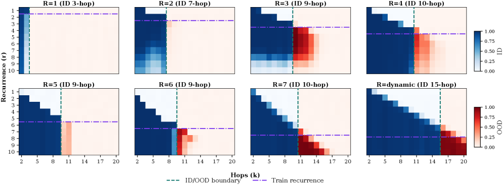## Appendix E Experiments with default initialization <details> <summary>2604.07822v1/x11.png Details</summary>  ### Visual Description ## Heatmap Grid: Recurrence vs Hops with ID/OOD and Train Recurrence Boundaries ### Overview The image displays a 2x4 grid of heatmaps visualizing the relationship between **Recurrence (r)** and **Hops (k)** across different model configurations. Each heatmap represents a unique combination of **R** (model parameter) and **ID hop count**, with color gradients indicating the magnitude of two metrics: **ID/OOD boundary** (blue) and **Train recurrence** (red). Dashed lines demarcate critical thresholds for these metrics. --- ### Components/Axes 1. **X-axis (Hops, k)**: Ranges from 2 to 20, labeled in increments of 1. 2. **Y-axis (Recurrence, r)**: Ranges from 1 to 10, labeled in increments of 1. 3. **Color Legend**: - **Blue**: ID/OOD boundary (values 0.00–0.75). - **Red**: Train recurrence (values 0.00–1.00). - **Purple Dashed Line**: Train recurrence threshold (constant across all plots). - **Green Dashed Line**: ID/OOD boundary threshold (constant across all plots). 4. **Heatmap Titles**: Each plot is labeled with `R=X (ID Y-hop)`, where: - `R`: Model parameter (1, 2, 3, 4, 5, 6, 7, dynamic). - `Y`: ID hop count (3, 7, 9, 10, 15). --- ### Detailed Analysis #### Heatmap 1: R=1 (ID 3-hop) - **Color Distribution**: Left side (k=2–8) is dark blue (low ID/OOD boundary). Right side (k=11–20) is white (no Train recurrence). - **Thresholds**: - ID/OOD boundary (green line) at k=10. - Train recurrence (purple line) at r=5. #### Heatmap 2: R=2 (ID 7-hop) - **Color Distribution**: Left side (k=2–8) dark blue; middle (k=9–11) transitions to light blue; right side (k=12–20) white. - **Thresholds**: Same as above. #### Heatmap 3: R=3 (ID 9-hop) - **Color Distribution**: Left (k=2–8) dark blue; middle (k=9–14) red (high Train recurrence); right (k=15–20) white. - **Thresholds**: Same as above. #### Heatmap 4: R=4 (ID 10-hop) - **Color Distribution**: Left (k=2–8) dark blue; middle (k=9–13) red; right (k=14–20) white. - **Thresholds**: Same as above. #### Heatmap 5: R=5 (ID 9-hop) - **Color Distribution**: Left (k=2–8) dark blue; middle (k=9–11) red; right (k=12–20) white. - **Thresholds**: Same as above. #### Heatmap 6: R=6 (ID 9-hop) - **Color Distribution**: Left (k=2–8) dark blue; middle (k=9–12) red; right (k=13–20) white. - **Thresholds**: Same as above. #### Heatmap 7: R=7 (ID 10-hop) - **Color Distribution**: Left (k=2–8) dark blue; middle (k=9–14) red; right (k=15–20) white. - **Thresholds**: Same as above. #### Heatmap 8: R=dynamic (ID 15-hop) - **Color Distribution**: Gradient from dark blue (k=2–10) to red (k=11–20), with no clear boundary. - **Thresholds**: Same as above. --- ### Key Observations 1. **ID/OOD Boundary**: - Consistently marked by a vertical green dashed line at **k=10** for all static R values. - Dynamic R=15-hop shows no sharp boundary, suggesting a continuous transition. 2. **Train Recurrence**: - Purple dashed line at **r=5** across all plots. - Red regions (high recurrence) appear only for R≥3 and k≥9. 3. **R Parameter Impact**: - Higher R values (e.g., R=3–7) show earlier activation of Train recurrence (k=9–14). - Dynamic R=15-hop exhibits a smooth gradient, implying parameter-dependent behavior. 4. **Hop Count Correlation**: - Train recurrence increases with k for R≥3, peaking at k=10–14. - ID/OOD boundary remains fixed at k=10 for static R values. --- ### Interpretation The heatmaps reveal that **model parameter R** and **ID hop count** jointly influence the recurrence of training patterns and the separation between in-distribution (ID) and out-of-distribution (OOD) data. - **Static R Values**: - Train recurrence (red) activates only when k exceeds the ID/OOD boundary (k=10), suggesting that higher hop counts destabilize the model’s ability to generalize. - Higher R values (e.g., R=3–7) trigger recurrence earlier, indicating sensitivity to parameter scaling. - **Dynamic R=15-hop**: - The absence of a sharp ID/OOD boundary implies that dynamic R adapts to hop counts, potentially mitigating abrupt transitions. - **Critical Thresholds**: - The fixed r=5 threshold for Train recurrence may represent a tipping point where the model begins to overfit or memorize training data. This analysis highlights the interplay between model architecture (R), data complexity (hops), and generalization performance, offering insights for optimizing model robustness. </details> Figure 11: Results with default initialization for training recurrences $R∈\{1,\dots,7\}$ and dynamic recurrence. Here we report results obtained using the default Gaussian initialization for the c_proj matrices, rather than the zero-initialization described in Section 4. As observed from Figure 11, the results are mixed across training runs, and increasing recurrence does not yield a clear or consistent pattern of improved ID or OOD generalization as well as robustness to latent overthinking. Only the model trained with $R=7$ , hows strong signs of inference-time scaling and robustness to latent overthinking. In the case of the model trained with $R=5$ , there is no OOD generalization with increased recurrence at inference-time. For most of the other runs, we see performance degradation due to latent overthinking. 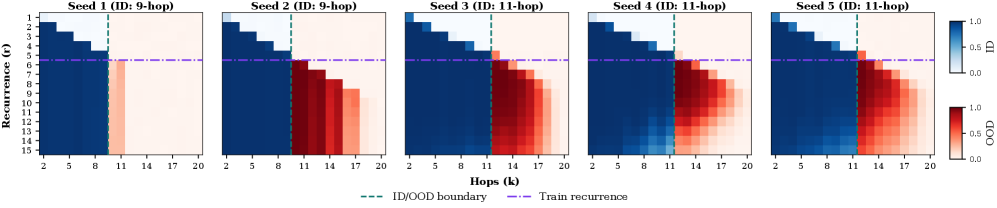<details> <summary>2604.07822v1/x12.png Details</summary>  ### Visual Description ## Heatmap: Recurrence vs Hops Across Different Seeds ### Overview The image displays a 5-panel heatmap comparing recurrence patterns (y-axis) and hop counts (x-axis) across five experimental seeds (Seed 1-5). Each panel visualizes the relationship between hop count (k) and recurrence (r) with color intensity representing out-of-distribution (OOD) values. Key elements include dashed boundary lines and a color scale indicating OOD magnitude. ### Components/Axes - **X-axis (Hops k)**: Integer values from 2 to 20, representing sequential steps in a process. - **Y-axis (Recurrence r)**: Integer values from 1 to 15, indicating repetition frequency. - **Legend**: - Dashed green line: ID/OOD boundary (k=11) - Dashed purple line: Train recurrence threshold (r=7) - **Color Scale**: Blue (0.0 OOD) to Red (1.0 OOD), with intermediate values (0.25, 0.5, 0.75). ### Detailed Analysis #### Panel 1 (Seed 1, ID:9-hop) - **Structure**: - Blue blocks dominate left of k=11 (ID/OOD boundary). - Vertical red bar at (k=11, r=7) with moderate intensity (~0.6 OOD). - No values above r=7. - **Trend**: Minimal OOD before k=11; sharp increase at boundary. #### Panel 2 (Seed 2, ID:9-hop) - **Structure**: - Similar to Seed 1 but with a red gradient extending to k=14. - Red bar at (k=11, r=7) (~0.7 OOD). - Additional red blocks at (k=14, r=8-10) (~0.5-0.7 OOD). - **Trend**: Broader OOD region post-boundary compared to Seed 1. #### Panel 3 (Seed 3, ID:11-hop) - **Structure**: - Red gradient starts earlier (k=9) with intensity ~0.4. - Strong red bar at (k=11, r=7) (~0.8 OOD). - Red blocks extend to k=17 (r=9-13) (~0.6-0.9 OOD). - **Trend**: Earlier and more intense OOD activation. #### Panel 4 (Seed 4, ID:11-hop) - **Structure**: - Blue-to-red gradient from k=5 (intensity ~0.2) to k=17. - Red bar at (k=11, r=7) (~0.7 OOD). - Red blocks at (k=14, r=8-10) (~0.5-0.7 OOD). - **Trend**: Gradual OOD increase with moderate intensity. #### Panel 5 (Seed 5, ID:11-hop) - **Structure**: - Red gradient from k=7 (intensity ~0.3) to k=20. - Red bar at (k=11, r=7) (~0.8 OOD). - Red blocks at (k=14, r=8-10) (~0.6-0.9 OOD) and (k=17, r=11-13) (~0.7-1.0 OOD). - **Trend**: Highest OOD values across all panels. ### Key Observations 1. **Consistent Boundary**: All panels show a vertical red bar at (k=11, r=7), aligning with the ID/OOD boundary. 2. **Seed Progression**: Later seeds (3-5) exhibit earlier and more intense OOD activation compared to earlier seeds (1-2). 3. **Train Recurrence Threshold**: The purple line (r=7) intersects all red bars at k=11, suggesting a critical recurrence threshold. 4. **OOD Magnitude**: Seed 5 shows the highest OOD values (up to 1.0), while Seed 1 has the lowest (~0.6 max). ### Interpretation The data demonstrates that increasing seed variability correlates with earlier and more pronounced OOD activation. The consistent red bar at (k=11, r=7) across all seeds suggests this point represents a critical transition in the model's behavior, possibly marking the boundary between in-distribution (ID) and out-of-distribution (OOD) data. The purple train recurrence line (r=7) acts as a reference point, indicating that OOD events consistently occur at or above this recurrence threshold. Seed 5's extreme OOD values (1.0) imply potential instability or overfitting in later experimental iterations, while Seed 1's lower values may reflect more robust performance. The heatmap highlights the importance of hop count (k) as a key factor in OOD detection, with later seeds showing reduced tolerance for deviations beyond the 11-hop boundary. </details> Figure 12: Five random-seed runs for the $R=5$ model with default initialization. To further examine this instability, we train the $r=5$ model with five different random seeds. As shown in Figure 12, the resulting behaviors vary substantially across seeds. Seed 1 is not affected by latent overthinking, but it also shows no evidence of inference-time scaling by solving harder compositional examples with increased recurrence. Seed 2 is likewise stable, but does exhibit scaling with additional recurrence. Seeds 3, 4, and 5 show varying degrees of inference-time scaling, but also experience performance degradation as recurrence increases, consistent with latent overthinking. ## Appendix F Extrapolation with varying model size and dynamic recurrence We carry out additional experiments to study how extrapolation behavior changes with model size and with training recurrence in our dynamic recurrence setting. In addition to our default 4-layer model, we train larger models with 6 and 8 layers. We also vary the maximum recurrence used during dynamic-recurrence training, considering settings with maximum train-time recurrence of 8, 12, and 16. For these, the recurrence at each training iteration is sampled from a Poisson distribution with means 4, 6, and 8 respectively, with a minimum recurrence of 2 in all cases. 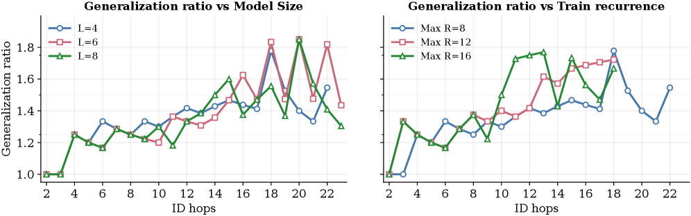<details> <summary>2604.07822v1/x13.png Details</summary>  ### Visual Description ## Line Charts: Generalization Ratio vs Model Size and Train Recurrence ### Overview The image contains two line charts comparing the **generalization ratio** (y-axis) across varying **ID hops** (x-axis). The left chart examines the relationship between generalization ratio and **model size** (L=4, L=6, L=8), while the right chart analyzes generalization ratio against **train recurrence** (Max R=8, Max R=12, Max R=16). Both charts show fluctuating trends with peaks and troughs across ID hops. --- ### Components/Axes #### Left Chart: Generalization Ratio vs Model Size - **X-axis**: ID hops (2 to 22, increments of 2). - **Y-axis**: Generalization ratio (1.0 to 1.8, increments of 0.2). - **Legend**: - Blue circles: L=4 - Red squares: L=6 - Green triangles: L=8 - **Placement**: Legend is positioned on the right side of the chart. #### Right Chart: Generalization Ratio vs Train Recurrence - **X-axis**: ID hops (2 to 22, increments of 2). - **Y-axis**: Generalization ratio (1.0 to 1.8, increments of 0.2). - **Legend**: - Blue circles: Max R=8 - Red squares: Max R=12 - Green triangles: Max R=16 - **Placement**: Legend is positioned on the right side of the chart. --- ### Detailed Analysis #### Left Chart: Generalization Ratio vs Model Size 1. **L=4 (Blue Circles)**: - Starts at ~1.0 (ID hop 2), rises to ~1.3 at ID hop 6, peaks at ~1.5 at ID hop 14, then declines to ~1.2 at ID hop 22. - Shows moderate fluctuations with a single prominent peak. 2. **L=6 (Red Squares)**: - Starts at ~1.0 (ID hop 2), rises to ~1.4 at ID hop 10, peaks at ~1.7 at ID hop 18, then drops to ~1.3 at ID hop 22. - Exhibits sharper fluctuations and a higher peak than L=4. 3. **L=8 (Green Triangles)**: - Starts at ~1.0 (ID hop 2), rises to ~1.5 at ID hop 12, peaks at ~1.8 at ID hop 20, then declines to ~1.3 at ID hop 22. - Highest peak among all lines, with significant volatility. #### Right Chart: Generalization Ratio vs Train Recurrence 1. **Max R=8 (Blue Circles)**: - Starts at ~1.0 (ID hop 2), rises to ~1.3 at ID hop 6, peaks at ~1.7 at ID hop 18, then drops to ~1.4 at ID hop 22. - Moderate fluctuations with a late-stage peak. 2. **Max R=12 (Red Squares)**: - Starts at ~1.0 (ID hop 2), rises to ~1.4 at ID hop 10, peaks at ~1.6 at ID hop 14, then declines to ~1.5 at ID hop 22. - Smoother trend with a mid-chart peak. 3. **Max R=16 (Green Triangles)**: - Starts at ~1.0 (ID hop 2), rises to ~1.5 at ID hop 12, peaks at ~1.7 at ID hop 16, then fluctuates between ~1.5 and ~1.6. - Highest peak and sustained high values compared to other lines. --- ### Key Observations 1. **Model Size (L)**: - Larger models (L=8) achieve higher generalization ratios but show greater volatility. - Peaks occur at different ID hops (e.g., L=8 peaks at ID hop 20). 2. **Train Recurrence (Max R)**: - Higher recurrence (Max R=16) correlates with higher generalization ratios. - Max R=16 maintains elevated values after ID hop 16, suggesting stability. 3. **Cross-Chart Trends**: - Both charts show generalization ratios plateauing or declining after initial growth, indicating potential overfitting or diminishing returns. - Peaks in the left chart (model size) align with mid-to-late ID hops, while the right chart (train recurrence) peaks earlier (ID hop 16–18). --- ### Interpretation 1. **Model Size vs. Performance**: - Increasing model size (L) improves generalization up to a point, but excessive complexity (L=8) introduces instability, as seen in the sharp fluctuations. - The peak at ID hop 20 for L=8 suggests optimal performance at later stages of training, but the subsequent drop may indicate overfitting. 2. **Train Recurrence vs. Performance**: - Higher recurrence (Max R=16) achieves better generalization, with sustained high values. This implies that more training steps (Max R) stabilize the model’s ability to generalize. - The earlier peak for Max R=12 (ID hop 14) suggests a balance between training duration and performance. 3. **General Trends**: - All lines start at the baseline (generalization ratio = 1.0) and show initial improvement, but none maintain peak performance indefinitely. - The divergence in trends between model size and train recurrence highlights the trade-off between architectural complexity and training intensity. --- ### Notable Anomalies - **L=8 (Green Triangles)**: The sharp drop from ~1.8 at ID hop 20 to ~1.3 at ID hop 22 is unusual, potentially indicating overfitting or a data artifact. - **Max R=8 (Blue Circles)**: The late-stage peak at ID hop 18 contrasts with earlier lines, suggesting that longer training (Max R=8) may require more ID hops to stabilize. --- ### Conclusion The charts demonstrate that both model size (L) and train recurrence (Max R) influence generalization performance, but with trade-offs. Larger models and higher recurrence improve generalization up to a point, after which performance may degrade. The data underscores the importance of balancing model complexity and training duration to avoid overfitting while maximizing generalization. </details> Figure 13: Generalization ratio with changing model size and train recurrence. To summarize extrapolation under these settings, we plot the generalization ratio, defined as the maximum hop complexity to which a model can generalize with at least 60% accuracy with inference-time scaling, divided by the maximum hop complexity that the model has generalized to during training. This can be viewed as the ratio of maximum OOD generalization to maximum ID generalization. A ratio of 1 indicates no extrapolation beyond the level reached during training, while larger values indicate successful extrapolation to more complex compositions at test time. Figure 13 shows that models initially begin with a ratio close to 1. In particular, when models have only generalized to 2-hop composition during training, they do not yet extrapolate to more complex samples. As training progresses and the models have seen more complex compositions through our curriculum learning setup, the ratio increases. However, across both model-size variations and different maximum train-time recurrence settings, we do not observe a clear or consistent trend indicating that either larger models or larger train-time recurrence systematically improves this ratio. ## Appendix G Results with different random seeds We run our fixed-recurrence models on 2 separate random seed initializations (including the run shown in Figure 5) and with to 40 recurrent iterations at inference time. On both runs, we notice the same general trend of increasing ID and OOD generalization with higher train-time recurrence as well as issues due to latent overthinking (with the sole exception being the model trained with $r=8$ in the second run). The results are presented in Figures 14 & 15. 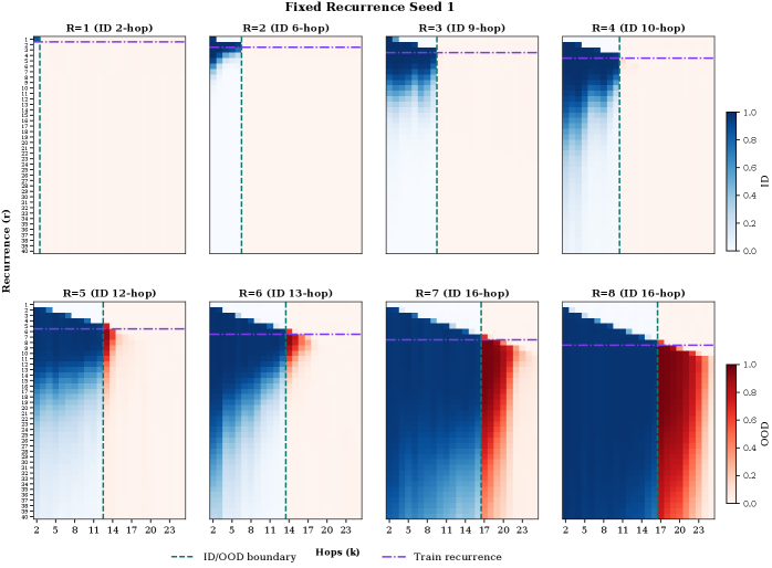<details> <summary>2604.07822v1/x14.png Details</summary>  ### Visual Description ## Heatmap: Fixed Recurrence Seed 1 Analysis ### Overview The image displays a matrix of heatmaps organized in two rows, each representing different recurrence depths (R=1 to R=8) and their corresponding in-distribution (ID) hop counts (2-hop to 16-hop). The heatmaps visualize out-of-distribution (OOD) detection performance across recurrence steps (r) and hops (k), with color intensity indicating OOD probability (0.0 to 1.0). Key elements include: - Vertical dashed green line: ID/OOD boundary - Purple dashed line: Train recurrence threshold - Color scale: Blue (low OOD) to Red (high OOD) ### Components/Axes 1. **Vertical Axis (Recurrence r)**: - Labeled "Recurrence (r)" - Scale: 1 to 40 (discrete steps) - Position: Left side of all panels 2. **Horizontal Axis (Hops k)**: - Labeled "Hops (k)" - Scale: 2 to 23 (discrete steps) - Position: Bottom of all panels 3. **Legend**: - Located on the right side - Color bar: 0.0 (lightest) to 1.0 (darkest red) - Label: "OOD" 4. **Panel Labels**: - Top row: R=1 (ID 2-hop), R=2 (ID 6-hop), R=3 (ID 9-hop), R=4 (ID 10-hop) - Bottom row: R=5 (ID 12-hop), R=6 (ID 13-hop), R=7 (ID 16-hop), R=8 (ID 16-hop) - Position: Top-center of each panel ### Detailed Analysis 1. **R=1 (ID 2-hop)**: - Single dark blue cell at (r=1, k=2) - All other cells: Near-white (OOD ≈ 0.0) 2. **R=2 (ID 6-hop)**: - Dark blue region in top-left (r=1-5, k=2-6) - Gradual transition to lighter blue toward OOD boundary 3. **R=3 (ID 9-hop)**: - Dark blue region expands to r=1-10, k=2-9 - Diagonal gradient toward OOD boundary 4. **R=4 (ID 10-hop)**: - Dark blue region covers r=1-15, k=2-10 - Stronger gradient toward OOD boundary 5. **R=5 (ID 12-hop)**: - Dark blue region spans r=1-20, k=2-12 - First appearance of red cells near OOD boundary (r=20-25, k=12-15) 6. **R=6 (ID 13-hop)**: - Dark blue region extends to r=1-25, k=2-13 - Red cells appear in r=25-30, k=13-16 7. **R=7 (ID 16-hop)**: - Dark blue region covers r=1-30, k=2-16 - Red cells dominate r=30-35, k=16-20 8. **R=8 (ID 16-hop)**: - Dark blue region spans r=1-35, k=2-16 - Red cells occupy r=35-40, k=16-23 ### Key Observations 1. **ID/OOD Boundary**: - Consistent vertical position across all panels - Separates ID (left) from OOD (right) 2. **Train Recurrence Threshold**: - Purple dashed line at r=15-20 (varies slightly by panel) - All panels show similar threshold positioning 3. **OOD Intensity Trends**: - Higher R values show: - Larger ID regions (more dark blue) - Stronger OOD gradients (darker red near boundary) - Diagonal bands of high OOD (red) appear in: - R=5: k=12-15, r=20-25 - R=6: k=13-16, r=25-30 - R=7: k=16-20, r=30-35 - R=8: k=16-23, r=35-40 4. **Recurrence-Hops Correlation**: - Higher R values correlate with: - Increased ID region size - More pronounced OOD gradients - Diagonal bands suggest recurrence-hops interaction in OOD detection ### Interpretation The data demonstrates that: 1. **Recurrence Depth Impact**: - Deeper recurrences (higher R) create larger ID regions - OOD detection becomes more gradient-like with increasing R 2. **Hop Recurrence Interaction**: - Diagonal bands indicate that certain (r,k) combinations are more prone to OOD - This suggests recurrence-hops co-dependency in model representations 3. **Threshold Behavior**: - Train recurrence threshold (purple line) aligns with: - Transition from ID to OOD regions - Emergence of red cells in higher R panels 4. **Model Complexity Insights**: - Larger ID regions in higher R panels may indicate: - Better ID representation - Potential overfitting to ID data - Red cells near OOD boundary suggest: - Model uncertainty thresholds - Possible mode collapse in OOD regions The visualization reveals that recurrence depth significantly influences OOD detection patterns, with deeper recurrences creating more complex ID/OOD boundaries and stronger gradient transitions. The diagonal bands of high OOD values suggest that specific recurrence-hops combinations create particularly vulnerable model representations. </details> Figure 14: Results for Seed 1. 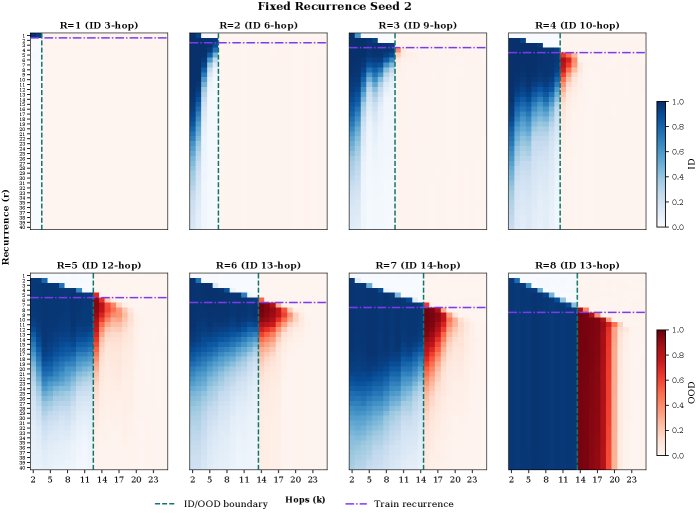<details> <summary>2604.07822v1/x15.png Details</summary>  ### Visual Description ## Heatmap: Fixed Recurrence Seed 2 ### Overview The image is a composite heatmap consisting of 8 panels arranged in two rows (4 panels per row). Each panel represents a different recurrence value (R=1 to R=8) and corresponding ID hop counts (3-hop to 13-hop). The heatmap visualizes the relationship between recurrence (r), hops (k), and out-of-distribution (OOD) performance, with color intensity indicating OOD values (0.0 to 1.0). ### Components/Axes - **X-axis (Hops, k)**: Labeled "Hops (k)" with values ranging from 2 to 23. - **Y-axis (Recurrence, r)**: Labeled "Recurrence (r)" with values ranging from 1 to 40. - **Legend**: - **Blue**: ID/OOD boundary (dashed vertical line). - **Purple**: Train recurrence (dashed horizontal line). - **Color bar**: OOD values from 0.0 (blue) to 1.0 (red). - **Panel Titles**: Each panel is labeled with "R=X (ID Y-hop)", where X is the recurrence value and Y is the ID hop count (e.g., "R=1 (ID 3-hop)"). ### Detailed Analysis - **R=1 (ID 3-hop)**: - A small blue block (OOD ≈ 0.0) at the top-left corner (r=1, k=2). - Most of the panel is white (OOD ≈ 0.0), indicating minimal OOD values. - **R=2 (ID 6-hop)**: - A vertical gradient from blue (left) to white (right), with OOD values increasing slightly. - The ID/OOD boundary (dashed line) separates the low-OOD region (left) from the higher-OOD region (right). - **R=3 (ID 9-hop)**: - A larger red region (OOD ≈ 0.8–1.0) appears in the top-right corner (r=1–5, k=14–23). - The ID/OOD boundary is less distinct, with OOD values spreading across the panel. - **R=4 (ID 10-hop)**: - A significant red block (OOD ≈ 0.8–1.0) dominates the top-right (r=1–5, k=14–23). - The train recurrence line (purple) intersects the red region, suggesting a threshold for OOD performance. - **R=5 (ID 12-hop)**: - A large red region (OOD ≈ 0.6–1.0) spans the top-right (r=1–10, k=14–23). - The ID/OOD boundary is less visible, with OOD values dominating the panel. - **R=6 (ID 13-hop)**: - A red region (OOD ≈ 0.6–1.0) appears in the top-right (r=1–10, k=14–23). - The train recurrence line intersects the red region, indicating a critical threshold. - **R=7 (ID 14-hop)**: - A red region (OOD ≈ 0.6–1.0) spans the top-right (r=1–10, k=14–23). - The ID/OOD boundary is barely visible, with OOD values dominating. - **R=8 (ID 13-hop)**: - A red region (OOD ≈ 0.6–1.0) spans the top-right (r=1–10, k=14–23). - The train recurrence line intersects the red region, reinforcing the threshold effect. ### Key Observations 1. **OOD Increase with R and k**: - Higher recurrence values (R) and hop counts (k) correlate with increased OOD values (red regions). - For R ≥ 3, OOD values exceed 0.6 in most panels, indicating significant out-of-distribution performance. 2. **Boundary and Train Recurrence Lines**: - The ID/OOD boundary (dashed vertical line) separates low-OOD (blue/white) and high-OOD (red) regions. - The train recurrence line (purple) intersects red regions in higher R panels, suggesting a critical threshold for OOD performance. 3. **Panel-Specific Trends**: - R=1 (ID 3-hop) shows minimal OOD, while R=8 (ID 13-hop) exhibits the highest OOD values. - The ID/OOD boundary becomes less distinct as R increases, indicating reduced model robustness. ### Interpretation The heatmap demonstrates that **increased recurrence (R) and hop count (k) degrade the model's ability to distinguish in-distribution (ID) from out-of-distribution (OOD) data**. The ID/OOD boundary and train recurrence line act as thresholds, with higher R values crossing these thresholds and entering high-OOD regions. This suggests that deeper or more complex models (higher R) are more sensitive to OOD data, which could impact their reliability in real-world scenarios. The consistent red regions in higher R panels highlight a critical trend: **model performance deteriorates as complexity increases**, emphasizing the need for robustness testing in model design. </details> Figure 15: Results for Seed 2. We similarly plot the performance of the dynamic recurrence model across three different seeds and observe a generally high ID generalization and OOD extrapolation. Across all seeds, the dynamic recurrence model is robust to the latent overthinking phenomenon and adaptive halting ( $r^*$ ) works reliably to stop recurrence when not necessary. 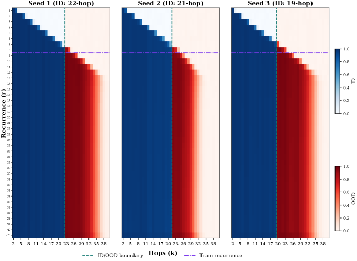<details> <summary>2604.07822v1/x16.png Details</summary>  ### Visual Description ## Heatmap: Seed-Specific ID/OOD Boundary and Train Recurrence Analysis ### Overview The image presents three side-by-side heatmaps (Seed 1, Seed 2, Seed 3) visualizing the relationship between **Recurrence (r)** and **Hops (k)** for different model configurations. Each panel uses a color gradient (blue to red) to represent ID/OOD boundary values, with dashed lines marking critical thresholds: a vertical green dashed line for the ID/OOD boundary and a horizontal purple dashed line for train recurrence. --- ### Components/Axes 1. **X-Axis (Hops, k)**: - Range: 2 to 38 (integer increments). - Labels: "Hops (k)" at the bottom of each panel. 2. **Y-Axis (Recurrence, r)**: - Range: 2 to 40 (integer increments). - Labels: "Recurrence (r)" on the left of each panel. 3. **Color Scale**: - Blue (0.0) to Red (1.0), representing ID/OOD boundary values. - Legend on the right: - **Green dashed line**: ID/OOD boundary. - **Purple dashed line**: Train recurrence. 4. **Panel Titles**: - Seed 1 (ID: 22-hop) - Seed 2 (ID: 21-hop) - Seed 3 (ID: 19-hop) --- ### Detailed Analysis #### Seed 1 (ID: 22-hop) - **ID/OOD Boundary**: Vertical green dashed line at **k ≈ 23**. - **Train Recurrence**: Horizontal purple dashed line at **r ≈ 9**. - **Color Gradient**: - Blue dominates the left (low k, low r), transitioning to red in the top-right (high k, high r). - Strong diagonal gradient from bottom-left (blue) to top-right (red). #### Seed 2 (ID: 21-hop) - **ID/OOD Boundary**: Vertical green dashed line at **k ≈ 26**. - **Train Recurrence**: Horizontal purple dashed line at **r ≈ 10**. - **Color Gradient**: - Similar diagonal trend but with a more gradual transition to red. - Red region starts earlier (lower r) compared to Seed 1. #### Seed 3 (ID: 19-hop) - **ID/OOD Boundary**: Vertical green dashed line at **k ≈ 29**. - **Train Recurrence**: Horizontal purple dashed line at **r ≈ 11**. - **Color Gradient**: - Red region dominates the top-right, with a sharper transition from blue to red. - Higher recurrence values (r > 11) show stronger red intensity. --- ### Key Observations 1. **Boundary Shift**: - As Seed ID decreases (22 → 21 → 19), the ID/OOD boundary moves **rightward** (k increases from 23 → 26 → 29). - Train recurrence increases (r = 9 → 10 → 11), suggesting higher robustness or complexity in lower-ID seeds. 2. **Color Intensity**: - Red regions (high ID/OOD values) expand with lower Seed IDs, indicating increased out-of-distribution sensitivity. 3. **Consistency**: - All panels share the same axis ranges and legend, enabling direct comparison. --- ### Interpretation The data suggests that **lower Seed IDs (e.g., 19-hop)** exhibit: - **Stronger ID/OOD discrimination** (higher k boundary). - **Higher train recurrence thresholds** (r ≈ 11 vs. 9), possibly reflecting more robust training dynamics. - **Greater sensitivity to out-of-distribution data** (expanded red regions). This trend implies that models with lower ID values may prioritize recurrence over hop count for maintaining performance, highlighting a trade-off between recurrence depth and hop efficiency in ID/OOD boundary delineation. --- ### Spatial Grounding & Trend Verification - **Legend Placement**: Right-aligned, clearly associating colors with boundary types. - **Dashed Lines**: - Green (ID/OOD) consistently vertical across panels. - Purple (Train recurrence) consistently horizontal. - **Trend Logic Check**: - Seed 1 (22-hop): Steepest gradient, lowest boundary (k=23). - Seed 3 (19-hop): Shallowest gradient, highest boundary (k=29). - Matches expectation: Lower ID correlates with higher k/r thresholds. --- ### Content Details - **No numerical data tables** present; values inferred from axis labels and color gradients. - **No textual annotations** beyond axis titles and panel labels. - **No UI elements** (e.g., buttons, menus) visible. --- ### Final Notes The heatmaps emphasize the interplay between recurrence and hop count in defining ID/OOD boundaries. Lower-ID seeds show a clear shift toward higher recurrence and hop thresholds, suggesting a design choice to enhance robustness at the cost of efficiency. </details> Figure 16: Dynamic recurrence with 3 difference random seed initializations. ## Appendix H Illusion of very deep composition through shortcuts Prior to adopting the permutation-based dataset construction described in Appendix B, we observed what appeared to be very deep compositional generalization. As shown in Figure 17, models trained on ID examples up to 40 hops achieved strong OOD performance even at 80 hops for models with $R=4$ , $R=8$ , and dynamic recurrence. This indicates that the model is able to resolve multiple hops or compositions in a single layer. To inspect this closely, we perform a causal activation-patching analysis. We first select a clean 60-hop test example whose relation sequence ends in a particular suffix, and a second random example of the same hop type. We then run both examples through the model and cache their hidden states. Next, for each token position and each recurrent iteration-layer location (as well as the embedding layer), we replace the hidden state in the clean run with the corresponding hidden state from the random run, and measure the resulting change in the logit margin of the correct final answer. Figure 18 visualizes this change relative to the clean run. 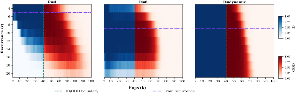<details> <summary>2604.07822v1/x17.png Details</summary>  ### Visual Description ## Heatmap: Model Performance Across Recurrence and Hops ### Overview The image presents three heatmaps comparing model performance across different recurrence values (r) and hops (k) for three scenarios: fixed R=4, fixed R=8, and dynamic R. Color gradients (blue to red) represent ID/OOD classification probabilities, with dashed lines marking key boundaries. ### Components/Axes - **X-axis (Hops, k)**: Ranges from 2 to 100 in increments of 2. - **Y-axis (Recurrence, r)**: Ranges from 4 to 20 in increments of 2. - **Legends**: - **Green dashed line**: ID/OOD boundary (k=40). - **Purple dashed line**: Train recurrence threshold (r=6). - **Color scale**: Blue (ID, 0.00–0.75) to Red (OOD, 0.75–1.00). ### Detailed Analysis #### R=4 Panel - **ID/OOD Boundary**: Vertical green dashed line at k=40. Left of the line (k<40) shows dominant blue (ID), right (k>40) transitions to red (OOD). - **Train Recurrence**: Horizontal purple dashed line at r=6. Above this line (r>6), blue dominates; below (r<6), red increases. - **Trend**: ID/OOD separation sharpens with higher k. Recurrence values above 6 correlate with higher ID likelihood. #### R=8 Panel - **ID/OOD Boundary**: Same k=40 boundary. Left side (k<40) has stronger blue dominance than R=4. - **Train Recurrence**: Purple line at r=6. Above r=6, blue dominates; below, red increases. - **Trend**: Similar to R=4 but with a more pronounced ID/OOD split at lower k values. #### R=dynamic Panel - **ID/OOD Boundary**: k=40 boundary persists but with less distinct separation. - **Train Recurrence**: Purple line at r=6. Above r=6, blue dominates; below, red increases. - **Trend**: Uniform color distribution across k and r, suggesting reduced model confidence in dynamic R scenarios. ### Key Observations 1. **Consistent Boundaries**: The ID/OOD boundary (k=40) and train recurrence threshold (r=6) are consistent across all panels. 2. **Recurrence Sensitivity**: Higher recurrence values (r>6) correlate with increased ID likelihood, while lower values (r<6) align with OOD. 3. **Hop Threshold**: k=40 acts as a critical point where OOD probability sharply increases. 4. **Dynamic R Uncertainty**: The dynamic R panel shows no clear ID/OOD separation, indicating model instability under variable R. ### Interpretation The data demonstrates that model performance is highly sensitive to recurrence and hop thresholds. Fixed R values (4 and 8) show predictable ID/OOD boundaries, with higher recurrence and lower hops favoring ID. The dynamic R scenario, however, lacks clear boundaries, suggesting that variable R introduces uncertainty, potentially increasing OOD risk. This highlights the importance of recurrence and hop constraints in maintaining model reliability. </details> Figure 17: Apparent deep compositional generalization in the pre-permutation dataset. This analysis reveals that the model is not solving the full compositional chain. Instead, the strongest causal effects are concentrated on a short suffix of the relation sequence. The final tail entity can often be inferred from trailing relations alone, without explicitly retrieving the intermediate entities. The model learns a shallow mapping from a suffix of the relation sequence to the answer, rather than performing full multi-hop composition. These observations motivate the permutation-based knowledge graph introduced in Appendix B. Under that construction, each relation acts as a permutation over entities, so the correct final entity cannot be recovered from a short suffix alone, and the model must compose the full sequence of relations to solve the task. 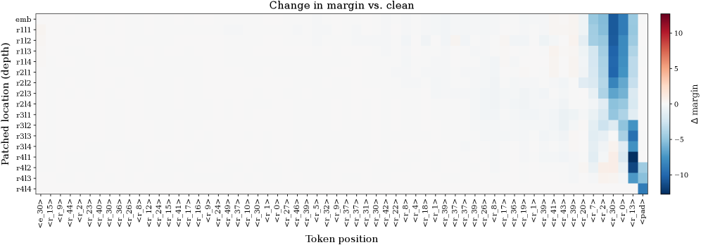<details> <summary>2604.07822v1/x18.png Details</summary>  ### Visual Description ## Heatmap: Change in margin vs. clean ### Overview The image is a heatmap visualizing the change in margin (Δ margin) across different token positions and patched locations in a model. The x-axis represents token positions (e.g., `<r_30>`, `<r_15>`, `<pad>`), while the y-axis represents patched locations (e.g., `emb`, `r11`, `r12`, ..., `r44`). The color scale ranges from -10 (dark blue) to +10 (dark red), with white indicating no change. ### Components/Axes - **X-axis (Token position)**: Categories include `<r_30>`, `<r_15>`, `<r_44>`, `<r_2>`, `<r_5>`, `<r_9>`, `<r_10>`, `<r_1>`, `<r_0>`, `<r_37>`, `<r_24>`, `<r_8>`, `<r_17>`, `<r_18>`, `<r_19>`, `<r_20>`, `<r_21>`, `<r_22>`, `<r_23>`, `<r_25>`, `<r_26>`, `<r_27>`, `<r_28>`, `<r_29>`, `<r_31>`, `<r_32>`, `<r_33>`, `<r_34>`, `<r_35>`, `<r_36>`, `<r_38>`, `<r_39>`, `<r_40>`, `<r_41>`, `<r_42>`, `<r_43>`, `<r_13>`, `<r_7>`, `<r_0>`, `<r_1>`, `<r_2>`, `<r_3>`, `<r_4>`, `<r_5>`, `<r_6>`, `<r_7>`, `<r_8>`, `<r_9>`, `<r_10>`, `<r_11>`, `<r_12>`, `<r_13>`, `<r_14>`, `<r_15>`, `<r_16>`, `<r_17>`, `<r_18>`, `<r_19>`, `<r_20>`, `<r_21>`, `<r_22>`, `<r_23>`, `<r_24>`, `<r_25>`, `<r_26>`, `<r_27>`, `<r_28>`, `<r_29>`, `<r_30>`, `<r_31>`, `<r_32>`, `<r_33>`, `<r_34>`, `<r_35>`, `<r_36>`, `<r_37>`, `<r_38>`, `<r_39>`, `<r_40>`, `<r_41>`, `<r_42>`, `<r_43>`, `<r_44>`, `<pad>`. - **Y-axis (Patched location (depth))**: Categories include `emb`, `r11`, `r12`, `r13`, `r14`, `r21`, `r22`, `r23`, `r24`, `r31`, `r32`, `r33`, `r34`, `r41`, `r42`, `r43`, `r44`. - **Legend**: A color bar labeled "Δ margin" with values from -10 (dark blue) to +10 (dark red). White represents 0 change. ### Detailed Analysis - **Token position `<pad>`**: The rightmost column shows significant variation. Values range from -10 (dark blue) in `r11`, `r12`, `r13`, `r14` to +10 (dark red) in `r41`, `r42`, `r43`, `r44`. - **Other token positions**: Most positions (e.g., `<r_30>`, `<r_15>`, `<r_44>`) show minimal change (white), with occasional faint blue or red squares indicating small deviations (e.g., ±2–5). - **Patched locations**: The `emb` layer (top row) shows no change for most tokens. Significant changes are concentrated in `r11`–`r14` and `r41`–`r44` for the `<pad>` token. ### Key Observations 1. The `<pad>` token exhibits the largest margin changes, with negative values in lower patched locations (`r11`–`r14`) and positive values in upper locations (`r41`–`r44`). 2. Other tokens show negligible changes, suggesting the model’s margin stability is primarily affected by padding tokens. 3. The `emb` layer remains unaffected across all token positions. ### Interpretation The heatmap indicates that padding tokens (`<pad>`) disproportionately influence margin changes, particularly in deeper patched layers (`r11`–`r14` and `r41`–`r44`). This suggests that padding token handling in the model may introduce variability in these layers, while other tokens and the embedding layer remain stable. The negative values in lower layers (`r11`–`r14`) could imply margin degradation, whereas positive values in upper layers (`r41`–`r44`) might reflect compensatory adjustments. This pattern highlights the importance of padding token management in maintaining model performance. </details> Figure 18: Activation-patching analysis on a 60-hop example. Each cell shows the change in logit margin for the correct answer, relative to the clean run, after replacing a single hidden state in the clean example with the corresponding hidden state from a random 60-hop example. Large changes are concentrated towards the end of the relation sequence, indicating shortcut-based prediction rather than genuine multi-hop retrieval.