2604.08451v1

# Taming GPU Underutilization via Static Partitioning and Fine-grained CPU Offloading **Authors**: Gabin Schieffer, Ruimin Shi, Jie Ren, Ivy Peng ## Abstract Advances in GPU compute throughput and memory capacity brings significant opportunities to a wide range of workloads. However, efficiently utilizing these resources remains challenging, particularly because diverse application characteristics may result in imbalanced utilization. Multi-Instance GPU (MIG) is a promising approach to improve utilization by partitioning GPU compute and memory resources into fixed-size slices with isolation. Yet, its effectiveness and limitations in supporting HPC workloads remain an open question. We present a comprehensive system-level characterization of different GPU sharing options using real-world scientific, AI, and data analytics applications, including NekRS, LAMMPS, Llama3, and Qiskit. Our analysis reveals that while GPU sharing via MIG can significantly reduce resource underutilization, and enable system-level improvements in throughput and energy, interference still occurs through shared resources, such as power throttling. Our performance-resource scaling results indicate that coarse-grained provisioning for tightly coupled compute and memory resources often mismatches application needs. To address this mismatch, we propose a memory-offloading scheme that leverages the cache-coherent Nvlink-C2C interconnect to bridge the gap between coarse-grained resource slices and reduce resource underutilization. ## I Introduction The rapid growth of machine learning, scientific, and data analytics workloads has driven an unprecedented demand for GPU resources. For example, Large Language Models (LLM) require high memory capacity, bandwidth, and compute throughput to meet the performance target. On recent generations of GPU architectures, compute and memory resources are continuously increasing. For instance, in the latest four generations of Nvidia GPUs, GPU compute and memory capacity are evolving at a nearly doubling rate as summarized in Table I. While the increased GPU resources can generally benefit a wide range of workloads, the exact performance-resource scaling may differ in applications, depending on their characteristics. Consequently, their utilization of GPU resources may become suboptimal due to workload-specific characteristics in resource demands, raising the concern of under-utilization of GPU resources, which in turn undermines overall operating cost-efficiency of GPU systems [1, 2]. GPU sharing emerges as a promising approach to improve resource utilization by enabling multiple processes to concurrently run a single GPU [3, 1, 4, 5, 6, 7]. Two main GPU sharing schemes exist – temporal sharing and spatial sharing. Time slicing on Nvidia GPUs, for instance executes one process at a time on the GPU, switching among processes to create the illusion of multiple processes making progress at the same time. Spatial sharing partitions compute and memory resources among processes so that multiple processes can execute on the GPU concurrently. Common spatial sharing mechanisms include Multi-Process Service (MPS) [8], which partitions compute resources only, and the more recent Multi-Instance GPU (MIG), which partitions both compute and memory resources. These GPU sharing options provide different levels of isolation, flexibility, and resource overhead [9]. Many prior works have explored GPU sharing for machine learning workloads [10, 11, 5], but few have explored resource underutilization in HPC applications with a particular focus on the MIG mechanism [12, 7]. TABLE I: Characteristics of four generations of Nvidia GPUs. | | Memory | Throughput (TFLOPS) | | | | | --- | --- | --- | --- | --- | --- | | Capacity | Bandwidth | FP32 | Tensor (FP16) | SMs | | | V100 | 32 GB | 1.1 TB/s | 16.4 | 130 | 80 | | A100 | 80 GB | 2.0 TB/s | 19.5 | 312 | 108 | | H100 | 144 GB | 4.9 TB/s | 60 | 1000 | 132 | | B200 | 192 GB | 8.0 TB/s | 80 | 2500 | 160 | In this work, we focus on the impact of GPU sharing on resource underutilization, both regarding compute resources, in terms of the number of streaming multiprocessors (SMs), and memory resources, in terms of capacity and bandwidth. We compose a suite of eight real-world workloads, including Qiskit, LAMMPS, NekRS, Llama 3, and FAISS, to represent workloads in scientific, LLM, and data analytics domains. On a Nvidia Grace Hopper system, we collect a set of metrics pertaining to compute and memory resource underutilization, to assess the effectiveness of different GPU sharing options, such as MPS and MIG, in improving resource efficiency. Our results indicate that the coarse-grained resource provisioning of tightly coupled compute and memory resources in MIG profiles mismatches the resource-performance scaling characteristics in real applications. To address the coarse-grained resource provisioning in fixed MIG slices, we further explore leveraging Nvlink-C2C to selectively offload memory onto CPU, so that workloads slightly larger than a MIG slice can run without requiring a larger MIG slice. Since MIG slices increase compute and memory resources at a doubling rate, this offloading option improves the continuity in resource provisioning. Consequently, this approach can be used to address the problem of resource underutilization when resources can only be scaled at fixed configurations. To facilitate the choice of a suitable MIG configuration for GPU sharing, we further propose a new reward metric that trades off system-level throughput and resource underutilization for different priorities. We use this metric to assess the opportunity of using memory offloading in tested applications. In summary, we made the following contributions in this work: - We provide a method for quantifying resource underutilization in different GPU sharing schemes, including MIG, MPS, and time-slicing and apply it to a set of real-world applications from LLM, HPC and data analytics domains; - We identify the opportunities of GPU sharing in improving system throughput and energy, and power throttling as the main interference challenge; - We propose a memory offloading scheme over Nvlink-C2C as a solution to tackle resource underutilization in MIG; - We define a reward metric that trades off performance and resource underutilization for selecting GPU sharing configurations to meet different targets. ## II Motivation and Background ### II-A Single Application GPU Sharing In CUDA on Nvidia GPUs, submitting work to the GPU is done through CUDA stream [13]. A stream is an ordered queue of commands, e.g., data movement commands, synchronization commands, and GPU kernel launch commands. Commands submitted to two distinct streams might execute concurrently on the GPU, enabling some level of concurrency within a single application that uses multiple streams. Green contexts are lightweight CUDA contexts that can be configured to only execute kernels on a fixed set of the GPU’s SMs [14], offering more granular control over CUDA streams. By creating two or more green contexts, applications can control the mapping of GPU kernels to SMs [10]. For example, an application can create two green contexts, one with 16 SMs and another one with 32 SMs, and execute two kernels concurrently on distinct sets of SMs. ### II-B Multi-Application GPU Sharing This type of GPU sharing aims at providing several processes with concurrent access to a single physical GPU. Two main GPU sharing schemes can be identified. First temporal sharing, where the GPU only executes work submitted by one process at a time, switching between processes to provide the illusion of the processes simultaneously executing work on the GPU. The second scheme, spatial sharing, distributed GPU compute resources to concurrently executes computational work from several processes. At the system level, spatial sharing can be achieved through Multi-Process Service (MPS), which partition compute resources, but keeps GPU memory resources and L2 cache shared between processes; and Multi-Instance GPU (MIG), which partitions both compute and memory resources. #### II-B 1 Time-slicing By default, each process on a GPU-accelerated system maintains its own GPU context. The default scheduling strategy, referred to a time-slicing, schedules GPU kernels submitted by distinct processes to the GPU in a round-robin fashion. When a process whishes to submit a GPU kernel to the GPU, it is given a fixed amount of time to execute on the whole GPU. The context switching between processes comes with a significant performance cost, as no computational work is executed on the GPU during the context switch. With time-slicing, GPU kernels from distinct processes never execute simultaneously on the GPU, however, other operations, such as data copy operations might execute concurrently. #### II-B 2 Multi-Process Service (MPS) Multi-Process Service (MPS) [8] is a software mechanism to provide spatial sharing. One process, the MPS server, maintains a GPU context and regular CUDA applications submit work to the GPU through the server, effectively sharing one GPU context across independent processes. MPS executes GPU kernels submitted by each client on a portion of the GPU streaming multiprocessors (SM), effectively achieving spatial sharing of the GPU’s compute resources. The amount of SMs allocated to each process is controlled by the user as a percentage of the total SM count. On Volta GPUs and newer, MPS provides memory segmentation between processes. However, the memory capacity, bandwidth, and L2 cache are always shared between processes and thus, memory interference may occur. Moreover, MPS does not provide error isolation. When a GPU kernel in one MPS process generates a fatal GPU fault, all other processes’ GPU kernels executing at the same time on the GPU also return with an error. This specificity makes MPS unsuitable for multi-user GPU sharing. #### II-B 3 Multi-instance GPU <details> <summary>2604.08451v1/x1.png Details</summary>  ### Visual Description ## Diagram: NVIDIA H100 GPU Architecture ### Overview The diagram illustrates the hierarchical structure of an NVIDIA H100 GPU, showcasing its memory hierarchy, compute units, and interconnects. Key components include GPU memory, HBM3 modules, memory buses, L2 cache, streaming multiprocessors (SMs), and compute instances. The layout emphasizes spatial relationships between hardware elements and their capacities. ### Components/Axes 1. **Vertical Hierarchy**: - **Top**: GPU Memory (96 GB) divided into six HBM3 modules (16 GB each). - **Middle**: Memory Bus (6144 bits) with Memory Controllers (MC) labeled beneath each HBM3 module. - **Lower Middle**: L2 Cache (60 MB total, 7.5 MB per instance) with eight L2 blocks. - **Bottom**: SMs (Streaming Multiprocessors) arranged in compute instances, with labels for GPU Instance configurations (4g.48gb and 2g.24gb). 2. **Legend**: - **CE**: Compute Engine (colored in light gray). - **MC**: Memory Controller (colored in dark gray). - **SM**: Streaming Multiprocessor (colored in white with black text). - **Unused**: Grayed-out section labeled "Unused in this configuration." 3. **Spatial Grounding**: - **Legend**: Positioned at the top-right corner, adjacent to the HBM3 modules. - **Compute Instances**: Labeled at the bottom, with configurations differentiated by GPU Instance size (4g.48gb vs. 2g.24gb). - **Unused Section**: Highlighted in the bottom-right GPU Instance (2g.24gb) with a triangular annotation. ### Detailed Analysis 1. **Memory Hierarchy**: - **HBM3**: Six modules totaling 96 GB (16 GB each), connected via a 6144-bit memory bus. - **L2 Cache**: Eight instances (7.5 MB each) totaling 60 MB, positioned between HBM3 and SMs. - **SMs**: 132 total SMs (×132 on H100), organized into compute instances. Each compute instance contains 32 SMs (2c = 2 compute instances). 2. **GPU Instance Configurations**: - **4g.48gb**: Full utilization of SMs (132 SMs). - **2g.24gb**: Partial utilization (112 SMs active, 20 SMs grayed as "Unused"). 3. **Memory Bus**: - 6144-bit width (768 bytes per cycle) connects HBM3 modules to Memory Controllers (MC). ### Key Observations 1. **Hierarchical Scaling**: - HBM3 modules dominate the memory hierarchy, followed by L2 cache and SMs. - Compute instances scale with SM count, reflecting parallel processing capabilities. 2. **Unused Resources**: - The 2g.24gb GPU Instance configuration leaves 20 SMs unused, suggesting modular scalability for different workloads. 3. **Memory Bandwidth**: - 6144-bit bus implies high bandwidth for data transfer between HBM3 and SMs. ### Interpretation The diagram highlights the H100's optimization for high-throughput computing. The hierarchical memory structure (HBM3 → L2 Cache → SMs) minimizes latency while maximizing bandwidth. The unused SMs in the 2g.24gb configuration suggest flexibility for smaller workloads or cost-efficient deployments. The 6144-bit memory bus underscores the GPU's ability to handle large datasets simultaneously, critical for AI/ML and HPC tasks. The spatial arrangement of components emphasizes modularity, allowing customization based on performance requirements. 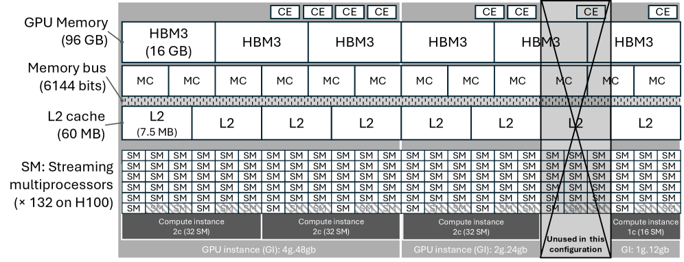</details> Figure 1: Example MIG configuration on a 96 GB H100 GPU. Multi-instance GPU (MIG) [15] is a hardware mechanism which partitions a single GPU into multiple smaller instances. An instance comprises of a portion of the GPU’s compute resources and a portion of the GPU’s memory resources. Each instance is exposed to the user as an independent CUDA device, which is selected using the environment variable CUDA_VISIBLE_DEVICES. In MIG, a GPU instance (GI) represents the combination of a portion of GPU’s compute resources, a portion of memory resources, and a portion of the copy and decoding engines. This resources division is rigid. Both memory and compute resources are allocated as one or multiple slices, with each slice having a fixed size. Each GPU instance gets a fixed number of slices of each type, with a constrained range of possible combinations. A memory slice represents roughly one eighth of the total memory resources, which not only comprises of HBM memory, but also a portion of the L2 cache, a number of the GPU’s copy engines (CE), and dedicated path across the memory controllers. A compute slice represent roughly one seventh of the total compute resources, that is, one seventh of the total SMs count. In reality, the exact SM count significantly deviates from one seventh. Table II lists the available GPU instance profile for a H100 GPU with 132 SMs. The profile name reflects the number of compute and memory slice for each profile. For example, a 3g.24gb profile contains 3 compute slices, that is, roughly 2 sevenths of the total SM count, along with 2 eighths of the total 96 GB GPU memory, that is 24 GB. Once a GPU instance has been created, compute instances must be created on top of it for the resources to be usable to the user. A compute instance represents the top-level MIG instance on which users can execute their application. Figure 1 presents an example MIG configuration for a 96 GB Nvdia H100 GPU. MIG allows to create more than one compute instance atop a single GPU instance. In this case, the compute instances share the memory capacity and L2 cache, but each gets its own set of SMs. This approach is similar to MPS. Compute instances profiles are named by prefixing the name of the underlying GPU instance with the number of compute slices in the compute instance. For example, 2c.3g.48gb designates a compute instance with 2 compute slices (“2c”), on top of a 3g.48gb GPU instance. When the compute instance uses all compute slices of the GPU instance, the first part is omitted: 3c.3g.48gb is abbreviated 3g.48gb. The static configuration in MIG is a known limitation, as changing the MIG configuration is not possible while GPU applications are running. Various solutions have been proposed to tackle this issue, such as dynamic re-configuration [4, 6]. ### II-C Nvlink-C2C Interconnect Nvlink-C2C interconnect was introduced on the Grace Hopper superchip, where CPU and GPU are connected with it to form a cache-coherent “chip-to-chip” interconnect. This high-performance interconnect can deliver up to 450 GB/s bandwidth in each direction. Over Nvlink-C2C, each processor (CPU or GPU) can directly access the other processor’s memory at cacheline granularity, namely 128 bytes on the GPU side, and 64 bytes on the CPU side. Cache-coherency is enforced at the hardware level. When memory is accessed over Nvlink-C2C, the data is transparently cached in the cache hierarchy of the accessing processor. Atomics over Nvlink-C2C are also supported. These features are implemented at the hardware level and do not require any user intervention. ## III Methodology We conduct our experiments on an Nvidia H100 GPU integrated in a Grace Hopper system. This GPU is equipped with 96 GB of HBM3 memory, and features 132 SMs, from the Hopper microarchitecture. Table II presents the various MIG GPU instance profiles available on this device. It is worth noting here that other H100 GPUs, e.g. with different form factors or memory capacities, might have different characteristics for each supported MIG profile [15]. In terms of software, we use CUDA runtime 12.4, Nvidia GPU driver version 550.54.15, and Linux kernel 5.14.0. The CPU is a 72-core Arm Neoverse-V2 CPU, equipped with 512 GB of LPDDR5X memory. TABLE II: A summary of MIG profiles for Grace Hopper H100 (96GB) GPU. Usable resources are given for one MIG instance, wasted resources are GPU-wide best case. Max. SMs Memory (GiB) L2 Mem. BW Profile Inst. Usable Wasted Usable Wasted %GPU Cache CEs (GiB/s) 1g.12gb 7 16 15% 11 17.5 1/8 1/8 1 406 1g.24gb 4 26 21% 23 2.5 2/8 2/8 2 812 2g.24gb 3 32 3% 23 2.5 2/8 2/8 2 812 3g.48gb 2 60 6/9% 46.5 1.5 4/8 4/8 3 1611 4g.48gb 1 64 3% 46.5 1.5 4/8 4/8 4 1635 7g.96gb 1 132 0% 94.5 0 8/8 8/8 8 3175 ### III-A GPU Utilization Metrics To quantify GPU utilization, various approach have been proposed, relying on Nvidia’s system-level monitoring tool: nvidia-smi to monitor memory usage, Nvidia Nsight System to obtain information on SM utilization, and Nvidia Nsight Compute to obtain information on memory bandwidth utilization, and compute throughput for individual kernels [2, 7]. However, these approaches have significant limitations on pre-Hopper GPUs, as bandwidth utilization and compute throughput can only be measured for individual kernels through overhead-inducing profiling, making system-wide monitoring impractical. With the introduction of the Hopper microarchitecture, support for sampling of performance metrics has been added to Nvidia Management Library (NVML), under the name GPU Performance Metrics (GPM). This feature allows sampling GPU performance metrics, either at the GPU level or at the MIG instance level. GPM sampling is exposed to the user in nvidia-smi. However, as this interface provides limited control on the sampling period, we directly use the NVML library to collect GPM metrics. In detail, we collect several GPM metrics, including those associated with the metrics proposed in [2, 7]. We use a sampling period of 0.2 s. First, we collect the SM utilization metric, which reports the percentage of time that SM are busy in the sampling period. In addition, we collect the more granular SM occupancy metrics, which measures the percentage of active warps relative to the hardware maximum over the sampling period. Finally, we collect the pipeline utilization for arithmetic units and Tensor Cores to identify the behavior of each application in an application-agnostic way. Those metrics are reported for each datatype: double-, single-, and half-/mixed-precision. For memory utilization, we collect both capacity usage and bandwidth usage. In addition to GPM metrics, we also capture regular NVML metrics, namely used GPU memory, GPU power draw, GPU clock frequency, and GPU throttling information. For GPU power draw, NVML API support pooling an history of measurements, with a sampling period of 20 ms, other metrics using the same pooling mechanism have a sampling frequency of 200 ms. ### III-B Applications A key aspect for choosing to run an application under MIG is its low scale, and limited memory footprint. For our study we choose a set of application from various domains: high-performance computing, quantum computing, artificial intelligence, and data analytics. In order to evaluate each application under all available MIG profiles, we select problem sizes that fits in GPU memory for the smallest MIG profile on our system, that is, 12 GB. Table III details the selected workloads, and associated data input. The used pipelines column indicates which of the GPU compute pipelines are used by each application, this information is collected through the pipeline utilization metrics in NVML GPM. Collectively, our selection of workloads utilizes all available compute pipelines on Hopper GPU, with the exception of double precision Tensor Cores, which remain unutilized for all evaluated applications. In addition to the set of real-world application, we include two variants of the STREAM benchmark [16]. The STREAM-GPU benchmark executes the STREAM benchmark on the GPU, with data placed locally on the same GPU, this allows us to measure memory bandwidth in MIG. The STREAM-Nvlink variants executes a GPU kernel which reads an array of data placed in CPU memory, and writes back data to another CPU-resident array. This benchmark aims at simulating a heavy load on the CPU-GPU interconnect, in order to evaluate how the Nvlink-C2C link is utilized in MIG, depending on the MIG configuration, and the number of concurrently running applications, on separate MIG instances. For three of the selected applications, namely FAISS, LLama3, and Qiskit, we also decline a problem version above 12 GB. These problem variants are indicated in parenthesis in Table III, and are only used in Section VI. FAISS is an indexing library [17]. The core of the benchmark used in this work queries a vector database using approximate nearest neighbor search. In this context, using an index type with a higher memory footprint can speed up query time or improve accuracy. We therefore swap the index type, yielding an overall higher memory footprint when querying the index. It is worth noting that in this variant, the memory footprint of the application only exceeds GPU memory for a very short amount of time, representing a workload with very short memory usage burst. For the LLM inference benchmark, we use the 8 bit-quantized version (“Q8”) of the Llama3-8B model. This quantization allows executing the model on the smallest MIG profile, at the cost of reduced quality. For the larger test case, we use the original half-precision version of the model, increasing inference quality at the cost of higher memory footprint. For Qiskit, the main data structure is the state vector, consisting of $2^n$ single-precision complex numbers, with $n$ the number of simulated qubits. While a 30-qubit state vector fits within 8 GB of GPU memory, a 31-qubit state vector takes up 16 GB of GPU memory, and is therefore unable to fit within the smallest MIG profile memory. We use the 31-qubit case for our larger test case. For other applications, we do not derive a high-memory variant. AutoDock-GPU does not have a high memory footprint even with large molecule inputs, and therefore does not directly benefit from increasing the GPU memory capacity. NekRS and LAMMPS are codes where the problem to be solved can be user-tuned to fit within given GPU memory. The version of GPT2 training is too limited in scope to exceed the smallest MIG profile memory capacity. TABLE III: A summary of applications. Parenthesis for the input problem indicate a memory footprint above 12 GB. Name Description Used Pipelines Input Qiskit [18] Quantum Simulation FP32 Quantum Volume, 30(-31) qubits FAISS [17] Data analytics FP32, FP16 sift1M IVF4096,PQ64(/IVF16384) NekRS [19] CFD FP64, FP32 turbPipePeriodic LAMMPS [20] Molecular Dynamics FP64 ReaxFF AutoDock-GPU [21] Molecular Docking FP32 PDBID: 3er5, 2vaa LLM Training [22] GPT2 HMMA, FP32 tinystories, shakespeare [23] LLM Inference [24] Llama3 HMMA, IMMA, FP32, FP16 Llama 3 8B Q8 (FP16) [25] Rodinia: hotspot [26] Diff. eq. solver FP64, FP32 1024 $×$ 1024, 1M iterations STREAM-Nvlink Memory Bandwidth FP64 512 MB array STREAM-GPU Memory Bandwidth FP64 512 MB array ### III-C Achievable Resource Utilization in MIG As a first step, we measure precisely the amount of resources allocated for each MIG profile. While the documentation details that a memory slice is approximately one eighth of the total GPU memory, and a compute slice is approximately one seventh of the GPU’s SMs, exact values are not provided. To measure the number of SMs allocated to one MIG instance, we design a benchmark around a simple GPU kernel. The kernel executes a fixed number of arithmetic operations, in a predictable time. The kernel launch configuration is chosen so that one block fully utilizes one streaming multiprocessor for a fixed amount of time, by setting the block size to the maximum admissible number of threads per block (maxThreadsPerBlock). We first launch this kernel with $1$ thread block, measuring the kernel runtime $Δ t$ . We then repeatedly launch the kernel, each time incrementing the thread block count $n$ , measuring the runtime for each execution. The smallest $n$ for which the runtime is $2Δ t$ is such that $n=N_SM+1$ , with $N_SM$ the number of available streaming multiprocessors. This is based on the design of the kernel: when $n$ is equal to the number of streaming multiprocessor, all thread blocks can be scheduled concurrently to run and finish simultaneously after $Δ t$ , with no thread block waiting. Adding one more thread block will result in this block waiting $Δ t$ for the $N_SM$ first blocks to finish before one streaming multiprocessor is freed. We then compare the experimentally-measured streaming multiprocessor count with the number provided by nvidia-smi. In our experiments, those two values matched in all situations. Those values are reported in Table II. Using the measured SM counts, we find that when configured with 1g.12gb profile, only 16 SMs can be used in each instance. Since the system can support seven instances of this profile, it means that 15% SMs ( $7× 16=112$ SMs compared 132 total) cannot be utilized on the GPU. We present the percentage of wasted SMs for each profile in Table II. We note here that this resource waste is due to the limitation of seven GPU instances in MIG. On Ampere A100 GPU, for which MIG was first introduced, this number (7) matches the seven Graphics Processing Clusters (GPC). On Hopper H100 GPUs, the limitation of seven GPU instances remains, even though the number of GPC is eight. In addition, we observe that most MIG configurations leave some memory capacity unused. This is listed as wasted memory in Table II. For example, creating seven MIG 1g.12gb GPU instances will result in 17.5 GiB unused memory capacity. Overall, memory waste is limited compared to SM waste. TABLE IV: Measured Nvlink-C2C bandwidth using cudaMemcpy and direct in-kernel access (GiB/s). | | | | | | Local | Ratio | | --- | --- | --- | --- | --- | --- | --- | | Profile | BOTH | D2H | H2D | Local | % of total bw | D2H/H2D | | 1g.12gb | red!6041.7 | red!6039.6 | red!6044.0 | green!10!yellow!80357.5 | 13% | 0.900 | | 2g.24gb | yellow!8079.2 | red!6039.6 | red!6044.0 | green!20!yellow!80720.5 | 26% | 0.900 | | 3g.24gb | yellow!8079.2 | red!6039.6 | red!6044.0 | green!50!yellow!801383.3 | 50% | 0.900 | | 4g.48gb | yellow!8079.1 | red!6039.6 | red!6044.0 | green!50!yellow!801438.9 | 52% | 0.900 | | 7g.96gb | yellow!8079.2 | red!6039.6 | red!6044.0 | green!80!2732.4 | 100% | 0.900 | | No MIG | green!10!yellow!80329.1 | green!10!yellow!80276.3 | green!10!yellow!80333.1 | green!80!2741.4 | 100% | 0.829 | (a) cudaMemcpy | | | | | | Local | Ratio | | --- | --- | --- | --- | --- | --- | --- | | Profile | BOTH | D2H | H2D | Local | % of total bw | D2H/H2D | | 1g.12gb | red!40!yellow!80282 | yellow!80343 | red!60207 | yellow!80406 | 13% | 1.65 | | 2g.24gb | red!20!yellow!80334 | yellow!80338 | red!30!yellow!80303 | green!20!yellow!80812 | 26% | 1.12 | | 3g.48gb | red!20!yellow!80331 | yellow!80336 | yellow!80348 | green!50!yellow!801611 | 51% | 0.97 | | 4g.48gb | red!20!yellow!80330 | yellow!80338 | yellow!80347 | green!50!yellow!801635 | 51% | 0.97 | | 7g.96gb | red!20!yellow!80327 | yellow!80336 | yellow!80341 | green!80!3175 | 100% | 0.98 | | No MIG | red!20!yellow!80325 | yellow!80336 | yellow!80337 | green!80!3175 | 100% | 1.00 | (b) Direct GPU access ### III-D Nvlink-C2C MIG distributes compute and memory resources across GPU instances, two distinct GPU instances do not compete for memory bandwidth, or compute time. However, the Nvlink-C2C CPU-GPU interconnect is shared between MIG instances, which raises the question of understanding how Nvlink-C2C can be utilized by an application running under MIG. Within GPU applications, we identify two possible approaches to transfer data over Nvlink-C2C between CPU and GPU memory. The first approach relies on calling explicit data movement APIs, such as cudaMemcpy. Those APIs offload data movements to the GPU’s copy engines (CE). As copy engines are distributed across MIG instances, we expect applications using this approach to not interfere with each others when concurrently performing CPU-GPU data movements. However, as one instance only gets a fraction of the GPU’s CEs, the transfer bandwidth over Nvlink-C2C is also limited to a fraction of the overall bandwidth, even if only one MIG instance is performing data transfer. The second approach relies on direct access ability of the GPU’s streaming multiprocessors to access CPU-resident memory directly from within GPU kernels. We design a benchmark to characterize the achievable bandwidth for each of those two approaches. The benchmark performs a copy operation from a source to a destination buffer. By controlling the respective placements of source and destination buffers, we evaluate host-to-device, device-to-host, and local memory bandwidth. For example, host-to-device is obtained by placing source buffer in host (CPU) memory, and destination buffer in device (GPU) memory. Finally, by executing two copy operations in opposite directions in parallel, we measure the bidirectional bandwidth. We derive two variants of this benchmark. The first variant uses a GPU copy kernel to evaluate performance of direct access, inspired by the STREAM benchmark [16]. The second variant uses cudaMemcpy to perform the copy operation, evaluating performance of copy engine-performed data movements. Results for the cudaMemcpy benchmark are presented in Table IV(a). The smallest MIG instance, 1g.12gb, achieves respectively 13% and 14% for H2D and D2H data movements, relative to the Nvlink-C2C bandwidth measured with MIG disabled. As a 1g MIG instance gets one of the eight GPU’s copy engines, these results are expected. However, increasing the MIG instance size does not provide bandwidth improvement, even though more compute engines are advertised for larger MIG instances. This issue is likely a bug, and might get fixed in future driver/runtime versions. Table IV(b) presents the measured direct access bandwidth for each of the MIG profile. For the local memory bandwidth, the achieved bandwidth is also presented as a percentage of the total memory bandwidth, measured with MIG disabled. We observe that this percentage matches the ratio of total memory allocated to each profile, which is consistent with the observation that memory bandwidth is split across MIG instances. We also observe that even for the smallest MIG profile, the direct access benchmark is able to saturate the Nvlink-C2C interconnect in device-to-host direction. This is a key observation, as direct access enable an application running on the smallest MIG instance is able fully utilize the Nvlink-C2C bandwidth, which is not possible with a cudaMemcpy operation. Overall, for any MIG profile, direct GPU access provides the highest bandwidth over Nvlink-C2C, up to 338 GB/s in device-to-host direction, and 348 GB/s in host-to-device direction. However, since this approach relies on a GPU kernel to perform the copy, it cannot be overlapped with computations. ## IV Imbalanced Resource Underutilization In this section, we analyze resource utilization of compute and memory, respectively, when applications running on full GPUs or GPU sharing. We also characterize performance-resource scaling in applications. ### IV-A Compute Resource utilization <details> <summary>2604.08451v1/x2.png Details</summary>  ### Visual Description ## Bar Chart: Average Occupancy Across GPU Configurations and Tasks ### Overview The chart compares average GPU occupancy (y-axis: 0–100%) across 10 computational tasks (x-axis) under four GPU configurations: 1. **7x MIG 1g** (dark green bars) 2. **7x MPS 13%** (green bars) 3. **7x timeslice** (blue bars) 4. **ref: 1 task, full GPU** (blue with diagonal stripes) Tasks include molecular dynamics (e.g., `autodock_2vaa`), machine learning (`llama3`), and scientific simulations (`qiskit_qv_30q`). Occupancy values are approximate, with uncertainty due to visual estimation. --- ### Components/Axes - **X-axis**: Task names (e.g., `autodock_2vaa`, `hotspot`, `qiskit_qv_30q`). - **Y-axis**: Average occupancy (%) from 0% to 100%. - **Legend**: Located at the top, with four entries: - Dark green: 7x MIG 1g - Green: 7x MPS 13% - Blue: 7x timeslice - Blue (diagonal stripes): ref: 1 task, full GPU --- ### Detailed Analysis #### Task-Specific Occupancy (Approximate Values): 1. **autodock_2vaa**: - 7x MIG 1g: ~38% - 7x MPS 13%: ~37% - 7x timeslice: ~22% - ref: 1 task: ~23% 2. **autodock_3er5**: - 7x MIG 1g: ~38% - 7x MPS 13%: ~37% - 7x timeslice: ~21% - ref: 1 task: ~22% 3. **hotspot**: - 7x MIG 1g: ~58% - 7x MPS 13%: ~57% - 7x timeslice: ~60% - ref: 1 task: ~60% 4. **lammps_reaxff**: - 7x MIG 1g: ~40% - 7x MPS 13%: ~39% - 7x timeslice: ~23% - ref: 1 task: ~41% 5. **llama3**: - 7x MIG 1g: ~35% - 7x MPS 13%: ~34% - 7x timeslice: ~24% - ref: 1 task: ~25% 6. **llmc_shakespeare**: - 7x MIG 1g: ~25% - 7x MPS 13%: ~24% - 7x timeslice: ~22% - ref: 1 task: ~23% 7. **llmc_tinystories_bf16**: - 7x MIG 1g: ~40% - 7x MPS 13%: ~39% - 7x timeslice: ~28% - ref: 1 task: ~30% 8. **nekrs_turbpipeperiodic**: - 7x MIG 1g: ~25% - 7x MPS 13%: ~24% - 7x timeslice: ~23% - ref: 1 task: ~14% 9. **faiss_sift1m**: - 7x MIG 1g: ~27% - 7x MPS 13%: ~26% - 7x timeslice: ~10% - ref: 1 task: ~10% 10. **qiskit_qv_30q**: - 7x MIG 1g: ~58% - 7x MPS 13%: ~56% - 7x timeslice: ~62% - ref: 1 task: ~61% --- ### Key Observations 1. **ref: 1 task, full GPU** (striped blue) consistently shows the highest occupancy across most tasks (e.g., `hotspot`, `qiskit_qv_30q`). 2. **7x timeslice** (solid blue) underperforms compared to other configurations in tasks like `faiss_sift1m` (~10% vs. ~27% for 7x MIG 1g). 3. **7x MIG 1g** and **7x MPS 13%** show similar trends, with slight variations (e.g., `llama3`: 35% vs. 34%). 4. **faiss_sift1m** and **nekrs_turbpipeperiodic** exhibit notably low occupancy for all configurations, suggesting these tasks are less GPU-intensive or poorly optimized. --- ### Interpretation The data highlights that **single-task, full GPU utilization** (ref: 1 task) maximizes occupancy for compute-heavy tasks like `hotspot` and `qiskit_qv_30q`, likely due to reduced overhead from task switching. Conversely, **7x timeslice** (multi-tasking) underperforms in tasks with lower computational demands (e.g., `faiss_sift1m`), where context-switching overhead dominates. Tasks like `autodock_2vaa` and `llama3` show balanced performance across configurations, indicating scalability. The disparity in `nekrs_turbpipeperiodic` suggests potential inefficiencies in GPU task allocation or task-specific optimization gaps. This analysis underscores the trade-off between multi-tasking efficiency (7x configurations) and single-task performance, with implications for workload scheduling in GPU-accelerated environments. 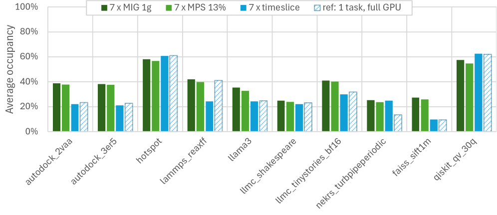</details> Figure 2: GPU compute resource utilization, measured as the SM occupancy using different GPU sharing options. To quantify the compute resources utilization, we measure the average achieved SM occupancy over the entire execution of each workload. Three GPU sharing mechanisms are compared, namely MPS, MIG, and time slice, and the full GPU execution is used for the reference. The results are presented in Figure 2. Streaming Multiprocessor (SM) is the building block of Nvidia GPUs. Each SM can execute instructions independently, and a GPU consists of multiple SMs. At a high level, the number of SMs directly correlates to the compute capacity of a GPU. As shown in Table I, the last four generations of GPUs have not only increased the compute throughput per SM but also packed more SMs in a GPU. If a workload has low SM occupancy, indicating there are not enough active warps to be scheduled to SMs, the peak hardware compute capacity cannot be fully exploited. For workloads that already achieve high SM occupancy in the full GPU execution, GPU sharing may cause their SM occupancy to decrease. For instance, Qiskit, LAMMPS, and hotspot achieve 60%, 40%, and 60% SM occupancy on a full GPU. When running them in the three GPU sharing configurations, their SM occupancy either slightly decreases in MIG and MPS, as in Qiskit and hotspot, or even sharply drops by half in time slicing in LAMMPS. In contrast, if a workload is under-utilizing compute resources in full GPU execution, running in GPU sharing may bring substantial improvement in compute resource utilization. One such example is NekRS, whose SM occupancy is nearly doubled from 12% to 25% in all three GPU sharing configurations. Similarly, the two AutoDock variants have their SM occupancy nearly doubled in GPU sharing. The compute resources underutilization observed at the application level can be explained by two distinct causes at the GPU kernel level. First, as GPU compute resources are increased, kernel execution time on the GPU diminishes. If the shortened GPU execution time is unmatched by a decrease in the CPU execution time, the GPU might become idle. One such case is NekRS, where the CPU-side execution dominates and keeps the GPU idle. The second cause may come from the tail effect in SM scheduling. GPU kernels are divided into thread blocks, which are scheduled onto SMs. Some blocks might finish earlier than others. If no block is available to schedule, some SMs become idle. In the worst case of high imbalance, only one SM remains active while all others are idle. On larger GPUs with more SMs, this tail effect leads to more SMs being left idle compared to smaller GPUs. Such tail effect is observed in the AutoDock workloads. Among the three GPU sharing options, time slicing results in the lowest SM occupancy in most cases, except for hotspot and Qiskit. For instance, AutoDock-3er5 using time-slicing only achieves 20% SM occupancy, while it achieves $38-39$ % SM occupancy in MIG and MPS, nearly a 1.9 $×$ improvement. The high context switch cost in time slicing could be the cause for the overall reduced occupancy. For hotspot and Qiskit, since they have already achieved high SM occupancy in full GPU execution, their lower SM occupancy in GPU sharing could be caused by the wasted SMs (SMs that cannot be scheduled) as explained in Section III-C. MPS always underperforms by 1-5% compared to MIG in all test cases. This could be caused by memory interference, as MPS does not impose any memory isolation. Overall, workloads with low SM utilization can leverage MIG to reduce compute resource underutilization while incurring lower overhead than other options, such as MPS and time slicing. ### IV-B Memory resource utilization <details> <summary>2604.08451v1/x3.png Details</summary>  ### Visual Description ## Bar Chart: Unused GPU Memory by Task and Configuration ### Overview The chart compares unused GPU memory (%) across 10 computational tasks under four GPU configurations: 7x MIG 1g (green), 7x MPS 13% (green with 13% label), 7x timeslice (blue), and a reference configuration of 1 task using the full GPU (striped blue). The y-axis ranges from 0% to 100% unused memory. ### Components/Axes - **X-axis**: Task names (e.g., `autodock_2vaa`, `qiskit_qv_30q`). - **Y-axis**: Unused GPU memory (%) in 20% increments. - **Legend**: - Green: 7x MIG 1g - Green with 13%: 7x MPS 13% - Blue: 7x timeslice - Striped blue: ref: 1 task, full GPU ### Detailed Analysis 1. **autodock_2vaa**: - All configurations show ~95-100% unused memory. - Striped blue (reference) slightly higher (~98%) than others. 2. **autodock_3er5**: - Similar to `autodock_2vaa`, with ~95-100% unused memory. 3. **hotspot**: - 7x MIG 1g and 7x MPS 13%: ~40% unused. - 7x timeslice: ~35%. - Reference: ~90%. 4. **lammps_reaxff**: - 7x MIG 1g and 7x MPS 13%: ~40%. - 7x timeslice: ~35%. - Reference: ~90%. 5. **llama3**: - 7x MIG 1g and 7x MPS 13%: ~40%. - 7x timeslice: ~35%. - Reference: ~90%. 6. **llmc_shakespeare**: - 7x MIG 1g and 7x MPS 13%: ~40%. - 7x timeslice: ~35%. - Reference: ~90%. 7. **llmc_timestories_bf16**: - 7x MIG 1g and 7x MPS 13%: ~65%. - 7x timeslice: ~60%. - Reference: ~90%. 8. **nekrs_turbpipeperiodic**: - 7x MIG 1g and 7x MPS 13%: ~50%. - 7x timeslice: ~45%. - Reference: ~90%. 9. **faiss_sift1m**: - 7x MIG 1g and 7x MPS 13%: ~80%. - 7x timeslice: ~75%. - Reference: ~90%. 10. **qiskit_qv_30q**: - 7x MIG 1g and 7x MPS 13%: ~20%. - 7x timeslice: ~15%. - Reference: ~85%. ### Key Observations - **High Unused Memory**: Tasks like `autodock_*` and `faiss_sift1m` consistently show >80% unused memory across configurations, suggesting low GPU utilization. - **Low Unused Memory**: `qiskit_qv_30q` has the lowest unused memory (~15-20%), indicating high GPU utilization. - **Reference Dominance**: The striped blue (full GPU) configuration consistently shows the highest unused memory (~85-98%), implying inefficiency in resource partitioning for most tasks. - **MPS 13% Underperformance**: The 7x MPS 13% configuration (green with 13%) often performs worse than 7x MIG 1g and 7x timeslice, suggesting potential overhead or suboptimal memory allocation. ### Interpretation The data highlights trade-offs between GPU partitioning strategies: 1. **MIG 1g vs. Timeslice**: Both configurations generally outperform MPS 13% and the full GPU reference, suggesting that partitioning into smaller instances (MIG 1g or timeslice) improves memory efficiency for most tasks. 2. **Task-Specific Behavior**: - Memory-intensive tasks (`autodock_*`, `faiss_sift1m`) benefit less from partitioning, as they leave significant memory unused regardless of configuration. - Compute-heavy tasks (`qiskit_qv_30q`) show minimal unused memory, indicating near-full utilization across all setups. 3. **MPS 13% Inefficiency**: The 7x MPS 13% configuration underperforms in most cases, possibly due to fixed memory allocation constraints or overhead from managing multiple partitions. 4. **Reference as Baseline**: The full GPU configuration (striped blue) serves as a baseline for maximum unused memory, emphasizing that partitioning reduces waste but may not always optimize performance. This analysis underscores the importance of aligning GPU configuration with task requirements to balance memory efficiency and computational throughput. </details> <details> <summary>2604.08451v1/x4.png Details</summary>  ### Visual Description ## BarChart: Average Bandwidth Utilization ### Overview The chart compares average bandwidth utilization across 10 different tasks or applications, measured as percentages. Three configurations are analyzed: - **7x MIG 1g** (green bars) - **7x MPS 13%** (light green bars) - **7x timeslice** (blue bars) A reference line (striped pattern) represents **1 task, full GPU** utilization. ### Components/Axes - **X-axis**: Task/application names (e.g., `autodock_2vaa`, `qiskit_qv_30q`). - **Y-axis**: Average bandwidth utilization (0% to 100%). - **Legend**: - Green: 7x MIG 1g - Light green: 7x MPS 13% - Blue: 7x timeslice - Striped: Reference (1 task, full GPU) ### Detailed Analysis 1. **autodock_2vaa**: - All bars (green, light green, blue) are **<1%**. - Striped reference: **~1%**. 2. **autodock_3ef5**: - All bars (green, light green, blue) are **<1%**. - Striped reference: **~1%**. 3. **hotspot**: - Green: **~5%** - Light green: **~5%** - Blue: **~1%** - Striped reference: **~1%**. 4. **lamms_reaxff**: - Green: **~25%** - Light green: **~25%** - Blue: **~15%** - Striped reference: **~20%**. 5. **llama3**: - Green: **~55%** - Light green: **~50%** - Blue: **~35%** - Striped reference: **~35%**. 6. **llmc_shakespeare**: - Green: **~25%** - Light green: **~25%** - Blue: **~15%** - Striped reference: **~15%**. 7. **llmc_tinystories_bf16**: - Green: **~50%** - Light green: **~50%** - Blue: **~30%** - Striped reference: **~15%**. 8. **neks_turbpipeperiodic**: - Green: **~30%** - Light green: **~35%** - Blue: **~25%** - Striped reference: **~15%**. 9. **faiss_sift1m**: - Green: **~10%** - Light green: **~10%** - Blue: **~5%** - Striped reference: **~5%**. 10. **qiskit_qv_30q**: - Green: **~75%** - Light green: **~80%** - Blue: **~75%** - Striped reference: **~75%**. ### Key Observations - **Highest utilization**: `qiskit_qv_30q` dominates with ~75–80% across all configurations, matching the reference (striped). - **Moderate utilization**: `llama3` and `llmc_tinystories_bf16` show ~50–55% for green/light green, with blue at ~30–35%. - **Low utilization**: `autodock_2vaa`, `autodock_3ef5`, and `hotspot` remain below 5%. - **Striped reference**: Matches the 7x configurations in `qiskit_qv_30q` but is lower for other tasks. ### Interpretation The data suggests that **qiskit_qv_30q** is the most resource-intensive task, utilizing nearly 80% of bandwidth across all configurations. This aligns with the reference (full GPU), indicating it may be a benchmark for maximum utilization. Other tasks like `llama3` and `llmc_tinystories_bf16` show significant utilization but remain below the reference. The **7x MIG 1g** and **7x MPS 13%** configurations generally outperform the **7x timeslice** in most tasks, except for `qiskit_qv_30q`, where all configurations converge. This could imply that the 7x MIG/MPS setups are more efficient for certain workloads, while the timeslice configuration lags behind except in the most demanding case. 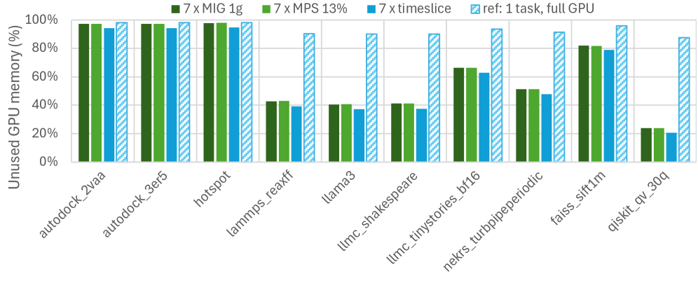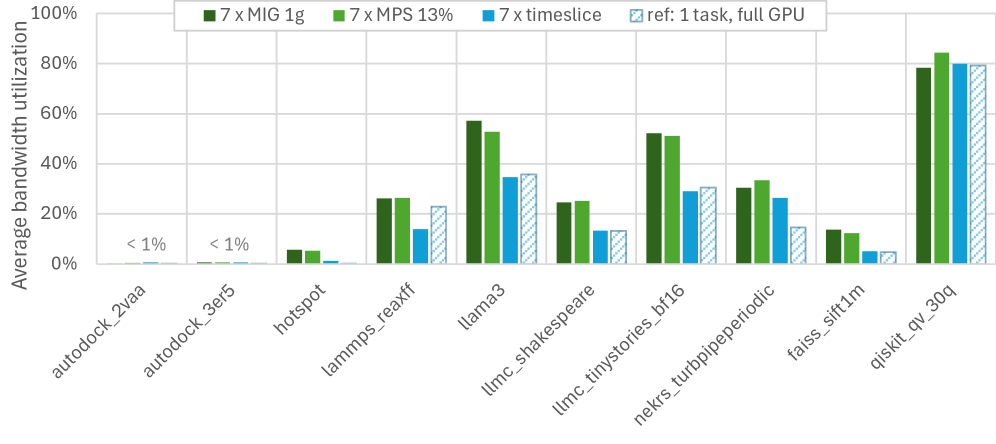</details> Figure 3: GPU memory capacity (upper) and bandwidth (lower) utilization. We analyze memory resource utilization in two aspects, i.e., memory capacity and memory bandwidth. Both aspects directly affect the cost of a GPU system and performance, and thus their utilization needs to be evaluated separately. The memory capacity is often perceived as a hard requirement, as insufficient memory capacity prevents running applications with higher memory needs. On the other hand, bandwidth resource is a more performance-critical requirement, especially for workloads that can efficiently utilize the computing power of GPUs, such as LLM training, whose performance highly depends on memory bandwidth. The top panel of Figure 3 presents the memory capacity underutilization, computed as the used memory relative to total GPU memory, reported by nvidia-smi. As expected, in most cases, using MIG slices significantly reduces unused GPU memory capacity. In fact, seven cases see reduced memory underutilization, by $20$ - $60$ %. AutoDock and hotspot have very low memory footprints and are therefore still significantly underutilizing GPU memory, even with GPU sharing. Memory capacity underutilization arises because the workloads execute with a fixed maximum memory footprint, and do not make use of GPU memory above this footprint. For example, the 8 billion parameters half-precision LLama 3 model fits within 16 GB of memory. This also holds true within a range of scientific applications with fixed problem size, e.g., the AutoDock workloads can fit within 1 GB of GPU memory. We find that time slicing has lower memory waste compared to MIG and MPS. However, since this is a system-level measurement, the memory usage might also include GPU context-induced overhead. To quantify this overhead, we implement a benchmark that initializes a CUDA context without running any computation, allocating memory resources necessary to execute a CUDA application; this is achieved using cudaMalloc(NULL). We measure the memory overhead as $∼$ 60MB per process in MIG 1g.12gb and $∼$ 600MB per process in time slicing. For MPS, we measure a fixed total overhead of $∼$ 600 MB, independent of the number of processes. Clearly, time slicing has the highest GPU context-induced memory overhead, which explains why memory underutilization at system level is lower in time slicing, although the memory is not used by workloads. The bottom panel of Figure 3 presents the memory bandwidth utilization. Only half of the workloads can effectively utilize the memory bandwidth. In these cases, using GPU sharing, as compared to full GPU execution, results in improved bandwidth utilization in all cases, except LAMMPS on time slicing, which has reduced bandwidth utilization. Among the three GPU sharing schemes, time slicing has significantly lower bandwidth utilization, e.g., llama3 achieves 35% utilization in time slicing but 58% in MIG and 52% in MPS. The reduced bandwidth in time slicing is caused by the high context switch overhead, during which no memory operations are performed, reducing the average bandwidth utilization over the entire execution. NekRS and Qiskit achieve higher memory bandwidth utilization in MPS compared to MIG. However, as MPS does not isolate cache between applications, increased memory bandwidth utilization might indicate increased cache conflicts between co-running tasks, generating heavier memory accesses. We identified this to be the case here, as NekRS and Qiskit present degraded performance when co-running under MIG. ### IV-C Coarse-grained Performance-Resource Scaling <details> <summary>2604.08451v1/x5.png Details</summary>  ### Visual Description ## Line Chart: Speedup Over 16 SMS vs. SM Count ### Overview The chart compares the speedup performance of various computational systems (e.g., "hotspot," "qiskit_qv_30q," "llmc_shakespeare") over 16 SMS (Small Molecules) as the SM count increases. The x-axis categorizes SM counts into groups (1g, 2g, 3g(4g), 7g), while the y-axis measures speedup as a multiplier (0–9). A dashed black "ideal" line represents the theoretical maximum speedup. ### Components/Axes - **X-axis (SM count)**: Categorized into 1g, 2g, 3g(4g), 7g. - **Y-axis (Speedup over 16 SMS)**: Linear scale from 0 to 9. - **Legend**: Located on the right, with 10 data series represented by distinct colors and markers: - Blue squares: hotspot - Red circles: qiskit_qv_30q - Purple triangles: llmc_shakespeare - Green diamonds: lammp_reaxff - Pink triangles: llmc_tinystories_bf16 - Orange stars: autodock_2vaa - Brown crosses: autodock_3er5 - Black diamonds: llama3 - Yellow circles: neikrs_turbpipeperiodic - Cyan diamonds: stream_c2c - Dashed black line: ideal ### Detailed Analysis - **1g (16 SMs)**: All lines start near 1.0, with minimal variation. - **2g (32 SMs)**: - hotspot (blue squares) rises to ~2.0. - qiskit_qv_30q (red circles) reaches ~2.2. - stream_c2c (cyan diamonds) remains flat at ~1.2. - **3g(4g) (64 SMs)**: - hotspot peaks at ~4.0. - qiskit_qv_30q reaches ~3.8. - llmc_shakespeare (purple triangles) hits ~3.5. - stream_c2c stays at ~1.2. - **7g (132 SMs)**: - hotspot: ~7.5. - qiskit_qv_30q: ~6.8. - llmc_shakespeare: ~6.5. - lammp_reaxff (green diamonds): ~6.2. - stream_c2c: ~1.2 (flat across all SM counts). ### Key Observations 1. **Ideal vs. Reality**: No system reaches the dashed "ideal" line, which grows linearly from 1.0 to ~8.5 at 7g. 2. **Outliers**: - stream_c2c (cyan diamonds) shows no improvement, remaining at ~1.2. - autodock_2vaa (orange stars) and autodock_3er5 (brown crosses) exhibit slower growth (~2.0–4.5 range). 3. **Trends**: - Most systems show exponential growth, with hotspot and qiskit_qv_30q leading. - llmc_shakespeare and lammp_reaxff follow closely behind. - autodock systems lag, suggesting lower efficiency in scaling. ### Interpretation The chart demonstrates that computational efficiency varies significantly across systems as SM count increases. The "ideal" line represents a linear scaling benchmark, but real-world systems exhibit sublinear or stagnant growth (e.g., stream_c2c). Systems like hotspot and qiskit_qv_30q achieve the highest speedups, suggesting superior optimization for large-scale SM computations. The flat performance of stream_c2c highlights a potential bottleneck or inefficiency in its design. These trends underscore the importance of system-specific optimizations for handling increasing computational loads. </details> Figure 4: GPU Performance-Resource Scaling for each application on a Nvidia Grace Hopper system. 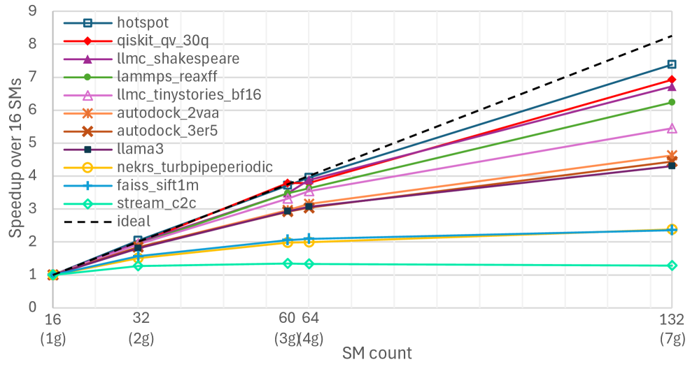From the SM occupancy and memory utilization in previous sections, we find that an application may have imbalanced usage of compute and memory resources. For instance, hotspot has high utilization of compute resources but low memory usage. Qiskit has up to 60% SM occupancy but nearly 90% memory bandwidth usage. In this experiment, we investigate another cause for resource underutilization, i.e., the imbalanced performance scaling as the amount of resources increase. Current resource provisioning via MIG slice is coarse-grained, where GPU compute and memory resources are coupled and increase at nearly a doubling rate. This often mismatches the imbalanced usage of compute and memory resources in real applications. We conduct a performance-resource scaling test, as reported in Figure 4, where each workload runs with increased resources as provisioned with increased MIG slice from 1g.12gb up to 7g.96gb. We report their relative performance by normalizing to the performance obtained in the smallest MIG 1g profile. As the problems in each workload remain constant, with the increased resources, not all workloads scale up their performance proportionally as indicated by the dashed line in Figure 4. Qiskit and hotspot scale the closest to the ideal scaling, with LAMMPS and llmc following a similar scaling. They represent the first category of workloads that have good performance-resource scalability, likely because they achieve balanced high utilization of both compute and memory. The second class of workloads, including AutoDock and llama3 inference, shows a certain deviation from the ideal scaling. Finally, the class of workloads exhibiting the worst scaling is NekRS, FAISS, and STREAM, which heavily utilize memory resources but have limited compute resources. A further investigation indicates that resource underutilization in fixed MIG slices may increase rapidly. This may severely waste resources, especially for the second and third classes of workloads, whose performance-resource scalability is less than ideal. For instance, memory underutilization grows at a higher than doubling rate when increasing the MIG slice. Therefore, the resource requirements of applications scale in a way that mismatches the coarse-grained MIG profiles. There is a need to combine resource underutilization and performance into consideration when selecting suitable GPU sharing options. ## V Opportunities and Challenges in GPU sharing In this section, we analyze opportunities in system-level throughput and energy consumption when GPU sharing is enabled. We also identify power throttling interference as a potential challenge. ### V-A Co-running System Throughput <details> <summary>2604.08451v1/x6.png Details</summary>  ### Visual Description ## Bar Chart: Normalized System Throughput Comparison ### Overview The chart compares normalized system throughput across multiple workloads using different GPU configurations (MIG 7x1g, MIG 7x1c.7g, MPS 7x13%) and a timeslice baseline. A dashed "serial" line at 1.0 serves as a reference point. All values are normalized, with the y-axis ranging from 0 to 3. ### Components/Axes - **X-axis**: Workloads (e.g., `llmc_shakespeare`, `faiss_sift1m`) - **Y-axis**: Normalized system throughput (0–3) - **Legend**: - Dark green: MIG 7x1g - Light green: MIG 7x1c.7g - Blue: MPS 7x13% - Gray (diagonal lines): timeslice - Dashed black line: serial (1.0 baseline) - **Bar Colors**: Match legend entries (e.g., dark green bars = MIG 7x1g) ### Detailed Analysis 1. **Workload Performance**: - **`llmc_shakespeare`**: All configurations cluster near 1.0 (serial baseline). - **`llmc_tinystories_bf16`**: MIG 7x1g (~1.3) and MIG 7x1c.7g (~1.2) outperform MPS 7x13% (~1.1) and timeslice (~0.9). - **`llama3`**: MIG 7x1g (~1.5) and MIG 7x1c.7g (~1.4) exceed MPS 7x13% (~1.3) and timeslice (~1.0). - **`autodock_2vaa`**: MIG 7x1g (~1.5) and MIG 7x1c.7g (~1.4) slightly outperform MPS 7x13% (~1.3) and timeslice (~1.0). - **`autodock_3e5f`**: MIG 7x1g (~1.6) and MIG 7x1c.7g (~1.5) lead over MPS 7x13% (~1.4) and timeslice (~1.1). - **`qiskit_qv_30q`**: MIG 7x1g (~1.0) and MIG 7x1c.7g (~1.1) match MPS 7x13% (~1.0) and timeslice (~0.9). - **`hotspot`**: MIG 7x1g (~0.9) and MIG 7x1c.7g (~0.9) align with MPS 7x13% (~0.9) and timeslice (~0.8). - **`nekrs_turbpipeperiodic`**: MIG 7x1c.7g (~2.6) and MPS 7x13% (~2.7) dominate MIG 7x1g (~2.4) and timeslice (~2.3). - **`lammp_reaxff`**: MIG 7x1g (~1.1) and MIG 7x1c.7g (~1.1) outperform MPS 7x13% (~1.0) and timeslice (~0.6). - **`faiss_sift1m`**: MIG 7x1g (~2.5) and MIG 7x1c.7g (~2.3) lead over MPS 7x13% (~2.3) and timeslice (~1.0). 2. **Trends**: - **MIG 7x1g** (dark green) consistently performs well, often matching or exceeding other configurations. - **MPS 7x13%** (blue) occasionally surpasses MIG 7x1g (e.g., `nekrs_turbpipeperiodic`). - **Timeslice** (gray) is the weakest performer across all workloads. - **Serial baseline** (1.0) is exceeded by all configurations except `llmc_shakespeare`. ### Key Observations - **Outliers**: - `nekrs_turbpipeperiodic` shows the highest throughput (~2.7 for MPS 7x13%). - `lammp_reaxff` has the lowest timeslice performance (~0.6). - **Consistency**: MIG 7x1g and MIG 7x1c.7g configurations generally outperform MPS 7x13% and timeslice. - **Baseline**: The serial line (1.0) acts as a clear performance threshold. ### Interpretation The chart demonstrates that **MIG 7x1g** and **MIG 7x1c.7g** configurations deliver superior throughput compared to MPS 7x13% and timeslice in most workloads. However, **MPS 7x13%** occasionally outperforms MIG 7x1g in specific cases (e.g., `nekrs_turbpipeperiodic`), suggesting workload-dependent optimizations. The **timeslice** configuration consistently underperforms, indicating inefficiencies in its scheduling or resource allocation. The **serial baseline** (1.0) highlights that all tested configurations provide parallel processing advantages, though the degree varies. This data could inform decisions about GPU configuration selection based on workload characteristics. </details> Figure 5: System throughput for concurrent execution of seven workload copies, normalized to serial execution baseline. <details> <summary>2604.08451v1/x7.png Details</summary>  ### Visual Description ## Bar Chart: Normalized Total Energy Across Datasets and Models ### Overview The chart compares normalized total energy consumption across 10 datasets using four computational models: MIG 7x1g, MIG 7x1.7g, MPS 7x13%, and timeslice. A dashed line at 1.0 represents the "serial" baseline. Bars are grouped by dataset, with each model represented by distinct colors (dark green, light green, blue, gray). ### Components/Axes - **X-axis**: Datasets (e.g., `llmc_shakespeare`, `llmc_tinystories_bf16`, `llama3`, `autodock_2vaa`, `autodock_3er5`, `qiskit_qv_30q`, `hotspot`, `neks_turbpipeperiodic`, `lammp_reaxff`, `faiss_sift1m`). - **Y-axis**: "Total energy, normalized" (scale: 0 to 1.5). - **Legend**: - Dark green: MIG 7x1g - Light green: MIG 7x1.7g - Blue: MPS 7x13% - Gray: timeslice - Dashed line: serial (baseline at 1.0). ### Detailed Analysis 1. **Dataset Performance**: - **`llmc_shakespeare`**: Highest energy consumption (~1.2–1.3 for MIG 7x1g and MPS 7x13%). - **`llmc_tinystories_bf16`**: Lowest energy (~0.5–0.6 for all models). - **`hotspot`**: Peaks for MIG 7x1g (~1.2) and MPS 7x13% (~1.3). - **`neks_turbpipeperiodic`**: Lowest values (~0.5–0.6 for all models). - **`lammp_reaxff`**: MIG 7x1g (~0.9) and MPS 7x13% (~1.0) dominate. - **`faiss_sift1m`**: MIG 7x1g (~0.6) and MPS 7x13% (~0.7) show moderate performance. 2. **Model Trends**: - **MIG 7x1g** (dark green): Consistently highest or near-highest values across most datasets. - **MPS 7x13%** (blue): Second-highest performance, often trailing MIG 7x1g. - **MIG 7x1.7g** (light green): Slightly lower than MIG 7x1g but outperforms timeslice. - **timeslice** (gray): Near-baseline performance (~0.8–1.1), slightly above serial in some cases. - **serial** (dashed line): Baseline at 1.0; most models exceed this except in low-energy datasets. ### Key Observations - **Outliers**: - `llmc_shakespeare` and `hotspot` show extreme energy consumption for MIG 7x1g and MPS 7x13%. - `neks_turbpipeperiodic` and `llmc_tinystories_bf16` exhibit uniformly low energy use. - **Trends**: - MIG 7x1g and MPS 7x13% generally outperform other models, suggesting higher computational efficiency. - timeslice performs closer to the serial baseline, indicating minimal parallelization gains in some cases. ### Interpretation The chart demonstrates that MIG 7x1g and MPS 7x13% models achieve the highest normalized energy efficiency across most datasets, with MIG 7x1g leading in high-energy tasks like `llmc_shakespeare` and `hotspot`. The timeslice model shows mixed results, performing near-baseline in low-energy datasets but slightly better in others. The serial baseline (1.0) serves as a reference, highlighting that most models reduce energy consumption compared to sequential processing. Notably, `neks_turbpipeperiodic` and `llmc_tinystories_bf16` require minimal energy across all models, suggesting inherent efficiency in these tasks. The data implies that model choice significantly impacts energy efficiency, with MIG 7x1g being the most resource-intensive but potentially optimal for complex workloads. </details> Figure 6: Total energy consumed for concurrently running 7 GPU-sharing tasks, normalized to the total energy consumed for seven serial runs of the same application. 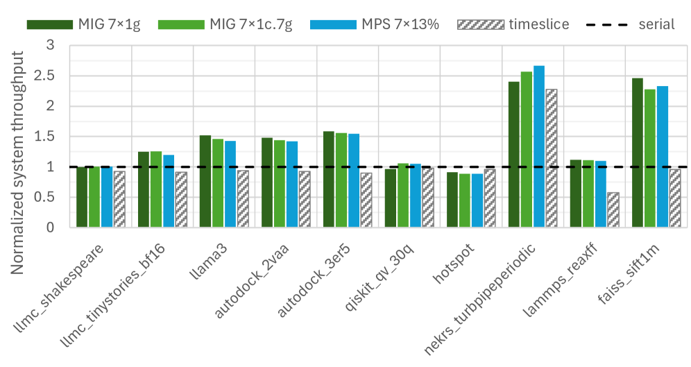We measured aggregated task throughput when running seven instances of an application concurrently across different GPU sharing schemes. Figure 5 shows normalized system throughput, with serial execution as a baseline, obtained by sequentially running seven times the same application on the entire GPU. Overall, running seven applications in parallel on GPU sharing configurations achieves an average throughput improvement of approximately 1.4 $×$ compared to sequential execution, demonstrating the benefit of concurrent execution for system-level efficiency. We measured aggregated task throughput when running seven instances of an application concurrently across different GPU sharing schemes. Figure 5 shows normalized system throughput, where values above 1 indicate improvement over serial execution of the same seven instances. Overall, running seven applications in parallel on GPU sharing configurations achieves an average throughput improvement of approximately 1.4 $×$ compared to sequential execution, demonstrating the benefit of concurrent execution for system-level efficiency. Two applications achieve exceptional throughput gains: NekRS and FAISS reach 2.4 $×$ and 2.5 $×$ improvement with GPU sharing with MIG 7 $×$ 1g respectively. This aligns with their resource utilization characteristics. Both exhibit low GPU compute utilization (13.5% and 10% SM occupancy respectively in Figure 2), substantial unused GPU memory (over 50% as shown in Figure 3), and relatively low bandwidth utilization. Running on smaller MIG instances results in better occupancy and memory utilization, as discussed in Section IV-A, increasing overall system throughput. Conversely, compute-intensive workloads show minimal benefit or slight degradation. Qiskit and hotspot experience less than 5% throughput reduction, consistent with their high compute resource utilization (62% and 61% SM occupancy respectively in Figure 2). Comparing sharing mechanisms, MIG 7 $×$ 1g generally achieves higher throughput than MIG 7 $×$ 1c.7g and MPS 7 $×$ 13%, except for Qiskit and NekRS. These two applications achieve higher memory bandwidth utilization under MPS than MIG (as shown in Figure 3), since because MIG’s strict memory isolation limits each partition to one-seventh of the total bandwidth, while MPS allows more flexible bandwidth sharing. For bandwidth-sensitive workloads, this hardware-enforced isolation in MIG can become a performance bottleneck despite providing better resource guarantees. 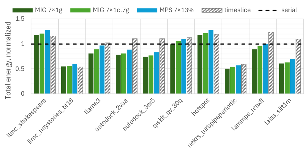### V-B Co-running Energy Utilization To quantify the energy implications of GPU sharing with MIG, we measure total energy consumption for different sharing configurations. The instantaneous GPU-level power consumption is sampled every 20ms using NVML and these measurements are integrated over the total duration to compute total energy. We compared running seven concurrent identical tasks under different GPU sharing configurations against serial execution baseline. Figure 6 shows the normalized results. The results reveal compelling energy efficiency benefits across nearly all workloads tested. GPU sharing demonstrates substantial energy savings in most applications, with reductions ranging from 10% (LAMMPS) variants to over 50% (NekRS). On average, workloads achieve 26% energy reduction compared to serial execution. These savings stem from two primary sources: the elimination of GPU idle periods between sequential task executions, and more efficient amortization of static power consumption across multiple concurrent workloads. However, llmc_shakespeare and hotspot exhibit increased energy consumption under GPU sharing, while Qiskit shows comparable energy to serial execution, suggesting workload-specific sensitivity to sharing mechanisms. Among the four evaluated GPU sharing configurations, MIG 7 $×$ 1g consistently achieves the lowest energy consumption across all benchmarks, on average reducing total energy to 63% of the serial baseline. This fine-grained partitioning approach outperforms MIG 7 $×$ 1c.7g, MPS 7 $×$ 13%, and timeslice scheduling in every workload tested. The efficiency of MIG 7×1g suggests that maximizing parallelism through smaller partitions optimally balances resource utilization with power consumption, providing the most compelling energy efficiency for datacenter deployments where operational costs and environmental impact are critical considerations. 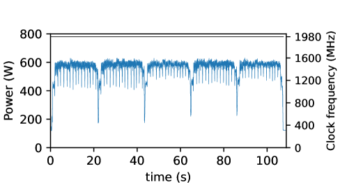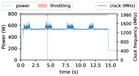#### V-B 1 Power Throttling Interference <details> <summary>2604.08451v1/x8.png Details</summary>  ### Visual Description ## Line Graph: Power and Clock Frequency Over Time ### Overview The image is a line graph depicting the relationship between power consumption, clock frequency, and system throttling over a 15-second interval. Two data series are plotted: power (blue line) and clock frequency (black line), with a pink shaded region indicating throttling periods. The graph includes dual y-axes for power (W) and clock frequency (MHz), with time (s) on the x-axis. --- ### Components/Axes - **X-axis**: Time (s), labeled "time (s)", with ticks at 0.0, 2.5, 5.0, 7.5, 10.0, 12.5, and 15.0 seconds. - **Left Y-axis**: Power (W), labeled "Power (W)", ranging from 0 to 800 W in increments of 200. - **Right Y-axis**: Clock frequency (MHz), labeled "Clock frequency (MHz)", ranging from 0 to 1980 MHz in increments of 400. - **Legend**: Located in the top-left corner, with: - Blue line: "power" - Pink shaded area: "throttling" - Black line: "clock (MHz)" - **Title**: Implied by axis labels and legend; no explicit title text visible. --- ### Detailed Analysis 1. **Power (Blue Line)**: - Starts at 0 W at 0.0s. - Rises sharply to ~700 W by 0.5s. - Fluctuates between ~600–700 W during non-throttling periods. - Drops to ~200 W during throttling periods (pink shading), with sharp vertical declines. - Recovers to ~600–700 W after throttling ends. 2. **Clock Frequency (Black Line)**: - Starts at ~1980 MHz at 0.0s. - Drops to ~400 MHz during throttling periods. - Recovers to ~1980 MHz after throttling ends. - Shows minor fluctuations (~1900–1980 MHz) during non-throttling periods. 3. **Throttling (Pink Shaded Regions)**: - Occurs in four distinct intervals: - 0.5–2.5s - 4.5–6.5s - 8.5–10.5s - 12.5–14.5s - Each throttling period correlates with a drop in both power and clock frequency. --- ### Key Observations - **Inverse Relationship**: Power and clock frequency are inversely correlated during throttling periods. - **Periodic Throttling**: Throttling intervals are evenly spaced (~2.5s apart), suggesting a cyclical or controlled process. - **Sharp Transitions**: Power and clock frequency changes are abrupt during throttling onset/offset, indicating reactive system behavior. - **Recovery Time**: System recovers to baseline power (~700 W) and clock frequency (~1980 MHz) within ~0.5s after throttling ends. --- ### Interpretation This graph illustrates a system undergoing thermal or performance throttling to manage heat or power constraints. The periodic drops in clock frequency and power consumption suggest the system dynamically adjusts its performance to prevent overheating or energy overload. The regularity of throttling intervals implies a programmed or workload-driven trigger (e.g., CPU-intensive tasks followed by cooling periods). The sharp transitions indicate an immediate response mechanism, while the recovery phase reflects the system’s return to normal operation after thermal stabilization. The data highlights the trade-off between performance (clock speed) and efficiency (power consumption) under load management. </details> <details> <summary>2604.08451v1/x9.png Details</summary>  ### Visual Description ## Line Chart: Power and Clock Frequency Over Time ### Overview The image depicts a dual-axis line chart showing two time-series datasets: **Power (W)** and **Clock frequency (MHz)**. The x-axis represents time (0–100 seconds), while the left y-axis (Power) ranges from 0–800 W, and the right y-axis (Clock frequency) ranges from 0–1980 MHz. Two blue lines are plotted: one for Power (left axis) and one for Clock frequency (right axis). --- ### Components/Axes - **X-axis**: Time (s), linear scale from 0 to 100 seconds. - **Left Y-axis**: Power (W), linear scale from 0 to 800 W. - **Right Y-axis**: Clock frequency (MHz), linear scale from 0 to 1980 MHz. - **Lines**: - **Power (W)**: Solid blue line with periodic sharp drops. - **Clock frequency (MHz)**: Dashed blue line with a single sharp drop at the end. --- ### Detailed Analysis 1. **Power (W)**: - Baseline: ~600 W (stable between 0–100 s). - Periodic drops: Occur at ~20, 40, 60, 80, and 100 seconds, with power plummeting to ~200 W before recovering. - Uncertainty: Drops are abrupt (~100 W/sec) but precise in timing. 2. **Clock frequency (MHz)**: - Baseline: ~1600 MHz (stable between 0–95 s). - Final drop: At ~100 seconds, frequency collapses from ~1600 MHz to ~400 MHz. - Uncertainty: Drop is instantaneous (~1200 MHz/sec). --- ### Key Observations - **Periodic Power Drops**: Regular intervals (every ~20 s) suggest cyclical events (e.g., sensor readings, system checks). - **Final Clock Frequency Collapse**: A single catastrophic drop at the end of the timeline, unrelated to earlier Power fluctuations. - **Divergent Behavior**: Power and Clock frequency trends are mostly independent except for the final synchronized drop at 100 s. --- ### Interpretation 1. **Power Drops**: - Likely represent transient events (e.g., voltage regulation, load switching) causing temporary power spikes/drops. The regularity implies a controlled or repetitive process. 2. **Clock Frequency Collapse**: - The abrupt frequency drop at 100 s may indicate a system failure (e.g., thermal shutdown, power loss) or intentional shutdown sequence. Its independence from earlier Power fluctuations suggests a separate failure mode. 3. **System Relationship**: - While Power and Clock frequency are decoupled for most of the timeline, their synchronized drop at 100 s implies a shared dependency on a critical system component (e.g., power supply failure). 4. **Anomalies**: - The Clock frequency drop at 100 s is an outlier compared to its stability earlier. This could signal a boundary condition (e.g., end of test, system reset). --- ### Conclusion The chart reveals a system operating under periodic stress (Power drops) but maintaining stable performance (Clock frequency) until a critical failure at 100 s. The dual-axis visualization highlights the interplay between power management and clock stability, with the final collapse suggesting a systemic vulnerability. </details> (a) Qiskit <details> <summary>2604.08451v1/x10.png Details</summary>  ### Visual Description ## Line Graph: Power and Clock Frequency Over Time ### Overview The image is a line graph depicting two time-series data sets: **power consumption (W)** and **clock frequency (MHz)** over a 15-second interval. A vertical red line marks a "throttling" event at approximately 5.0 seconds. The graph includes a legend, dual y-axes, and a secondary x-axis for time. --- ### Components/Axes - **X-axis (Time)**: Labeled "time (s)" with markers at 0.0, 2.5, 5.0, 7.5, 10.0, 12.5, and 15.0 seconds. - **Left Y-axis (Power)**: Labeled "Power (W)" with values ranging from 0 to 800 W. - **Right Y-axis (Clock Frequency)**: Labeled "Clock frequency (MHz)" with values ranging from 0 to 1980 MHz. - **Legend**: Located in the top-left corner, with: - **Blue line**: "power" - **Red vertical line**: "throttling" - **Black dashed line**: "clock (MHz)" - **Secondary X-axis**: Not explicitly labeled but implied by the time markers. --- ### Detailed Analysis 1. **Power (Blue Line)**: - **Initial Drop**: Power plunges from ~800 W to ~400 W at ~0.5 seconds. - **Stable Phase**: Fluctuates between ~500–700 W from ~0.5s to ~15s, with periodic spikes (e.g., ~600 W at ~2.5s, ~700 W at ~7.5s). - **Final Drop**: Sharp decline to ~200 W at ~15s. 2. **Clock Frequency (Black Dashed Line)**: - **Initial Drop**: Drops from ~1980 MHz to ~1600 MHz at ~0.5 seconds. - **Stable Phase**: Remains near ~1600 MHz until ~15s. - **Final Drop**: Plummets to ~400 MHz at ~15s. 3. **Throttling Marker (Red Vertical Line)**: - Positioned at ~5.0 seconds, coinciding with a power spike (~700 W) and a clock frequency plateau (~1600 MHz). --- ### Key Observations - **Power and Clock Correlation**: Both metrics drop sharply at ~0.5s, suggesting a system response to workload or thermal constraints. - **Throttling Timing**: The throttling marker at 5.0s occurs during a power spike, implying throttling may be triggered by sustained high power. - **Final Drop**: The abrupt decline in both metrics at 15s suggests a system shutdown or critical failure. - **Periodic Spikes**: Power spikes at ~2.5s and ~7.5s may indicate recurring tasks or workload bursts. --- ### Interpretation - **System Behavior**: The graph likely represents a computational workload with dynamic power and clock management. The initial drop at 0.5s could reflect a transition to a lower-power state (e.g., sleep mode), while the throttling at 5.0s indicates thermal or power limits being enforced. - **Anomalies**: The final drop at 15s is abrupt and unexplained by prior trends, possibly signaling a hardware failure or intentional shutdown. - **Throttling Mechanism**: The correlation between power spikes and throttling suggests the system reduces clock frequency to manage thermal/power constraints, though the throttling marker at 5.0s occurs after the initial power drop, raising questions about trigger timing. --- ### Uncertainties - Exact timing of the throttling event (5.0s) may have ±0.1s uncertainty due to visual estimation. - Power spikes (e.g., ~700 W) are approximate, as the graph lacks gridlines for precise interpolation. - The cause of the final drop at 15s is not explicitly stated in the data. 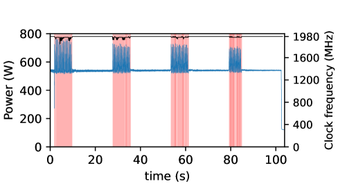</details> <details> <summary>2604.08451v1/x11.png Details</summary>  ### Visual Description ## Dual-Axis Line and Bar Chart: Power Consumption vs. Clock Frequency Over Time ### Overview The chart displays two synchronized datasets over a 100-second interval: 1. **Power consumption** (red bars with blue tops) 2. **Clock frequency** (blue area and black line) The x-axis represents time (0–100 seconds), while the left y-axis shows power in watts (W) and the right y-axis shows clock frequency in megahertz (MHz). A notable feature is the stepwise increase in power and frequency at discrete time intervals, followed by a sharp drop in frequency at the end. --- ### Components/Axes - **X-axis**: Time (s), labeled at 0, 20, 40, 60, 80, 100. - **Left Y-axis (Power)**: 0–800 W, with gridlines every 200 W. - **Right Y-axis (Clock Frequency)**: 0–1980 MHz, with gridlines every 400 MHz. - **Legend**: - **Red**: Power (W) - **Blue**: Clock frequency (MHz) - **Key Elements**: - Vertical red bars with blue tops (power spikes). - Black stepwise line (clock frequency trend). - Blue shaded area (constant frequency during intervals). --- ### Detailed Analysis 1. **Power (Red Bars)**: - Five vertical red bars appear at **0, 20, 40, 60, and 80 seconds**. - Each bar’s base is ~500 W, with blue tops reaching **~600–800 W** (uncertainty: ±50 W). - The black line atop the bars shows a stepwise increase, peaking at **~800 W** at 80 seconds. 2. **Clock Frequency (Blue Area/Line)**: - A flat blue line at **~1600 MHz** spans the entire x-axis, except for a sharp drop at **80 seconds**. - Post-80 seconds, frequency plunges to **~400 MHz** (uncertainty: ±50 MHz). 3. **Blue Shaded Area**: - Covers the region between red bars, indicating sustained clock frequency during active intervals. --- ### Key Observations - **Stepwise Power/Frequency Increases**: Power and frequency rise abruptly at each 20-second interval, suggesting periodic operational bursts. - **Sudden Frequency Drop**: At 80 seconds, clock frequency drops by **~1200 MHz** (from 1600 MHz to 400 MHz), possibly indicating a shutdown or low-power mode. - **Power Consistency**: Power remains stable (~600 W) during active intervals but aligns with the black line’s stepwise trend. --- ### Interpretation - **Operational Cycles**: The chart likely represents a system (e.g., CPU, GPU) executing periodic high-power tasks. The stepwise increases in power and frequency suggest scheduled workloads or clock speed adjustments. - **Power Management**: The abrupt frequency drop at 80 seconds implies a transition to a low-power state, possibly after task completion or user inactivity. - **Data Gaps**: No data is recorded between 80 and 100 seconds for power, but the frequency remains at 400 MHz. This could indicate idle mode or measurement cessation. The chart highlights a correlation between power consumption and clock frequency during active periods, with a clear emphasis on energy efficiency post-80 seconds. </details> (b) LLM training Figure 7: Power consumption and throttling behavior for (a) Qiskit and (b) LLM training. Left: single application on full GPU. Right: concurrent executions on 7 $×$ 1g MIG partitions. Pink regions indicate power throttling periods. By monitoring GPU power draw and clock frequencies at 20ms intervals during concurrent execution, we observe power throttling behavior. Figure 7 shows representative power traces for memory-bound (Qiskit) and compute-intensive (LLM training) workloads under both isolated (left) and concurrent (right) execution scenarios. Memory-bound workloads experience reduced power consumption under GPU sharing. Qiskit running on the full GPU (Figure 7(a), left) exhibits continuous throttling, hitting the 700W power limit and dropping clock frequencies from 1980 MHz down to 1815 MHz. When seven instances of Qiskit execute in parallel, each on its 1g.12gb MIG instance (Figure 7(a), right), we observe a maximum power consumption of 670W, below the 700W power cap. Therefore, no throttling is observed. The MIG bandwidth partitioning naturally constrains power draw below throttling thresholds, eliminating throttling but reducing per-instance performance. Compute-intensive workloads trigger power throttling only during concurrent execution. LLM training running alone (Figure 7(b), left) maintains 500-650 W power consumption without throttling. However, seven concurrent instances on independent MIG 1g instances (Figure 7(b), right) collectively exceed the 700 W limit, causing periodic throttling with associated frequency drop. This occurs despite performance isolation promises in MIG, as hardware partitioning isolates compute and memory resources but not power delivery. Above observations reveal a potential challenge in GPU sharing: while MIG provides logical resource isolation, shared power delivery creates a side channel for interference. ## VI GPU Sharing with Nvlink-C2C enabled Offloading ### VI-A Nvlink-C2C Offloading The characteristics of MIG instances are fixed, and the choice of a MIG profile is limited to a fixed set of possible memory capacities, that are multiples of the smallest memory slice, namely 12 GB on our platform. When a workload’s memory footprint is slightly above the memory capacity of a given MIG profile, the next larger profile must be used to enable execution of the workload. Such choice comes with a significant increase in memory capacity, even though the workload to execute might only utilize a fraction of this added memory capacity. Taking the example of Qiskit, a 31-qubit simulation consumes 16 GB of GPU memory, that is, 4 GB more than the smallest 12 GB MIG profile. However, running such workload requires selecting a 24 GB MIG profile, leaving 8 GB of memory unused, that is 33% of the GPU instance memory. For such workloads, instead of increasing the MIG instance size, we propose to offload part of the application’s data to host (CPU) memory. During GPU computations, part of the data is accessed over Nvlink-C2C. We implement such offloading strategy for three of the applications, as described in Section III, namely FAISS, Qiskit, and Llama3. We implement the offloading scheme in FAISS and Llama3 by using a memory allocator that supports spilling out of GPU memory, namely cudaMallocManaged or malloc, focusing on performing this change on the large data structures used by each application. For FAISS this is the index data, and for Llama3, we change the allocator used in the GGML backend. We try a similar implementation in Qiskit. However, the natively-supported memory swapping strategy used by Qiskit to spill the state vector over GPU memory appeared to consistently outperform our implementation, we therefore use this swapping strategy to serve the purpose of offloading part of the application’s data to host memory. ### VI-B Reward Model The offloading scheme is expected to increase resource utilization. In Section IV-C we detail how, for a given application, SM occupancy tends to increase as the instance size is reduced. Therefore, our offloading scheme is expected to enable increasing the SM occupancy due to the reduced MIG instance size. In addition, the offloading scheme reduces the unused GPU memory. However, data access over Nvlink-C2C comes with a significant performance cost, an application executing with our offloading scheme might therefore suffer significant performance degradation. To quantify the tradeoff between application performance and resource utilization, we design a simple parametrized cost-benefit model. For this purpose, we consider a MIG instance with a memory capacity ${M}_instance$ and $N_SM$ streaming multiprocessors. We execute the application under study on this MIG instance, measuring the application performance $P$ , the average occupancy at the GPU level ${Occ}$ , and the peak memory usage $M_app$ . By normalizing the occupancy to the MIG instance, based on the total number of SM on the GPU $N_SM,GPU$ , we define the SM waste, noted $W_SM$ . Analogously, we define the memory waste, $W_MEM$ : $$ \begin{cases}W_SM=\frac{N_SM}{N_SM,GPU}(1-Occ)\vskip 2.84544pt\\ W_MEM=\frac{M_instance-M_app}{M_GPU}\end{cases} $$ We measure the application performance $P_GPU$ , obtained when running the application on the entire GPU. From the SM waste, the memory waste, the relative performance $P/P_GPU$ , and a dimensionless term $α$ we derive the following cost-benefit model: $$ R=\frac{P/P_GPU}{α+W_MEM+W_SM} $$ For a fixed application and a fixed value of $α$ , we aim at finding the MIG configuration that maximizes $R$ . The term $α$ represents a policy used to establish whether the model should prioritize reducing resource underutilization ( $α=0$ ), or to prioritize increasing performance, by setting a positive value for $α$ . As $α$ is increased above 0, the model shifts from a utilization-only model to a performance-only model. Since both $W_SM$ and $W_MEM$ are within $[0,1]$ , we vary $α$ within the same range, to ensure it operates on a comparable scale. Increasing $α$ beyond $1$ this range would further favor performance at the cost of greater resource underutilization. ### VI-C Results We apply our model to the three selected applications. For Qiskit and FAISS, we define the performance metric $P$ as the inverse of the runtime. For Llama3, the performance $P$ is the number of token generated per second during the text generation phase of the benchmark. Higher value of $P$ indicates higher performance. Figure 8 presents the reward value produced by our model for a set of MIG configurations for three different applications, with different policies $α$ . The results when using the proposed offloading scheme is also presented, with a MIG instance size of 1g.12gb. Looking at the first row, with $α=0$ , that is, we prioritize reducing resource waste, without penalizing low performance. With this choice, the offloading scheme yields the highest reward for both FAISS and Llama3. However, for Qiskit, the most favored configuration for $α=0$ is 2g.24gb. This is because in this application, the occupancy is the highest for the 2g.24gb case, making this case the best from the perspective of reducing resource underutilization. When increasing $α$ to $0.1$ , the offloading scheme is only preferred for the FAISS case. We suggest that this is because FAISS offloads a small fraction of the overall application working set to host memory, for a very short period of time, resulting in limited performance degradation. Therefore, when including performance to a limited extent in our model ( $α>0$ ), the offloading configuration is still preferred. Setting $α$ to $1$ shifts the preference towards MIG instances with larger sizes, which is expected as this variant of the model prioritizes performance over reducing underutilization. For Llama3 and Qiskit, the largest configuration, namely full GPU, is preferred. This is expected, as discussed in Section IV-C, those two workload, exhibit a near-perfect performance scaling behavior as the number of streaming multiprocessor is increased. In contrast, for FAISS, our model indicates a preference for the 2g.24gb configuration. This is because this particular test case exhibits poor scaling behavior when increasing MIG size, as discussed in Section IV-C. <details> <summary>2604.08451v1/x12.png Details</summary>  ### Visual Description Icon/Small Image (897x32) </details> <details> <summary>2604.08451v1/x13.png Details</summary>  ### Visual Description ## Bar Charts: Reward Distribution Across Conditions (α=0) ### Overview The image contains three grouped bar charts comparing reward distributions across four categories ("High", "Medium", "Low", "None") under a shared parameter α=0. Each chart uses a color-coded legend to distinguish conditions, with bars representing reward magnitudes. The y-axis scales vary between charts (0–4, 0–6, 0–8), suggesting different experimental contexts or normalization methods. ### Components/Axes - **X-axis**: Categories labeled "High", "Medium", "Low", "None" (left to right). - **Y-axis**: "reward" with discrete integer values (0–8 in increments of 2). - **Legend**: Positioned right of all charts, associating: - Dark green: Condition A - Medium green: Condition B - Light green: Condition C - **Chart Labels**: All three charts explicitly marked with α=0. ### Detailed Analysis 1. **Left Chart (α=0)**: - **High**: ~3.8 (dark green, tallest bar) - **Medium**: ~2.5 (medium green) - **Low**: ~2.0 (light green) - **None**: ~1.0 (lightest green) - **Trend**: Reward decreases monotonically from "High" to "None". 2. **Middle Chart (α=0)**: - **High**: ~4.0 (dark green, tallest) - **Medium**: ~2.2 (medium green) - **Low**: ~2.1 (light green) - **None**: ~0.5 (lightest green) - **Trend**: Sharp drop from "High" to "Medium", then slight decrease to "None". 3. **Right Chart (α=0)**: - **High**: ~1.5 (dark green) - **Medium**: ~3.0 (medium green) - **Low**: ~2.5 (light green) - **None**: ~6.0 (lightest green, tallest bar) - **Trend**: "None" category exhibits an anomalous spike (~6.0), exceeding all other conditions. ### Key Observations - The "None" category shows extreme variability: ~1.0 (left), ~0.5 (middle), and ~6.0 (right). - The right chart’s "None" reward (~6.0) is an outlier, surpassing all other conditions by 2–4x. - Dark green ("High") consistently has the highest rewards in left/middle charts but is lowest in the right chart. ### Interpretation The data suggests α=0 modulates reward distributions differently across conditions. The right chart’s "None" category anomaly (~6.0) may indicate: 1. A data collection error (e.g., mislabeled category). 2. A contextual factor unique to that chart (e.g., experimental setup). 3. A non-linear relationship between α and reward when "None" is present. The legend’s color coding implies conditions A–C are systematically varied, but without explicit labels, their exact meaning remains ambiguous. The y-axis scaling differences (0–4 vs. 0–8) complicate direct comparisons between charts, suggesting they may represent distinct experimental phases or normalization techniques. </details> <details> <summary>2604.08451v1/x14.png Details</summary>  ### Visual Description ## Bar Chart: Reward Distribution Across Alpha Values (α = 0.1, 0.3, 0.5) ### Overview The image displays three grouped bar charts comparing reward distributions across six categories (0–5) for three distinct alpha (α) values: 0.1, 0.3, and 0.5. Each chart uses varying shades of green to represent different α values, with darker greens corresponding to higher α. The y-axis measures "reward" (0–2), and the x-axis represents categorical groups (0–5). --- ### Components/Axes - **Y-Axis**: Labeled "reward" with a scale from 0 to 2 in increments of 0.5. - **X-Axis**: Labeled with categories 0–5. - **Legend**: Located on the right, mapping: - Dark green → α = 0.5 - Medium green → α = 0.3 - Light green → α = 0.1 - **Charts**: Three side-by-side bar charts, each corresponding to one α value. --- ### Detailed Analysis #### Chart 1 (α = 0.1) - **Category 0**: Light green bar (~0.6) - **Category 1**: Medium green bar (~1.0) - **Category 2**: Dark green bar (~1.2) - **Category 3**: Medium green bar (~0.8) - **Category 4**: Light green bar (~0.5) - **Category 5**: Medium green bar (~0.7) #### Chart 2 (α = 0.3) - **Category 0**: Medium green bar (~1.1) - **Category 1**: Dark green bar (~1.3) - **Category 2**: Light green bar (~0.9) - **Category 3**: Medium green bar (~1.0) - **Category 4**: Dark green bar (~1.4) - **Category 5**: Light green bar (~0.6) #### Chart 3 (α = 0.5) - **Category 0**: Light green bar (~0.5) - **Category 1**: Medium green bar (~0.8) - **Category 2**: Dark green bar (~1.1) - **Category 3**: Medium green bar (~1.0) - **Category 4**: Light green bar (~0.7) - **Category 5**: Dark green bar (~1.8) --- ### Key Observations 1. **α = 0.5 (Darkest Green)**: - Highest reward in **Category 5** (~1.8), significantly taller than other categories. - Lowest reward in **Category 0** (~0.5), suggesting a potential trade-off between exploration (lower α) and exploitation (higher α). 2. **α = 0.3 (Medium Green)**: - Most balanced distribution, with **Category 4** having the highest reward (~1.4). - No extreme outliers compared to other α values. 3. **α = 0.1 (Lightest Green)**: - Most uniform distribution, with rewards clustering between ~0.5 and ~1.2. - **Category 2** has the highest reward (~1.2), while **Category 4** is the lowest (~0.5). 4. **Trend Across α Values**: - Higher α (darker green) generally correlates with higher rewards in **Categories 2, 4, and 5**. - Lower α (lighter green) shows more uniform rewards but lower peaks. --- ### Interpretation The data suggests that increasing α (likely representing a parameter like exploration-exploitation trade-off in reinforcement learning) amplifies rewards in specific categories (e.g., Category 5 at α = 0.5). However, this comes at the cost of reduced rewards in others (e.g., Category 0 at α = 0.5). The uniformity of rewards at lower α (0.1) implies a more exploratory strategy, while higher α values prioritize exploitation, leading to polarized outcomes. The stark difference in Category 5’s reward (~1.8 at α = 0.5 vs. ~0.7 at α = 0.1) highlights α’s critical role in shaping decision-making dynamics. Anomalies, such as Category 0’s consistent underperformance at higher α, may indicate systemic limitations in the model’s ability to generalize across all categories. </details> <details> <summary>2604.08451v1/x15.png Details</summary>  ### Visual Description ## Bar Chart: Reward Comparison Across Methods (α = 0.5) ### Overview The image contains three horizontally aligned bar charts comparing reward values across five categories: "Baseline," "Method A," "Method B," "Method C," and "Method D." Each chart shares identical axis labels and legend but displays distinct reward distributions. The y-axis ranges from 0 to 1, while the x-axis lists the five categories. All bars use green shades, with a legend on the right mapping colors to methods. ### Components/Axes - **Y-Axis**: Labeled "reward" with a scale from 0 to 1 in increments of 0.2. - **X-Axis**: Categories: "Baseline," "Method A," "Method B," "Method C," "Method D." - **Legend**: Located on the right, with color-coded labels: - Dark green: Baseline - Medium green: Method A - Light green: Method B - Pale green: Method C - Very light green: Method D ### Detailed Analysis #### Chart 1 (Leftmost) - **Baseline**: ~0.2 (dark green) - **Method A**: ~0.35 (medium green) - **Method B**: ~0.45 (light green) - **Method C**: ~0.55 (pale green) - **Method D**: ~0.6 (very light green) - **Trend**: Steady upward progression from Baseline to Method D. #### Chart 2 (Middle) - **Baseline**: ~0.7 (dark green) - **Method A**: ~0.75 (medium green) - **Method B**: ~0.9 (light green) - **Method C**: ~0.7 (pale green) - **Method D**: ~0.4 (very light green) - **Trend**: Peak at Method B, followed by a sharp decline for Method D. #### Chart 3 (Rightmost) - **Baseline**: ~0.15 (dark green) - **Method A**: ~0.25 (medium green) - **Method B**: ~0.45 (light green) - **Method C**: ~0.55 (pale green) - **Method D**: ~0.65 (very light green) - **Trend**: Gradual increase across all methods, with Method D highest. ### Key Observations 1. **Consistency**: Method D consistently achieves the highest reward in Charts 1 and 3 but underperforms in Chart 2. 2. **Outlier**: In Chart 2, Method B surpasses all others, while Method D drops to the lowest value. 3. **Baseline Variability**: Baseline values range from ~0.15 to ~0.7 across charts, suggesting differing starting conditions. ### Interpretation The charts illustrate how reward distributions vary across methods under a fixed parameter (α = 0.5). Method D generally performs robustly, except in Chart 2, where its reward plummets despite others remaining stable. This anomaly could indicate sensitivity to α or method-specific interactions. The Baseline's wide range suggests contextual factors (e.g., data quality, initialization) significantly influence outcomes. Method B's dominance in Chart 2 highlights potential situational advantages, warranting further investigation into its design or training conditions. The consistent upward trend in Charts 1 and 3 implies incremental improvements with newer methods, though diminishing returns are evident in Chart 2's sharp decline for Method D. </details> <details> <summary>2604.08451v1/x16.png Details</summary>  ### Visual Description ## Bar Chart: Reward Distribution Across Categories for α=1 ### Overview The image contains three vertically aligned bar charts labeled "α=1" on the left. Each chart displays three bars in dark green, medium green, and light green, representing reward values on a y-axis (0–0.6). The x-axis is divided into three categories labeled A, B, and C. A legend on the right associates colors with categories: dark green = A, medium green = B, light green = C. All charts share identical axis labels and scales. ### Components/Axes - **Y-axis**: "reward" (0 to 0.6 in increments of 0.2). - **X-axis**: Categories A, B, C (no numerical labels). - **Legend**: Right-aligned, mapping colors to categories (dark green = A, medium green = B, light green = C). - **Title**: Implicitly labeled "α=1" for all charts. ### Detailed Analysis 1. **Chart 1 (Left)**: - **Dark green (A)**: ~0.1 - **Medium green (B)**: ~0.25 - **Light green (C)**: ~0.4 - **Trend**: Reward increases from A to C. 2. **Chart 2 (Center)**: - **Dark green (A)**: ~0.4 - **Medium green (B)**: ~0.5 - **Light green (C)**: ~0.55 - **Trend**: Reward increases from A to C, with the highest value in C. 3. **Chart 3 (Right)**: - **Dark green (A)**: ~0.1 - **Medium green (B)**: ~0.2 - **Light green (C)**: ~0.5 - **Trend**: Reward increases from A to C, with the largest gap between B and C. ### Key Observations - **Consistent Color-Category Mapping**: Dark green (A), medium green (B), light green (C) across all charts. - **Reward Magnitude**: Chart 2 has the highest rewards overall (~0.55), while Chart 1 has the lowest (~0.4). - **Category C Dominance**: Light green (C) consistently shows the highest reward in all charts, with the largest absolute increase in Chart 3 (~0.3 from B to C). ### Interpretation The data suggests that under the condition α=1, category C (light green) consistently yields the highest reward across all scenarios. The variation in reward magnitudes between charts implies differences in experimental conditions or parameters (e.g., environmental factors, system configurations) that amplify rewards for category C. The steepest increase in Chart 3 highlights a potential nonlinear relationship between α and reward distribution, though α is fixed at 1 here. The uniformity of color-coding reinforces the reliability of categorical comparisons, while the absence of error bars or confidence intervals limits conclusions about statistical significance. </details> <details> <summary>2604.08451v1/x17.png Details</summary>  ### Visual Description Icon/Small Image (996x31) </details> Figure 8: Reward based selection ( $α=0,0.1,0.5,1$ ) in three applications. ## VII Related Works Characterization of GPU sharing techniques have previously been conducted. Gilman et al. [12] compare priority streams, time-slicing and MPS. For MPS, Xu et al. [27] quantify interference risk by measuring L2 cache misses. Architectural and software changes have also been proposed to improve multi-application concurrency [28, 29, 9]. Li et al [5] provides an evaluation of MIG performance and energy consumption for machine learning workloads. Works tend to demonstrate a reduced interference risk compared to MPS [4, 30]. While existing works focus on a single range of workload, notably deep learning, we instead offer an application-agnostic approach, covering a broad scope of workloads spanning scientific computing, AI, and data analytics. Existing works on MIG have focused on mitigating impact of co-locating workloads on GPUs at the scheduler level. Tan et al. [11] propose an approach to identify optimal MIG partitioning for DNN model serving. MIG has also been considered at the cluster level for LLM model serving [31, 32]. Combined use of MPS and MIG have also been proposed; either by using measured MPS performance to execution with MIG [4], or by using MPS atop MIG for execution [30]. Our work identifies GPU resource underutilization issues, and propose a cost-benefit model to evaluate the trade-off between performance and resource utilization across MIG configurations. Memory offloading to CPU memory has been proposed as a solution to overcome GPU memory limitations. Studies of this approach over Nvlink-C2C have been conducted [33, 34]. We use memory offloading as a solution to reduce resource underutilization, caused by the rigidity of MIG configurations. ## VIII Conclusion This work provides a first in-depth exploration of using GPU sharing to tame resource underutilization in HPC applications, including real-world scientific, LLM, and data analytics applications. We propose multiple metrics to quantify compute and memory resource underutilization, respectively. Our results indicate that the coarse-grained resource scaling of tightly coupled compute and memory resources, as provided in MIG slices, mismatches the resource-performance scaling characteristics of applications. To address the discontinuity in resource provisioning due to fixed MIG profiles, we leverage Nvlink-C2C offloading to enable workloads slightly larger than a MIG slice to run without requesting a larger MIG profile. Moreover, we propose a new reward metric to trade off the system-level throughput and resource underutilization, and evaluated different choices of GPU sharing in eight workloads using the reward metric on a Grace Hopper system. ## Acknowledgments This research is supported by the Swedish Research Council (no. 2022.03062). This work has received funding from the European High Performance Computing Joint Undertaking (JU) and Sweden, Finland, Germany, Greece, France, Slovenia, Spain, and the Czech Republic under grant agreement No. 101093261. ## References - [1] M. Han, H. Zhang, R. Chen, and H. Chen, “Microsecond-scale preemption for concurrent GPU-accelerated DNN inferences,” in 16th USENIX Symposium on Operating Systems Design and Implementation (OSDI 22), 2022, pp. 539–558. - [2] F. Strati, X. Ma, and A. Klimovic, “Orion: Interference-aware, fine-grained gpu sharing for ml applications,” in Proceedings of the Nineteenth European Conference on Computer Systems, 2024, pp. 1075–1092. - [3] C. Gregg, J. Dorn, K. Hazelwood, and K. Skadron, “Fine-Grained resource sharing for concurrent GPGPU kernels,” in 4th USENIX Workshop on Hot Topics in Parallelism (HotPar 12), 2012. - [4] B. Li, T. Patel, S. Samsi, V. Gadepally, and D. Tiwari, “Miso: exploiting multi-instance gpu capability on multi-tenant gpu clusters,” in Proceedings of the 13th Symposium on Cloud Computing, 2022, pp. 173–189. - [5] B. Li, V. Gadepally, S. Samsi, and D. Tiwari, “Characterizing multi-instance GPU for machine learning workloads,” in 2022 IEEE International Parallel and Distributed Processing Symposium Workshops (IPDPSW). IEEE, 2022, pp. 724–731. - [6] B. Wu, Z. Zhang, Z. Bai, X. Liu, and X. Jin, “Transparent $\{$ GPU $\}$ sharing in container clouds for deep learning workloads,” in 20th USENIX Symposium on Networked Systems Design and Implementation (NSDI 23), 2023, pp. 69–85. - [7] A. Weaver, K. Kavi, D. Milojicic, R. P. H. Enriquez, N. Hogade, A. Mishra, and G. Mehta, “Granularity-and interference-aware gpu sharing with mps,” in SC24-W: Workshops of the International Conference for High Performance Computing, Networking, Storage and Analysis. IEEE, 2024, pp. 1630–1637. - [8] Nvidia, “Nvidia multi-process service overview (r575),” 2025. - [9] M. Pavlidakis, G. Vasiliadis, S. Mavridis, A. Argyros, A. Chazapis, and A. Bilas, “Guardian: Safe gpu sharing in multi-tenant environments,” in Proceedings of the 25th International Middleware Conference, 2024, pp. 313–326. - [10] X. Shi, C. Cai, J. Du, Z. Zhu, and Z. Jia, “Nexus: Taming throughput-latency tradeoff in llm serving via efficient gpu sharing,” arXiv e-prints, pp. arXiv–2507, 2025. - [11] C. Tan, Z. Li, J. Zhang, Y. Cao, S. Qi, Z. Liu, Y. Zhu, and C. Guo, “Serving dnn models with multi-instance gpus: A case of the reconfigurable machine scheduling problem,” arXiv preprint arXiv:2109.11067, 2021. - [12] G. Gilman and R. J. Walls, “Characterizing concurrency mechanisms for nvidia gpus under deep learning workloads,” ACM SIGMETRICS Performance Evaluation Review, vol. 49, no. 3, pp. 32–34, 2022. - [13] Nvidia, “Cuda runtime api documentation,” 2025. - [14] ——, “Cuda driver api documentation,” 2025. - [15] ——, “Nvidia multi-instance gpu user guide,” 2024. - [16] J. D. McCalpin, “Memory bandwidth and machine balance in current high performance computers,” IEEE Computer Society Technical Committee on Computer Architecture (TCCA) Newsletter, pp. 19–25, Dec. 1995. - [17] M. Douze, A. Guzhva, C. Deng, J. Johnson, G. Szilvasy, P.-E. Mazaré, M. Lomeli, L. Hosseini, and H. Jégou, “The faiss library,” arXiv preprint arXiv:2401.08281, 2024. - [18] A. Javadi-Abhari, M. Treinish, K. Krsulich, C. J. Wood, J. Lishman, J. Gacon, S. Martiel, P. D. Nation, L. S. Bishop, A. W. Cross et al., “Quantum computing with qiskit,” arXiv preprint arXiv:2405.08810, 2024. - [19] P. Fischer, S. Kerkemeier, M. Min, Y.-H. Lan, M. Phillips, T. Rathnayake, E. Merzari, A. Tomboulides, A. Karakus, N. Chalmers et al., “Nekrs, a gpu-accelerated spectral element navier–stokes solver,” Parallel Computing, vol. 114, p. 102982, 2022. - [20] A. P. Thompson, H. M. Aktulga, R. Berger, D. S. Bolintineanu, W. M. Brown, P. S. Crozier, P. J. In’t Veld, A. Kohlmeyer, S. G. Moore, T. D. Nguyen et al., “Lammps-a flexible simulation tool for particle-based materials modeling at the atomic, meso, and continuum scales,” Computer physics communications, vol. 271, p. 108171, 2022. - [21] D. Santos-Martins, L. Solis-Vasquez, A. F. Tillack, M. F. Sanner, A. Koch, and S. Forli, “Accelerating autodock4 with gpus and gradient-based local search,” Journal of chemical theory and computation, vol. 17, no. 2, pp. 1060–1073, 2021. - [22] A. Karpathy, “llm.c: Llm training in simple, raw c/cuda,” https://github.com/karpathy/llm.c, 2024. - [23] “llm.c,” https://github.com/karpathy/llm.c, 2024. - [24] G. Gerganov and contributors, “llama.cpp: Inference of llama models in pure c/c++,” https://github.com/ggerganov/llama.cpp, 2023. - [25] A. Dubey, A. Jauhri, A. Pandey, A. Kadian, A. Al-Dahle, A. Letman, A. Mathur, A. Schelten, A. Yang, A. Fan et al., “The llama 3 herd of models,” arXiv e-prints, pp. arXiv–2407, 2024. - [26] S. Che, M. Boyer, J. Meng, D. Tarjan, J. W. Sheaffer, S.-H. Lee, and K. Skadron, “Rodinia: A benchmark suite for heterogeneous computing,” in 2009 IEEE international symposium on workload characterization (IISWC). Ieee, 2009, pp. 44–54. - [27] F. Xu, J. Xu, J. Chen, L. Chen, R. Shang, Z. Zhou, and F. Liu, “igniter: Interference-aware gpu resource provisioning for predictable dnn inference in the cloud,” IEEE Transactions on Parallel and Distributed Systems, vol. 34, no. 3, pp. 812–827, 2022. - [28] R. Ausavarungnirun, V. Miller, J. Landgraf, S. Ghose, J. Gandhi, A. Jog, C. J. Rossbach, and O. Mutlu, “Mask: Redesigning the GPU memory hierarchy to support multi-application concurrency,” ACM SIGPLAN Notices, vol. 53, no. 2, pp. 503–518, 2018. - [29] B. Li, Y. Wang, T. Wang, L. Eeckhout, J. Yang, A. Jaleel, and X. Tang, “Star: Sub-entry sharing-aware tlb for multi-instance gpu,” in 2024 57th IEEE/ACM International Symposium on Microarchitecture (MICRO). IEEE, 2024, pp. 309–323. - [30] B. Zhang, S. Li, and Z. Li, “Miger: Integrating multi-instance gpu and multi-process service for deep learning clusters,” in Proceedings of the 53rd International Conference on Parallel Processing, 2024, pp. 504–513. - [31] B. Turkkan, P. Murali, P. Harsha, R. Arora, G. Vanloo, and C. Narayanaswami, “Optimal workload placement on multi-instance gpus,” arXiv preprint arXiv:2409.06646, 2024. - [32] Y. Zhu, C. Wang, M. Calman, R. Nakazawa, and E. K. Lee, “Optimizing gpu multiplexing for efficient and cost-effective access to diverse large language models in gpu clusters,” in 2024 32nd International Conference on Modeling, Analysis and Simulation of Computer and Telecommunication Systems (MASCOTS). IEEE, 2024, pp. 1–8. - [33] F. Werner, M. Weisgut, and T. Rabl, “Towards memory disaggregation via nvlink c2c: Benchmarking cpu-requested gpu memory access,” in Proceedings of the 4th Workshop on Heterogeneous Composable and Disaggregated Systems, 2025, pp. 8–14. - [34] G. Schieffer, J. Wahlgren, J. Ren, J. Faj, and I. Peng, “Harnessing integrated cpu-gpu system memory for hpc: a first look into grace hopper,” in Proceedings of the 53rd International Conference on Parallel Processing, 2024, pp. 199–209.