2604.10390v1

# LLM-PRISM: Characterizing Silent Data Corruption from Permanent GPU Faults in LLM Training **Authors**: Abhishek Tyagi, Saurabh Hukerikar, Nirmal Saxena, Yanxiang HuangPhilip Shirvani, Chung-Hsuan Tung, Yuhao Zhu ## Abstract Large-scale LLM training is increasingly susceptible to hardware defects stemming from manufacturing escapes and silicon aging. These defects manifest as Silent Data Corruption (SDC) that perturb gradients and parameters throughout the training process. We present LLM-PRISM, a methodology to characterize LLM pre-training resilience to hardware faults. LLM-PRISM couples RTL-level GPU fault simulation with a stochastic injection engine embedded in Megatron-LM. Through 7,664 training runs across FP16, BF16, and FP8 regimes, we analyze how fault type, rate, and numeric format govern resilience. We find that while LLMs resist low-frequency faults, impact is highly non-uniform; critical datapaths and specific precision formats can induce catastrophic divergence even at moderate fault rates. This study provides the first hardware-grounded, pre-training characterization of SDC resilience. ## I Introduction The rapid growth of large language models (LLMs) has driven the deployment of massive-scale AI infrastructure, with state-of-the-art training runs now executing on clusters with tens of thousands GPUs spanning weeks to months [12]. As these systems scale, the reliability of the underlying hardware becomes increasingly crucial. Silent data corruption (SDC), faults that lead to incorrect computations without triggering detectable errors [6, 14, 29], poses a serious threat to the correctness, stability, and reproducibility of LLM training [10]. Even minor deviations during training can compound through billions of updates, potentially degrading model accuracy, convergence behavior, or downstream model accuracy and/or performance in subtle and costly ways. Most prior studies assessing the resilience of deep learning workloads have focused on transient faults [27, 30, 28]. These non-persistent faults, often caused by cosmic radiation or particle strikes manifest as bit-flips that momentarily corrupt the architectural state of processors. However these analyses overlook another class of reliability challenges — permanent faults, which can manifest either continuously or intermittently depending on operating conditions. Permanent faults stem from manufacturing defects that escape testing, latent defects that become active during the early operational lifetime, or silicon wear-out mechanisms [24]. Unlike transient faults, these errors can silently corrupt computations over long periods or intermittently manifest depending on workload activity, temperature, or voltage conditions. As semiconductor technology advances towards sub-5nm process nodes and with the growing architectural complexity of modern AI accelerators featuring billions of transistors, extensive on-chip interconnects, and heterogeneous compute fabrics, this class of faults is becoming increasingly prevalent. Emerging evidence from LLM production training workloads indicates that permanent or marginal hardware defects that causes SDC introduces subtle numerical errors that do not trigger failures but quietly perturb gradients and parameters [7, 18, 9]. However their cumulative effect on training dynamics and final model behavior remains largely unexplored and not well understood. Therefore, the core focus of this work is on characterizing the sensitivity of LLM training to silent data corruption caused by permanent faults, with particular emphasis on their intermittent manifestations. This work makes the following key contributions: - We develop a fault model, a quantitative abstraction of how underlying hardware defects perturb architectural state, for permanent hardware defects, including their intermittent manifestations, relevant to modern GPUs, and demonstrate how it can be instantiated within NVIDIA’s Megatron-LM [26] framework to enable systematic fault injection in large-scale LLM training. - We study how such permanent faults perturb the LLM training pipeline, analyzing their impact on loss trajectories, convergence behavior, and final model quality. - We perform an end-to-end evaluation of LLM training simulating thousands of permanent faults across multiple precision types (FP16, BF16, FP8) - We evaluate widely deployed runtime monitoring mechanism like NaN/Inf detectors and quantify its effectiveness and blind spots for detecting SDC induced by permanent and intermittent faults. Understanding how these faults propagate through the training pipeline can inform fault-aware system design, more robust algorithmic methods to detect and errors, or the use of selective redundancy strategies. Paper Overview: Section II reviews permanent hardware fault mechanisms and their implications for modern LLM training. Section III presents LLM-PRISM, our methodology for characterizing SDC resilience in LLM pre-training. Section IV describes the experimental setup. Section V presents the main findings from a large-scale empirical study, spanning RTL-level fault characterization and end-to-end effects on training dynamics, including the behavior of NaN/Inf detection across precision formats. Section VI discusses limitations, and Section VII concludes with implications for fault-aware LLM training systems. ## II Background ### II-A Permanent Faults Permanent faults arise from three distinct root causes: manufacturing test escapes, where defective devices pass production screening and only reveal themselves under field conditions; latent early-life defects, which surface during the initial operational period as marginal structures fail under stress; and aging-induced failures, which develop progressively over a chip’s lifetime as wear-out mechanisms such as BTI [11], Hot Carrier Injection (HCI) [15], TDDB [4], and Electromigration (EM) [1] degrade transistor device characteristics. At the logical level, permanent faults may manifest as stuck-at faults in combinational logic, flip-flops, or RAM arrays, where a node is permanently fixed at a logic ’0’ or ’1’ regardless of the applied input — these are timing-independent faults whose effect is deterministic and persistent across all operating conditions. Partial degradation of transistors or interconnects introduces small delay defects that reduce the available timing margin in a circuit path. When these delays grow sufficiently large, they cause violations of setup or hold time constraints, leading to incorrect values being latched or propagated. Such faults are classified as timing-dependent permanent faults, or intermittent faults, exhibit marginality - they tend to manifest selectively at specific voltage or frequency operating points. Such timing-dependent, intermittent faults are critical concern in advanced process nodes and in compute elements and RAM arrays — where aggressive voltage/frequency scaling and current densities exacerbate marginal timing behavior. ### II-B Silent Data Corruption (SDC) SDC denotes a class of hardware errors in which a system produces incorrect computation results without triggering explicit failure signals or program crashes. These errors typically manifest as bit flips in memory or logic, unintentionally altering the binary representations of parameters, activations, or gradients during LLM training. Unlike fail-stop errors that halt execution, SDC allows training to proceed with a corrupted state, perturbing intermediate computations and silently altering the optimization trajectory. The root causes of SDCs are diverse, spanning transient, intermittent, and permanent hardware faults that degrade execution reliability, with intermittent and permanent faults often arising from latent silicon defects, circuit aging, or aggressive voltage and frequency scaling that create “unhealthy nodes” which consistently or sporadically produce errors under high-stress conditions. In the context of LLM training, such silent perturbations can accumulate over billions of update steps, making SDC particularly problematic because it undermines both numerical correctness and the reproducibility of large-scale training runs. ### II-C LLMs Training at Scale The training of Large Language Models (LLMs) has reached an unprecedented scale, necessitating distributed systems that span thousands of accelerators to handle models with hundreds of billions of parameters. State-of-the-art models require massive computational resources over extended periods; for instance, training Llama 3 405B utilized a cluster of 16,000 H100 GPUs [18], and other large-scale efforts similarly employ tens of thousands of chips. This massive parallelism typically combines data, tensor, and pipeline parallelism to partition the workload, so that a fault in a single node can perturb the global training run. As the number of hardware components in a training cluster increases, the aggregate probability of encountering hardware failures, including SDCs, rises significantly. Empirical reports from major industry training runs indicate that SDC events are no longer rare anomalies but regular occurrences at scale: Meta attributed six unplanned job interruptions to SDC during a 54-day pre-training snapshot [18], and Google estimated that an SDC event occurs every week or two during Gemini training [9]. Compounding this issue, modern high-performance LLM training workloads push hardware utilization to its limits, which can activate latent defects in “marginal” hardware that would likely pass manufacturing screening stress tests [3]. ### II-D Intuitions About LLM Fault Resilience A widely held intuition is that LLM training may be inherently resilient to transient hardware errors: the optimization process is stochastic by design, gradient clipping and norm-based regularization act as implicit error dampeners, and the sheer volume of gradient updates across billions of parameters can dilute the impact of isolated corruptions. This intuition has merit for occasional transient faults, but it does not necessarily extend to permanent and intermittent hardware faults, where errors recur systematically across training steps rather than appearing as isolated perturbations. Given the scale and economic significance of large-scale LLM training infrastructure, characterizing the degree to which such permanent faults degrade convergence and destabilize training dynamics is therefore necessary to reason rigorously about the resilience properties required of large-scale LLM training infrastructure. TABLE I: Comparison of prior LLM fault-tolerance and resilience studies. We contrast studies along key dimensions including hardware realism, fault type, training phase, injection scope, distributed support, and scale. For our work, total compute time is estimated from 7,664 complete training runs by weighting model training time by the number of runs per model. Sun et al. [27] and Yu et al. [30] report total hours explicitly; Ma et al. [19] and Chen et al. [2] do not report total GPU hours, so their reported experimental bounds are listed instead. | Work | Hardware Accurate | Fault Type | Ease of Exp. | Target Phase | Injection Scope | Analyzes Dynamics | Distributed Support | Total Compute / Scale | | --- | --- | --- | --- | --- | --- | --- | --- | --- | | Ma et al. [19] | ✓ | Real / Latent | $×$ | Pre-train & Fine-tune | Submodules, Gradients | ✓ | ✓ | Not reported (30 nodes, 4.5k steps) | | Chen et al. [2] | $×$ | Transient | ✓ | Fine-tune & Inference | Weights, Activations | $×$ | $×$ | Not reported (5 epochs/run) | | Sun et al. [27] | $×$ | Transient | ✓ | Inference Only | Weights, Neurons | $×$ | $×$ | $∼$ 4,800 hours (13M+ runs) | | Yu et al. [30] | $×$ | Transient | ✓ | Training | Forward, Gradients, Optimizer states | ✓ | ✓ | $>$ 5,000 hours (300K+ runs) | | Our Work | ✓ | Permanent | ✓ | Training | Weights, Inputs, Gradients | ✓ | ✓ | $≈$ 11,500 hours (7,664 runs) | ### II-E Related Work Table I exposes the key limitations of prior LLM fault-tolerance and resilience studies, particularly their reliance on idealized fault models, short evaluation horizons, and limited coverage of end-to-end training dynamics. These studies differ in fault realism, evaluation horizon, and whether they capture end-to-end training dynamics. Idealized bit-flip injections, short-horizon evaluations, and inference-only studies can miss failure modes that emerge under hardware-grounded faults and long-running pre-training. Sun et al. [27] present a large fault-injection study, but focus only on inference. Yu et al. [30], Chen et al. [2], and Ma et al. [19] extend the scope to training, but remain limited by either short fine-tuning horizons or reliance on physically degraded hardware, which constrains reproducibility and the range of fault signatures that can be explored, and the range of training trajectories that can be observed. In particular, prior training studies are often too short to expose long-tail phenomena such as delayed loss spikes, divergence, or silent corruption that only become visible over extended runs. Our work addresses these gaps by combining hardware-grounded fault models with software-based injection inside the training loop, enabling large-scale pre-training studies from initialization to convergence. This allows us to study not only average degradation, but also loss spikes, NaN/Inf anomalies, and divergence across the full optimization trajectory. ## III Methodology The methodology first situates our approach in the fault-injection design space by contrasting RTL-level and model-level injection (Section III-A). It then derives hardware-grounded error signatures from representative GPU functional units under realistic stuck-at and timing-dependent defects (Section III-B). These signatures drive a software-level fault-injection framework embedded in the training pipeline and parameterized by a seven-element fault-site tuple that specifies where, when, and how faults occur (Section III-C). Finally, a Bernoulli error-rate parameter models intermittent activation and unifies permanent and intermittent faults within a single probabilistic framework (Section III-E). ### III-A From Physical Defects to Logical Faults Permanent GPU defects, including intermittently activated ones under varying thermal and electrical stress, are a key source of SDC during LLM training. To study them systematically, we map physically plausible defect mechanisms to logical perturbations in the training pipeline. Rather than simulate faults at the hardware level, we simulate their observable error symptoms using statistical activation models that capture when and how errors appear over time. This approach preserves the realism of permanent and intermittent defects while enabling scalable end-to-end evaluation. We instantiate it in Megatron-LM, a production-grade training framework widely used for transformer models on GPUs. Assumption: In this work, a single underlying hardware defect is modeled at a time, i.e., at most one permanent fault is assumed to be active in the system over the duration of each training run; this simplifies attribution of observed behavior to a specific defect and reflects the fact that, at realistic fault rates, multi-defect interactions are relatively rare and can be studied in future work. ### III-B RTL Fault Characterization <details> <summary>2604.10390v1/x1.png Details</summary>  ### Visual Description ## Flowchart: GPU Workload Analysis and Fault Injection Process ### Overview The flowchart illustrates a four-stage process for analyzing GPU workloads and injecting faults to study error signatures. It begins with GPU workloads, progresses through trace extraction and modeling, and concludes with fault injection and error signature analysis. Arrows indicate sequential dependencies between stages. ### Components/Axes - **Stages**: - **Stage 1** (Blue): GPU workloads (GEMMs, attention, MLP) - **Stage 2** (Green): Trace extraction (arithmetic + memory traces, FMA operations, tensor tiles, cache accesses) - **Stage 3** (Blue): GPU RTL model (CUDA cores, tensor cores, RF, L1/L2, SRAM) and stuck-at fault sampling - **Stage 4** (Pink/Yellow): Megatron-LM fault injection and error signatures - **Arrows**: Represent data flow between stages (e.g., Stage 1 → Stage 2 → Stage 3 → Stage 4). - **Text Labels**: Explicitly describe processes (e.g., "FMA ops," "cache accesses," "stuck-at fault sampling"). ### Detailed Analysis 1. **Stage 1 (Blue)**: - Focuses on GPU workloads, including matrix multiplications (GEMMs), attention mechanisms, and multilayer perceptrons (MLP). - Positioned at the top-left, serving as the input to subsequent stages. 2. **Stage 2 (Green)**: - Extracts traces from Stage 1 workloads, including arithmetic operations, memory accesses, FMA operations, tensor tiles, and cache accesses. - Positioned centrally, acting as an intermediary between workload analysis and modeling. 3. **Stage 3 (Blue)**: - Models GPU architecture using RTL (Register Transfer Level) simulations, including CUDA cores, tensor cores, and memory hierarchies (RF, L1/L2, SRAM). - Integrates "stuck-at fault sampling" to simulate hardware faults. - Positioned to the right of Stage 2, receiving trace data for modeling. 4. **Stage 4 (Pink/Yellow)**: - **Megatron-LM Fault Injection**: Introduces faults into the Megatron-LM framework (a large language model). - **Error Signatures**: Captures the resulting errors from fault injection. - Positioned at the bottom, receiving input from Stage 3 modeling. ### Key Observations - **Sequential Dependency**: Each stage feeds into the next, forming a linear pipeline from workload analysis to fault injection. - **Color Coding**: Stages are differentiated by color (blue, green, pink/yellow), but no explicit legend is present. - **Fault Injection Focus**: Stage 4 emphasizes error analysis, suggesting the flowchart’s purpose is to study hardware/software interactions under fault conditions. ### Interpretation This flowchart outlines a methodology for debugging or optimizing GPU performance by: 1. Profiling workloads (Stage 1), 2. Extracting detailed traces (Stage 2), 3. Simulating hardware behavior (Stage 3), and 4. Injecting faults to identify error patterns (Stage 4). The integration of "stuck-at fault sampling" in Stage 3 implies a focus on hardware reliability, while the use of Megatron-LM in Stage 4 highlights applications in AI/ML systems. The absence of a legend suggests the color coding is purely visual, not data-driven. The process could be used to validate fault-tolerant designs or improve error resilience in GPU-accelerated workloads. 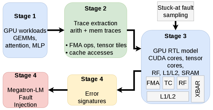</details> Fig. 1: RTL characterization flow for error signature extraction. <details> <summary>2604.10390v1/x2.png Details</summary>  ### Visual Description ## Diagram: Fault Injection Framework for Machine Learning Models ### Overview The diagram illustrates a technical framework for injecting faults into machine learning models during training. It is divided into three sections: 1. **Temporal Injection Parameters** (A) 2. **Spatial and Architectural Parameters** (B) 3. **Fault Density & Bit-Flip Profile** (C) ### Components/Axes #### Section A: Temporal Injection Parameters - **Labels**: - "Fault Injected Rank" (leftmost column, labeled 0, 1, 2, ..., 16) - "Backward Weight Gradients" (orange block) - "Backward Input Gradients" (pink block) - "Forward Output" (blue block) - "Fault Injected Training Phase" (horizontal axis) - "Multi-headed Self-Attention MLPs" (stacked yellow blocks) - "Decoder.layers.7.mlp.fc1" (text annotation) - **Flow**: - Gradients (backward weight/input) and forward outputs are processed through multi-headed self-attention layers. - Fault injection occurs at specific ranks during training phases. #### Section B: Spatial and Architectural Parameters - **Labels**: - "Fault Checkpoint" (vertical colored bars: red, green, blue, etc.) - "Fault Error Rate" (formula: `Error Rate = 5 / (7287 - 2148 + 1)`) - "Fault Injection Tile" (green rectangle with dimensions `N`, `K`, `M`) - **Flow**: - Faults are injected between checkpoints during training iterations. - Error rate determines the number of faulty iterations (5 in this case). #### Section C: Fault Density & Bit-Flip Profile - **Labels**: - "Original Value" (-2.12) - "Faulty Value" (-431.3) - "Error Signature" (sequence of 1s and 0s with red dots) - "Pos: {12, 11, 10, 9, 7}" (bit positions flipped) - **Flow**: - Bit-flips at specific positions alter the original value to a faulty value. ### Detailed Analysis #### Section A - **Fault Injected Rank**: Ranks 0–16 are shown with dashed lines, indicating multiple injection points. - **Gradients**: Backward weight and input gradients are distinct blocks, suggesting separate processing paths. - **Multi-headed Self-Attention**: Stacked layers imply hierarchical processing of gradients and outputs. #### Section B - **Error Rate Calculation**: - `7287 - 2148 + 1 = 5140` - `Error Rate = 5 / 5140 ≈ 0.0009727` (≈0.0973%). - **Checkpoints**: Colored bars (red, green, blue) represent intervals between which faults are injected. #### Section C - **Bit-Flip Impact**: - Original value: -2.12 (binary: `110000000000111101`). - Faulty value: -431.3 (binary: `1101110101011101101`). - Flipped bits at positions 12, 11, 10, 9, 7 (highlighted in green). ### Key Observations 1. **Temporal Injection**: Faults are injected at specific ranks during training phases, affecting gradients and outputs. 2. **Spatial Parameters**: Checkpoints and error rates govern the frequency and scope of fault injection. 3. **Bit-Flip Profile**: A single bit-flip at position 12 causes a drastic change in the value (-2.12 → -431.3), indicating high sensitivity. ### Interpretation - **Model Robustness**: The framework highlights how temporal and spatial parameters influence fault injection, critical for testing model resilience. - **Error Propagation**: The drastic change in value from a single bit-flip suggests vulnerabilities in numerical stability. - **Checkpoint Strategy**: Injecting faults between checkpoints allows controlled testing of recovery mechanisms. - **Architectural Impact**: Multi-headed self-attention layers may distribute fault effects differently than simpler architectures. This diagram provides a structured approach to analyzing fault injection in ML models, emphasizing the interplay between training dynamics, architectural design, and numerical stability. 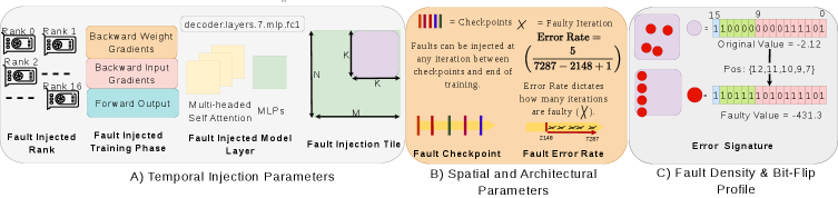</details> Fig. 2: Software level fault site tuple characterized with seven parameters divided in three broad categories: 1) Temporal 2) Spatial and Architectural 3) Fault Intensity & Bit-Level. Figure 1 summarizes our RTL characterization flow. Rather than simulate the full LLM training workload at RTL — which is computationally intractable — we target the GPU functional units most exposed during transformer training: FMA paths in the CUDA cores, tensor cores, register files, and L1/L2 caches and SRAM arrays. Simulations are driven by computation traces extracted directly from the training workload and replayed through a commercial EDA tool to obtain cycle-accurate functional-unit activity under realistic input and toggle conditions. We inject stuck-at faults sampled in proportion to the silicon area of each unit, ensuring the fault population reflects each block’s contribution to the overall GPU design. For each fault, we record its output error signature: the set of affected bits, the magnitude of the numerical deviation, and the corruption pattern at the functional-unit output. These signatures characterize the what of each fault — which bits are affected, at what magnitude, and in what pattern — while the where and when are determined by architectural reasoning about GPU data flow and training dynamics, as described in next subsection. <details> <summary>2604.10390v1/figs/rtl-signatures.png Details</summary>  ### Visual Description ## Heatmap with Histogram Panels: Bit Position Frequency Analysis ### Overview The image consists of three panels (a, b, c), each containing a 16x16 grid with colored squares and a corresponding histogram below. The grids visualize spatial distributions of colored squares, while the histograms quantify frequency distributions across bit positions (0-15). Colors (red, maroon, yellow) represent distinct data categories. ### Components/Axes - **Grids**: - 16x16 matrix with black grid lines - Colored squares (red, maroon, yellow) in specific positions - **Histograms**: - X-axis: "Bit position" (0-15) - Y-axis: "Freq." (frequency) - Bar colors match grid colors (red, maroon, yellow) - **Legends**: Implied by color coding (no explicit legend visible) ### Detailed Analysis #### Panel (a) - **Grid**: - Red squares occupy: - Top-left 4x4 quadrant (rows 0-3, columns 0-3) - Bottom-right 2x2 quadrant (rows 14-15, columns 14-15) - **Histogram**: - Single red bar at bit position 5 - Frequency ≈ 12 (estimated from bar height) - **Spatial Correlation**: Red squares in grid align with bit position 5 in histogram #### Panel (b) - **Grid**: - Maroon squares distributed across: - Diagonal from top-right to bottom-left - Scattered in middle rows (rows 4-10) - **Histogram**: - Multiple maroon bars at: - Bit 3: ≈ 8 - Bit 5: ≈ 6 - Bit 7: ≈ 5 - Bit 9: ≈ 4 - Bit 11: ≈ 3 - Bit 13: ≈ 2 - Bit 15: ≈ 1 - **Spatial Correlation**: Maroon squares map to odd-numbered bit positions #### Panel (c) - **Grid**: - Yellow squares form: - Top row (row 0, columns 0-15) - Bottom row (row 15, columns 0-15) - **Histogram**: - Bell-shaped distribution centered at bit 10 - Frequencies: - Bit 10: ≈ 15 - Bit 9/11: ≈ 12 - Bit 8/12: ≈ 8 - Bit 7/13: ≈ 5 - Bit 6/14: ≈ 3 - Bit 5/15: ≈ 1 - **Spatial Correlation**: Yellow squares in top/bottom rows correspond to bit positions near 10 ### Key Observations 1. **Panel (a)**: Single dominant bit (5) with clustered spatial representation 2. **Panel (b)**: Multiple bits with decreasing frequency (3 > 5 > 7 > ... > 15) 3. **Panel (c)**: Symmetric normal distribution centered at bit 10 4. **Color Consistency**: All histograms use matching colors to their respective grids 5. **Bit Position Mapping**: Grid coordinates correlate with bit positions via: - Row = Bit position (0-15) - Column = Bit value (0-15) ### Interpretation The data demonstrates three distinct bit distribution patterns: 1. **Localized Activation** (Panel a): Single bit (5) dominates with spatial clustering 2. **Sparse Distribution** (Panel b): Odd-numbered bits show decreasing frequency, suggesting structured encoding 3. **Normal Distribution** (Panel c): Symmetric spread around bit 10 indicates random or Gaussian-like bit allocation The histograms validate the spatial patterns in grids, confirming that: - Panel (a) represents a 1-bit system with positional encoding - Panel (b) shows a multi-bit system with priority ordering (lower bit positions more frequent) - Panel (c) demonstrates a balanced bit distribution with central tendency Notable anomalies include the perfect symmetry in Panel (c) and the strict odd-bit pattern in Panel (b), suggesting intentional design rather than random distribution. 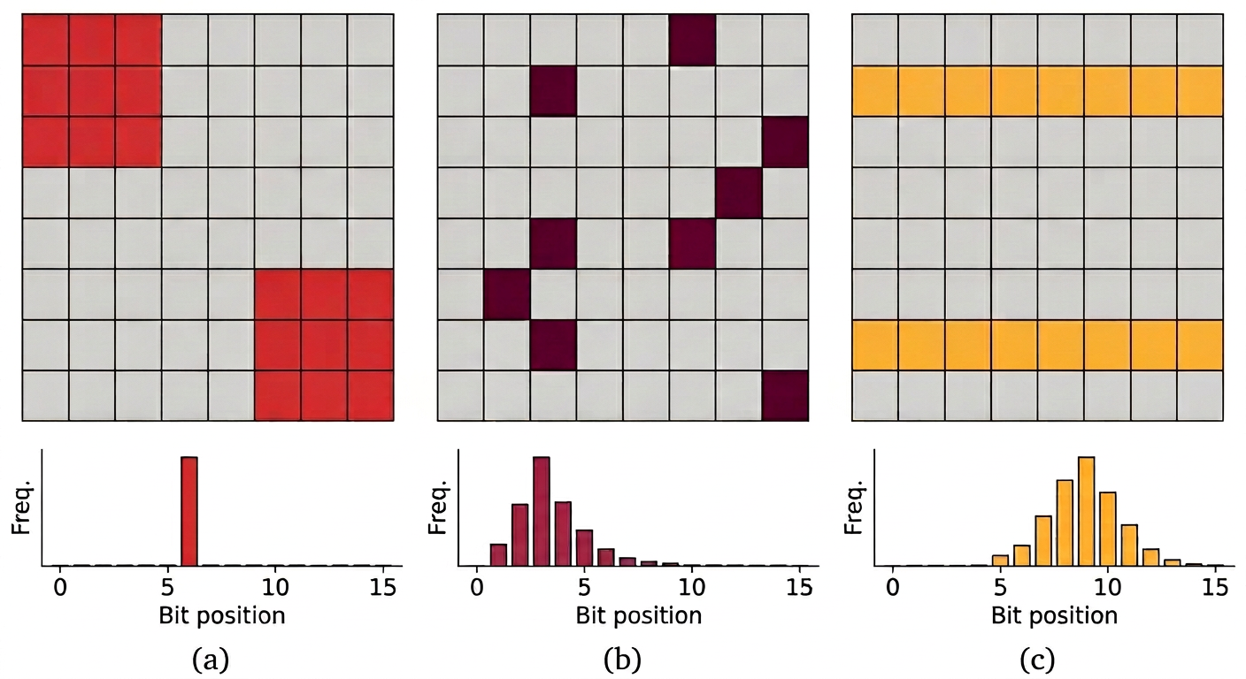</details> Fig. 3: Examples error signatures derived from RTL characterization. The error signatures in Figure 3 are illustrative examples derived from single stuck-at fault RTL simulations. For Figure 3 (a), the fault is injected into a tensor core datapath bit that feeds a subset of output tiles, producing localized $3× 3$ patches in the matrix where all corruptions share the same flipped bit position, resulting in a sharply peaked bit-position distribution. For Figure 3 (b), the fault is injected on an output bit of an FMA ALU, perturbing low- and mid-order bits in a pattern-dependent manner so that most outputs remain correct but a small number of operations exhibit sporadic, high-magnitude numeric outliers with a broader bit distribution. In case (c), the stuck-at fault is in L1 cache line such that an entire matrix row’s stored values are corrupted when accessed, yielding structured row-wise corruption and a wide bit-position distribution centered on high-order bits. We collected over 6,000 such error signatures from faults injected throughout the GPU memory hierarchy and compute datapaths providing a diverse empirical basis for the software-level fault injection. ### III-C Software Fault Site Parameterization RTL fault injection operates on the registers and combinational data paths of a functional unit; the analogous injection targets in a software training loop are the tensors flowing through the computation graph — activations, gradients, and weights. Translating hardware-derived error signatures into this setting requires a structured parameterization that captures the spatial, temporal, and numerical dimensions of a physical defect as quantities controllable within Megatron-LM. The core challenge is that a single stuck-at defect has a fixed physical location, but its effect on training depends on which tensor is being computed, on which device, at which step, and at what numerical precision. A parameterization that spans all of these dimensions lets us reproduce the full diversity of hardware failure modes during distributed training with Megatron-LM. To this end, we define a software-level fault site as a tuple of seven parameters organized into three categories (Figure 2). The fault intensity and bit-level parameters are drawn from the RTL-derived error signature distributions established above; the spatial and architectural parameters follow from first-principles reasoning about how a fixed hardware defect interacts with distributed training computation; and the temporal parameters capture the stochastic activation behavior of intermittent defects, as detailed in Section III-E. The seven parameters are described below: #### III-C 1 Spatial and Architectural Coordinates These three parameters specify which hardware and which part of the model is affected (Figure 2 b). a) Rank identifies the faulty GPU in the distributed cluster, simulating the common datacenter scenario where a single unhealthy device operates alongside otherwise healthy peers. b) Layer pins the fault to a specific transformer layer and sub-module — Multi-Head Attention, MLP, or LayerNorm — enabling study of whether certain components are more susceptible to corruption than others. c) Training Phase determines which tensor is corrupted: forward-pass activations (fwd_outputs), backward-pass input gradients (bwd_grad_inputs), or weight gradients (bwd_grad_weights). The distinction is consequential: an activation error is consumed and discarded, whereas a weight gradient error propagates directly into the model parameters, causing persistent drift in the optimization trajectory. #### III-C 2 Temporal Injection Parameters These two parameters specify when and how often corruption occurs during training. a) Fault Checkpoint sets the iteration at which injection begins, enabling controlled comparisons of model vulnerability at different stages of convergence — early training, when gradients are large and noisy, versus later stages, when the model is near a local minimum and more sensitive to perturbation. b) Error Rate controls the fraction of eligible iterations that experience a fault, spanning the full persistence spectrum: a rate of 1.0 models a permanent stuck-at defect corrupting every iteration, while a low rate models an intermittent defect that activates under specific input or operating conditions. Section III-E describes how this parameter is derived and swept. #### III-C 3 Fault Intensity & Bit-Level Mechanics These two parameters specify the severity and structure of the numerical corruption applied to the target tensor. a) Fault Density controls the proportion of corrupted elements within the target tensor tile. A low density models a localized defect; a higher density models a fault in shared logic — such as a cache line or register file entry — that corrupts multiple values simultaneously. b) Bit-Flip Profile specifies which bits of the floating-point representation are flipped and how many. Flipping an exponent bit can shift a value by orders of magnitude (e.g., $3.141→ 3248$ ), whereas mantissa flips produce minor precision loss. By replaying the bit-flip patterns observed in the RTL error signatures, this parameter anchors the software fault model in hardware-measured corruption rather than uniform random bit-flip assumptions. ### III-D Instantiating a Fault Site: Fixed and Variable Parameters Instantiating the fault-site tuple for a concrete injection campaign requires deciding which of its seven parameters reflect fixed properties of the physical defect and which must be resampled as the data stream changes across iterations. A physical defect is anchored to one location on one device, but the tensor it corrupts, the layer it affects, and the bit pattern it produces all depend on what computation happens to be scheduled on the defective unit. This distinction between defect-level properties and data-stream interactions determines which parameters are initialized once at campaign start and which vary throughout training. #### III-D 1 Fixed Parameters a) Rank is fixed because a hardware defect resides on a specific physical device. A degraded functional unit on GPU $k$ remains faulty for the entire training run, and we assume at most one faulty GPU at any time. b) Fault Checkpoint and c) Error Rate are fixed because they describe the temporal characteristics of the defect rather than any individual corruption event. The checkpoint defines the training window during which the fault is active — modeling, for example, a defect that emerges after thermal stress accumulates over extended operation. The error rate captures how frequently the defect propagates to a visible output error within that window. #### III-D 2 Variable Parameters a) Training Phase is sampled uniformly from fwd_outputs, bwd_grad_inputs, and bwd_grad_weights. This is an architectural choice: the forward pass performs one matrix computation per layer, whereas the backward pass performs two (input and weight gradients), so a uniform draw over three phases yields a natural 2:1 exposure ratio for backward versus forward computation without explicit timing measurements. b) Layer is sampled uniformly across transformer layers. Because layers are structurally identical and occupy the same GPU for comparable durations, uniform sampling reflects equal exposure of a fixed defect to each layer’s computation. c) Fault Injection Tile is sampled to match GPU execution granularity. Matrix operations are executed in fixed-size tiles; a defect corrupts whatever tile is scheduled on the faulty unit at activation. We therefore select a target tile at random and derive the intra-tile corruption pattern from the RTL error signature distributions. d) Bit-Flip Profile is drawn from the RTL error signatures with single-bit flips weighted more heavily than multi-bit patterns. ### III-E Modeling Intermittent Faults With Error Rate <details> <summary>2604.10390v1/x3.png Details</summary>  ### Visual Description ## Bar Chart: Intermittent Fault Activation Across Training Steps ### Overview The top chart visualizes fault activation patterns during training steps for three fault types (r=1.0, r=0.7, r=0.15). Each fault type is represented by horizontal bars segmented into red (corruption) and gray (no corruption), with a legend clarifying fault permanence. ### Components/Axes - **Y-Axis (Fault Type)**: - Labels: `r = 1.0`, `r = 0.7`, `r = 0.15` - Legend: - Red: Corruption (Permanent faults for r=1.0; Intermittent for r=0.7/0.15) - Gray: No corruption - **X-Axis (Training Step)**: - Markers: `0`, `N/4`, `N/2`, `3N/4`, `N` - Scale: Discrete intervals representing training progress. ### Detailed Analysis - **r = 1.0 (Permanent Faults)**: - Entire bar is red, indicating continuous corruption across all training steps. - **r = 0.7 (Intermittent Faults)**: - Segments: Red (corruption) and gray (no corruption) alternate. - Example: At `N/2`, ~25% of the bar is gray (no corruption). - **r = 0.15 (Intermittent Faults)**: - Segments: Red dominates early steps (`0`, `N/4`), with increasing gray segments later (`N/2`, `3N/4`, `N`). ### Key Observations - Higher `r` values correlate with greater persistent corruption. - Lower `r` values show intermittent fault activation, with corruption decreasing as training progresses. ### Interpretation The chart demonstrates that fault permanence (`r=1.0`) leads to unmitigated corruption, while lower `r` values allow partial recovery during training. This suggests adaptive training mechanisms may reduce intermittent faults over time. --- ## Line Graph: Fault PDF vs. Injection Rate ### Overview The bottom graph plots fault probability density function (PDF) against injection rate (`r`), with shaded regions indicating defect categories. ### Components/Axes - **Y-Axis (Fault PDF f(r))**: - Range: 0.0 to 3.5 - **X-Axis (Injection Rate r)**: - Range: 0.0 to 1.0 - **Legend**: - Blue line: Fault PDF curve - Shaded regions: - Green: Latent/Early-Life Defects - Yellow: Marginal Defects - Pink: Silicon Aging Related Defects - Dark pink: Severe Aging ### Detailed Analysis - **Fault PDF Curve**: - Peaks at ~0.2 injection rate (~3.0 PDF value). - Declines sharply as `r` increases beyond 0.4. - **Shaded Regions**: - **Green (Latent/Early-Life Defects)**: Dominates low `r` (0.0–0.4). - **Yellow (Marginal Defects)**: Overlaps with green at mid `r` (0.4–0.6). - **Pink (Silicon Aging)**: Emerges at `r > 0.6`. - **Dark Pink (Severe Aging)**: Minimal contribution (<0.8 `r`). ### Key Observations - Highest fault probability occurs at low injection rates (`r ≈ 0.2`). - Severe aging defects are negligible except at very high `r` (>0.8). ### Interpretation The data implies that low injection rates exacerbate early-life defects, while higher rates shift failure modes toward silicon aging. This aligns with semiconductor reliability models where early stress dominates at low operational thresholds. --- ## Cross-Referenced Insights 1. **Top Chart + Bottom Graph**: - Permanent faults (`r=1.0`) in the top chart may correspond to "Severe Aging" in the bottom graph, as both represent unmitigated failure modes. - Intermittent faults (`r=0.7/0.15`) align with "Marginal Defects" and "Silicon Aging," suggesting partial recovery mechanisms. 2. **Training vs. Operational Context**: - The top chart focuses on training-phase fault dynamics, while the bottom graph models operational defect distributions. ## Final Notes - All legend colors match chart elements (e.g., red = corruption in both charts). - No textual data in non-English languages detected. - Spatial grounding: Legends are positioned at the bottom-left (top chart) and right (bottom graph), ensuring clarity without obscuring data. 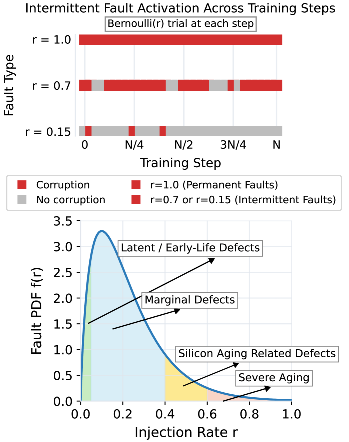</details> Fig. 4: Stochastic Intermittent Fault Activation Model To model intermittent faults — permanent hardware defects that only manifest on a subset of operations — we interpret the error-rate field in the fault tuple as the probability that a given spatial fault site produces a visible corruption during training. Whether a given operation produces a visible error depends on whether the input data exercises the defective logic path, or whether the operating conditions — voltage, frequency, or thermal stress — cross the threshold at which the defect becomes active. This combination of data-dependent and condition-dependent activation is what makes permanent faults behave intermittently at the software level. The error injection rate $r∈(0,1]$ is defined for a given defect as the per-iteration probability that the defect produces a visible corruption at the software level, conditioned on the operation using the faulty resource. In other words, $r$ summarizes the defect’s detectability: the fraction of input patterns that exercise the faulty logic path and propagate an error to architecturally visible state. Each fault tuple is associated with a fixed rate $r$ for the duration of an injection campaign. At each eligible iteration, a Bernoulli trial with parameter $r$ decides whether the defect activates; on activation, the fault tuple is used to inject the error to the target tensor. A rate $r=1.0$ models a hard stuck-at defect that corrupts every eligible operation, whereas $r\ll 1$ models a timing‑marginal or latent defect that rarely manifests. To study how activation frequency shapes training behavior, we treat $r$ as a hyperparameter and sweep it across a broad range. Figure 4 visualizes the fault activation over training steps as a Bernoulli process with rate $r$ , and the the corresponding probability density function $f(r)$ . We construct PDF $f(r)$ based on prior reliability reports: these studies consistently observe that most permanent or intermittent defects activate rarely, while a smaller fraction exhibit much higher activation rates. We therefore choose a unimodal distribution with most probability mass concentrated at low $r$ (latent and marginal defects), but with a long tail covering higher $r$ values corresponding to aging and severely degraded structures. For our experiments, we select a set of representative rates spanning these regions and run separate campaigns at each value, so that each campaign probes a distinct point in this activation-rate design space. This ties the error-rate parameter back to physical intuition about intermittent defects while providing a systematic knob for characterizing how faults of different activation frequencies affect LLM training stability. ## IV Experiment Setup ### IV-A Models and Dataset Models: We perform all fault-injection experiments on the GPT-2 family of decoder-only Transformers [25], using the 124M (GPT-2 Small) and 355M (GPT-2 Medium) variants. These models represent the foundational archetype for modern decoder-only LLMs (e.g., Llama, GPT-4), while remaining small enough to support thousands of full training runs. To study the effect of model scaling under realistic training dynamics, we train both variants from scratch on the WikiText language modeling dataset [21]. This experimental design deliberately trades absolute model size for statistical rigor: by restricting to two GPT-2 architectures, we are able to run 7,664 complete fault-injected pre-training experiments, enabling fine-grained evaluation of a large space of fault sites and activation rates. Dataset: All the experiments are carried out with WikiText [21] dataset and we measure the PPL of all the runs to see the impact of fault injections at the macro level. A rigorous fault injection campaign requires thousands of targeted training iterations to achieve statistical significance across a massive configuration space (layer depth, error rate, data format etc). By utilizing a single, sufficiently complex dataset that thoroughly exercises the model’s computational graph, we eliminate dataset-induced variance as a confounding factor while keeping the computational overhead of exhaustive fault profiling tractable. ### IV-B Data Formats To evaluate the impact of hardware faults across modern mixed-precision regimes, we run all fault-injection campaigns under three training formats: IEEE FP16, BF16 [16], and FP8 [23], which are the de facto low-precision standards. Rather than varying datasets or model sizes, we fix the architecture and data and sweep the numerical format, since the low-level propagation of a bit-flip through PyTorch primitives is governed primarily by the underlying representation. For example, flipping an exponent bit in an FP16 tensor can change a value by orders of magnitude, whereas the same spatial fault in a BF16 tensor, with a wider exponent and narrower mantissa, produces a different corruption profile; FP8 further alters this trade-off by aggressively compressing both range and precision. While increasing model scale is known to affect activation outlier distributions and thus quantization behavior [5], isolating the numerical format at a controlled scale allows us to rigorously probe a large space of hardware-level bit-flips and activation rates, yielding more direct, actionable insight into how representation choice shapes training-time fault sensitivity. ### IV-C Hardware, Software and Training Recipe Hardware: The fault injection training experiments were run on 16× NVIDIA H100 GPUs spread across two 8-GPU nodes, using data-parallel Megatron-LM training. Each experiment occupies all 16 GPUs across both nodes. Software: We utilize the open-source Megatron-LM [26] framework, which we specifically modified to integrate our targeted fault injection methodology during model training. Training Recipe: We employ a standard configuration using the Adam optimizer, linear warmup with cosine annealing, and sequence parallelism for distributed workloads. Across all configurations, this setup yields 7,664 complete fault-injected pre-training runs from scratch (4,681 for GPT-2 Small and 2,983 for GPT-2 Medium), in which RTL-derived error signatures are used to construct the fault-site tuples and the error-rate parameter is swept across its range. ## V Results <details> <summary>2604.10390v1/x4.png Details</summary>  ### Visual Description ## Multi-Panel Figure: Training Dynamics and Fault Injection Analysis ### Overview The image presents a multi-panel technical analysis of model training dynamics under various fault injection scenarios. It includes four line graphs (1a-d), a weight divergence comparison (2), and two bar charts (3a-b) comparing fault simulation frequencies across model sizes. ### Components/Axes **1) Training Loss Dynamics (Subplots 1a-1d):** - **X-axis**: Training iteration (0-8000) - **Y-axis**: Loss value (2-6) - **Legends**: Located top-left of each subplot - Fault-free reference (dotted line, loss=3.352, PPL=28.54) - NaN loss iterations (red triangles) - **Subplot Labels**: - (a) Spike-and-Recover (rate=0.01, PPL=28.54) - (b) Spike-and-Degrade (rate=0.5, PPL=161.66) - (c) Silent Degradation (rate=1, PPL=31.71) - (d) Gradual Drift (rate=1, PPL=29.42) **2) Weight Divergence Comparison (Subplot 2):** - **X-axis**: Training iteration (0-6000) - **Y-axis**: L2 norm of weight difference (0-10) - **Legend**: Top-left, color-coded fault rates (0.001-1.0) - **Lines**: - Dashed: Fault-free baseline - Solid: Fault-injected scenarios (rates 0.001-1.0) **3) Fault Simulation Frequencies (Subplots 3a-3b):** - **X-axis**: Fault types (Spike Recover, Spike Degrade, Silent Degradation, Gradual Drift) - **Y-axis**: Percentage of simulations (%) - **Models**: - (a) GPT-2 Small - (b) GPT-2 Medium - **Colors**: Green (Spike Recover), Orange (Spike Degrade), Red (Silent Degradation), Blue (Gradual Drift) ### Detailed Analysis **1a-1d Training Loss Trends:** - **1a (Spike-and-Recover)**: Green line remains flat at ~3.35 loss (PPL=28.54), matching fault-free reference - **1b (Spike-and-Degrade)**: Orange line spikes to ~5.5 loss at iteration 1000, then stabilizes (PPL=161.66) - **1c (Silent Degradation)**: Red line shows initial fluctuation (~4.5 loss) before stabilizing (PPL=31.71) - **1d (Gradual Drift)**: Blue line maintains constant ~3.5 loss (PPL=29.42) **2) Weight Divergence:** - Fault-free baseline (dashed) remains near 0 - Fault-injected lines show: - Rate 0.001: Minimal divergence (~1.5) - Rate 1.0: Sharp increase to ~8.5 divergence - Color progression: Blue (lowest rate) to Red (highest rate) **3a-3b Fault Simulation Frequencies:** - **GPT-2 Small**: - Spike Recover: 6.1% - Spike Degrade: 9.5% - Silent Degradation: 1.5% - Gradual Drift: 0.9% - **GPT-2 Medium**: - Spike Recover: 4.7% - Spike Degrade: 6.4% - Silent Degradation: 2.9% - Gradual Drift: 4.1% ### Key Observations 1. **Fault Rate Impact**: Higher fault rates correlate with increased loss (1b: 0.5→161.66 PPL) and weight divergence (2: 0.001→1.0 rate) 2. **Model Robustness**: GPT-2 Small shows higher fault simulation frequencies than Medium across all fault types 3. **Training Stability**: Gradual Drift (1d) maintains most stable loss despite high fault rate (1.0) 4. **Anomaly**: Silent Degradation (1c) achieves lower PPL (31.71) than Gradual Drift (29.42) despite similar fault rates ### Interpretation The data demonstrates that: - **Training Method Sensitivity**: Spike-and-Degrade (1b) exhibits catastrophic failure (highest PPL) under moderate fault rates, while Gradual Drift (1d) maintains stability - **Fault Injection Correlation**: Weight divergence increases exponentially with fault rate (2), suggesting fault tolerance degrades with higher error rates - **Model Architecture Differences**: GPT-2 Small's higher fault simulation frequencies (3a-b) indicate reduced robustness compared to Medium variant - **Unexpected Finding**: Silent Degradation (1c) achieves better PPL than Gradual Drift despite similar fault rates, suggesting different failure modes This analysis reveals critical insights into model robustness under fault conditions, with implications for fault-tolerant training methodologies and model architecture design. 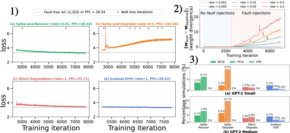</details> Fig. 5: Training loss traces for four representative failure modes under permanent fault injection. Each subplot shows loss over training iterations (GPT2-Small with BF16 format); the dashed line is the fault-free baseline (3.352 nats / PPL = 28.54) and red triangles mark iterations where the loss calculation produced a NaN. Plot 1: (a)Spike-and-Recover: sparse NaN events are absorbed and the run converges to baseline. (b)Spike-and-Degrade: dense NaN events overwhelm recovery and loss diverges. (c)Silent Degradation: no NaN events, yet loss settles above baseline; the most operationally deceptive mode. (d)Gradual Drift: loss is visually indistinguishable from baseline while parameters are silently corrupted. Plot 2: Global weight divergence ( $\|W_fault-W_baseline\|_2$ ) over training, for GPT-2Small with BF16. All fault rates produce monotonically increasing divergence after injection begins. Plot3: Distribution of the four failure modes across data formats and model scales. FP8 produces no Silent Degradation or Gradual Drift. Its outcomes are strictly binary (recover or crash). FP16 shows the highest Spike-and-Degrade fraction, consistent with its wider dynamic range enabling large-but-finite corruptions. ### RQ1: How do permanent faults propagate through training, and what makes them different from transient faults? Prior studies on transient faults during training typically inject a single bit flip and observes whether the training recovers or crashes [30, 2]. This probes resilience to a one-time perturbation, but not the behavior of a GPU that persistently corrupts computations over hundreds of thousands of iterations. Our pre-training runs are subjected to permanent fault injection, revealing four qualitatively distinct failure modes (Plot 1 in Figure 5), only the first of which would be observable under a transient fault model. 1) Spike-and-recover. At low fault rates, corruptions are too infrequent to overwhelm the training dynamics. Each NaN event triggers mixed-precision recovery (loss-scale reduction and update skipping [22]), after which gradient descent proceeds with predominantly clean updates. The loss therefore exhibits isolated spikes followed by return to the fault-free trajectory. This is the regime that single-injection studies capture and typically interpret as training is resilient to the injected fault. 2) Spike-and-degrade. At higher fault rates, NaN events become sufficiently frequent that the loss scale collapses and the skip-and-halve mechanism no longer restores stability. The optimizer is effectively stalled: many steps are skipped, the effective learning signal vanishes, and the loss rises monotonically as corrupted activations repeatedly propagate through the network. In contrast to spike-and-recover, fault rate here exceeds the threshold at which training dynamics can self-heal. 3) Silent degradation. Faults are frequent and severe enough to corrupt the training state, but not enough to crash the job or consistently produce NaNs. Each faulty iteration perturbs activations or gradients while remaining finite, so weights are updated using biased signals and the loss drifts upward over time. The run completes without obvious instability indicators, making this behavior operationally difficult to detect. 4) Gradual drift. Faults predominantly affect backward-pass quantities (e.g., gradient inputs), introducing small but systematic errors into each update step. These biases accumulate over long horizons, leading to a slow divergence from the fault-free trajectory without sharp loss spikes or NaNs. This mode is invisible to NaN-based monitoring and unlikely to be exposed by short fine-tuning runs, but becomes apparent over full pre-training durations. Weight divergence reveals what loss curves hide: Plot 1 in Figure 5 shows the loss trajectories that a practitioner would observe, whereas Plot 2 reports the L2 distance between the faulty and fault-free parameter vectors throughout training. All permanent fault runs exhibit monotonically increasing parameter divergence once injection begins; the model does not rejoin the baseline trajectory. Runs with error rates $r≤ 0.005$ remain near-zero divergence, consistent with benign perplexity outcomes, while runs with $r≥ 0.01$ show steadily growing distance. Notably, even trajectories whose loss remains near baseline (Gradual Drift) accumulate substantial weight drift, indicating that loss alone can mask significant deviations in the training parameters. Failure mode prevalence across formats: Plot 3 summarizes how the four failure modes distribute across numerical formats and model scales. Two effects are most prominent: FP8 produces no instances of Silent Degradation or Gradual Drift: outcomes are effectively binary (recover or crash), which is consistent with its narrow dynamic range forcing faults either to saturate harmlessly or to trigger NaNs; in contrast, FP16 exhibits the largest fraction of Spike-and-degrade runs - its wider dynamic range permits large but finite corruptions that degrade the model without necessarily causing a crash. These format-dependent patterns indicate that numerical representation is a first-order determinant of how permanent faults manifest at the training-loss level. <details> <summary>2604.10390v1/x5.png Details</summary>  ### Visual Description ## Bar Chart: Model Performance Comparison Across Precision Formats ### Overview The chart compares the performance of GPT-2 Small and Medium models across three precision formats (FP16, BF16, FP8) using three metrics: Model PPL, NaN/Inf in Loss Calculation, and NaN/Inf in Weights or Activations. Data is presented as percentages of experiments across three categories: Unchanged (≤1%), Changed (>1%), and Crashed. ### Components/Axes - **X-Axis**: Categories (Unchanged (≤1%), Changed (>1%), Crashed) - **Y-Axis**: Percentage of experiments (%) - **Legend**: - FP16 (blue) - BF16 (orange) - FP8 (green) - **Subsections**: - (a) GPT-2 Small - (b) GPT-2 Medium ### Detailed Analysis #### (a) GPT-2 Small 1. **Model PPL**: - **Unchanged (≤1%)**: FP16 (72.3%), BF16 (66.8%), FP8 (57.5%) - **Changed (>1%)**: FP16 (11.0%), BF16 (6.3%), FP8 (0.5%) - **Crashed**: FP16 (16.7%), BF16 (26.9%), FP8 (41.9%) 2. **NaN/Inf in Loss Calculation**: - FP16 (14.6%), BF16 (15.9%), FP8 (25.6%) 3. **NaN/Inf in Weights or Activations**: - FP16 (15.7%), BF16 (16.8%), FP8 (24.5%) #### (b) GPT-2 Medium 1. **Model PPL**: - **Unchanged (≤1%)**: FP16 (76.5%), BF16 (69.6%), FP8 (64.1%) - **Changed (>1%)**: FP16 (13.8%), BF16 (10.0%), FP8 (0.8%) - **Crashed**: FP16 (9.6%), BF16 (20.4%), FP8 (35.1%) 2. **NaN/Inf in Loss Calculation**: - FP16 (14.0%), BF16 (11.4%), FP8 (17.9%) 3. **NaN/Inf in Weights or Activations**: - FP16 (19.5%), BF16 (23.3%), FP8 (22.4%) ### Key Observations 1. **FP8 Consistently Higher Crash Rates**: - In both models, FP8 has the highest percentages in the "Crashed" category (41.9% for Small, 35.1% for Medium), suggesting lower numerical stability. 2. **FP16 Dominates Unchanged States**: - FP16 shows the highest percentages in "Unchanged (≤1%)" for both models (72.3% and 76.5%), indicating better stability in maintaining small changes. 3. **BF16 as a Middle Ground**: - BF16 generally falls between FP16 and FP8 in all metrics, with moderate performance across categories. 4. **FP8 Higher NaN/Inf in Loss Calculation**: - FP8 has the highest NaN/Inf rates in loss calculation (25.6% for Small, 17.9% for Medium), highlighting potential precision-related issues. ### Interpretation The data suggests that **FP8 precision introduces greater numerical instability** compared to FP16 and BF16, as evidenced by higher crash rates and NaN/Inf occurrences. FP16 demonstrates superior stability in maintaining unchanged states but underperforms in crash resilience. BF16 balances performance but does not outperform FP16 in critical metrics. These trends imply that lower-precision formats (FP8) may require additional safeguards for reliable model execution, while FP16 remains the most stable choice for minimizing numerical errors. 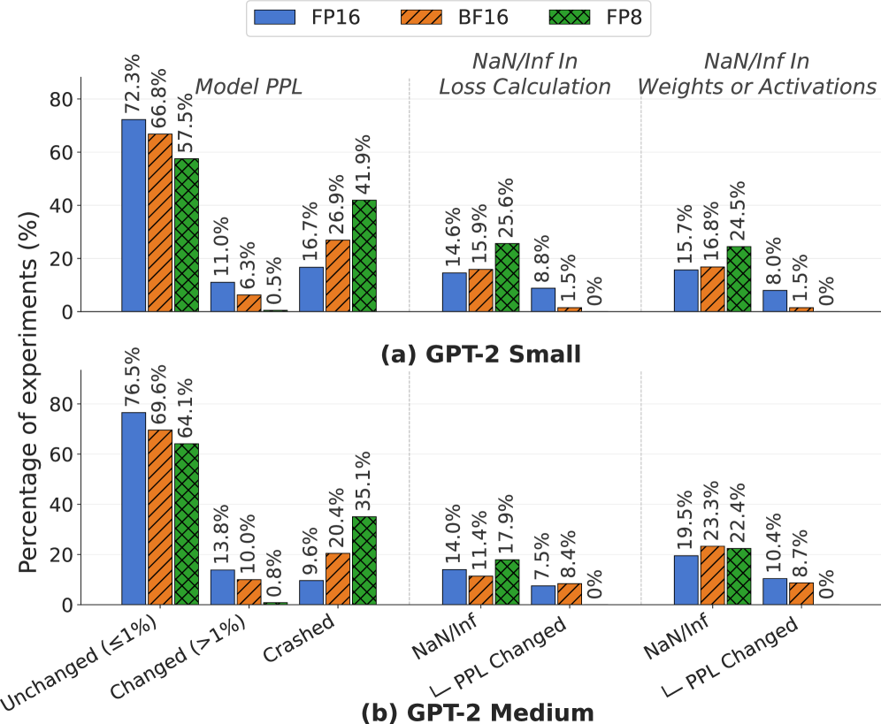</details> Fig. 6: Distribution of training outcomes under permanent fault injection across data formats for GPT2-Small(a) and GPT2-Medium(b). Left: final model PPL classified as Unchanged, Changed, or Crashed. Middle and right: fraction of runs encountering NaN/Inf in loss or weights/activations, with sub-bars showing the subset that also resulted in a PPL change. Lower-precision formats crash more but degrade silently less; larger models show a higher fraction of silent degradation. ### RQ2: How resilient is LLM training to permanent faults? 1) Model training dynamics under fault. We first characterize the impact of fault injection along three complementary dimensions summarized in Figure 6. The primary dimension is final model quality: we measure the perplexity (PPL) of the trained model and classify each run as Unchanged (PPL within 1% of the fault-free baseline of 28.54), Changed (PPL deviates by more than 1%), or Crashed (training does not produce a valid PPL). The 1% threshold is empirically motivated: repeated fault-free runs exhibit up to 1% natural variance, so smaller deviations cannot be confidently attributed to faults. The second dimension records whether the training loss becomes NaN or Inf at any iteration, indicating a breakdown of the optimization objective. The third dimension tracks NaN/Inf events in weights or activations, capturing instability propagating through the network independently of the loss. For the latter two dimensions, a sub-bar reports what fraction of affected runs also exhibit a PPL change, linking low-level numerical faults to observable model degradation. Across all formats, the dominant trend is that LLM training is remarkably resilient to permanent hardware faults: 57–76% of runs complete with PPL indistinguishable from the fault-free baseline. Model behavior under failure, however, depends strongly on numerical precision. For GPT-2 Small, FP16’s remaining 28% of runs split between graceful degradation (11.0% PPL Changed) and crashes (16.7%), with NaN/Inf loss events (14.6%) serving as the primary propagation pathway: roughly 60% of FP16 runs that encounter a NaN/Inf loss still finish training but with elevated PPL. BF16 and FP8 follow a different pattern: crash rates rise to 26.9% and 41.9%, while the fraction showing non-crashing PPL degradation falls to 6.3% and 0.5%. This inverse relationship between crash rate and PPL-change rate reflects a shift in failure mode: lower-precision formats have narrower dynamic ranges, so faults that overflow to NaN typically produce catastrophic failure rather than recoverable, but degraded, solutions. Consequently, in BF16 and FP8, NaN/Inf loss events almost always correspond to either a full crash or a near-baseline outcome, with little middle ground. The same trend appears for NaN/Inf in weights and activations, which closely track loss instability across formats, indicating that faults originate in the computational layers and propagate upward into the loss. GPT-2 Medium (Figure 6 b) exhibits a similar qualitative pattern but with a larger Changed fraction (13.8% for FP16 vs. 11.0% for Small), suggesting that larger models provide more opportunities for faults to induce silent degradation rather than crashes. 2) Impact on PPL. 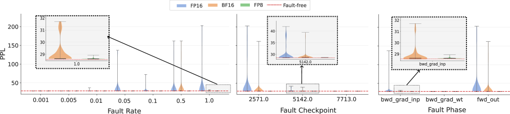We next examine which fault parameters drive variation in model quality. Figure 8 reports the distribution of final PPL for fault-injected runs, stratified by fault rate, injection checkpoint, and fault phase for FP16, BF16, and FP8; the fault-free baseline is PPL = 28.54. The following observations summarize the main trends: 1. Most runs survive, but tail risk is severe. Across all formats, the majority of runs converge near the baseline. For FP16 at fault rate 1.0, the median PPL is 28.58, yet the 95th percentile reaches 192.4, corresponding to converged but poor solutions rather than outright divergence. Permanent faults can therefore silently degrade models without triggering obvious failures. 1. Low fault rates are benign. At rates 0.001 through 0.01, PPL is statistically indistinguishable from the baseline across all three formats. Degradation appears only at rates 0.05 and above, consistent with the optimizer absorbing infrequent corruptions through subsequent updates. Format-dependent differences in distributional spread become pronounced at higher rates. 1. Earlier faults cause more damage. Faults injected at step 2571 yield broader PPL distributions than those at steps 5142 or 7713. Early in training, the model has not yet reached a stable region of the loss landscape and is therefore more sensitive to perturbations. 1. Backward weight gradients are resilient; forward outputs and backward input gradients are not. Faults in bwd_grad_wt have little effect on PPL, due to two mitigating factors: optimizer momentum smooths corrupted gradients over multiple steps, and in distributed training, gradients are averaged across GPUs, diluting the impact of a single faulty rank by a factor of $1/N$ . In contrast, faults in fwd_out and bwd_grad_inp act on local computation before any cross-rank communication and thus propagate without attenuation. 3) Downstream performance. 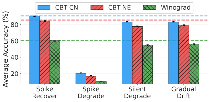Perplexity is an imperfect proxy for task performance: models with similar PPL can differ substantially on downstream evaluations [20]. To test whether training-time corruption from permanent faults translates into real capability loss, we evaluate GPT-2 Medium models using the LM Evaluation Harness [8] on the Children’s Book Test (CBT) [13] and the Winograd Schema Challenge [17]. GPT-2 Small is excluded as it lacks sufficient capacity to produce meaningful scores on these tasks. Figure 7 shows that downstream degradation is not confined to runs with obviously corrupted loss curves. The Spike-and-degrade models perform poorly across all benchmarks. The Spike-and-recover and Gradual Drift models, which maintain near-baseline PPL, still exhibit measurable accuracy drops on both tasks. These results confirm that permanent faults can harm learned representations in ways that are not visible in training perplexity alone, and that loss-curve monitoring is insufficient to detect all forms of training-time corruption induced by faulty hardware. <details> <summary>2604.10390v1/x6.png Details</summary>  ### Visual Description ## Bar Chart: Average Accuracy Comparison Across Degradation Scenarios ### Overview The chart compares the average accuracy (%) of three methods (CBT-CN, CBT-NE, Winograd) across four degradation scenarios: Spike Recover, Spike Degrade, Silent Degrade, and Gradual Drift. Accuracy is measured on a 0-100% scale, with horizontal reference lines at 60% (green) and 85% (blue). ### Components/Axes - **X-axis**: Degradation scenarios (Spike Recover, Spike Degrade, Silent Degrade, Gradual Drift) - **Y-axis**: Average Accuracy (%) with gridlines at 20%, 40%, 60%, 80%, 100% - **Legend**: - Blue: CBT-CN - Red (striped): CBT-NE - Green (crosshatched): Winograd - **Reference Lines**: - Blue dashed line at ~85% (top) - Green dashed line at ~60% (middle) ### Detailed Analysis 1. **Spike Recover**: - CBT-CN: ~85% ±2% (blue bar) - CBT-NE: ~82% ±1% (red bar) - Winograd: ~60% ±3% (green bar) 2. **Spike Degrade**: - CBT-CN: ~20% ±3% (blue bar) - CBT-NE: ~15% ±2% (red bar) - Winograd: ~5% ±1% (green bar) 3. **Silent Degrade**: - CBT-CN: ~82% ±2% (blue bar) - CBT-NE: ~78% ±1% (red bar) - Winograd: ~55% ±2% (green bar) 4. **Gradual Drift**: - CBT-CN: ~83% ±1% (blue bar) - CBT-NE: ~79% ±1% (red bar) - Winograd: ~57% ±2% (green bar) ### Key Observations - **CBT-CN** consistently achieves the highest accuracy across all scenarios, with a notable drop in Spike Degrade (~20%) compared to other scenarios (~80%+). - **CBT-NE** maintains second-place performance in all categories, with the smallest gap vs. CBT-CN in Silent Degrade (~4% difference). - **Winograd** underperforms significantly in Spike Degrade (~5%) but shows moderate improvement in other scenarios (~55-60%). - The blue reference line (~85%) aligns with CBT-CN's performance in Spike Recover and Gradual Drift, suggesting this is a benchmark threshold. - The green reference line (~60%) matches Winograd's performance in Spike Recover, indicating a potential baseline for this method. ### Interpretation The data demonstrates that **CBT-CN and CBT-NE** exhibit superior robustness to degradation compared to Winograd, particularly in degradation scenarios. The dramatic drop in accuracy for all methods during Spike Degrade suggests sudden perturbations (e.g., abrupt input changes) disproportionately impact performance. CBT-CN's consistent top performance implies it may incorporate more effective degradation mitigation strategies, while Winograd's lower scores highlight potential limitations in handling dynamic input variations. The reference lines indicate that achieving >85% accuracy represents exceptional performance, while >60% may represent a minimum acceptable threshold for practical applications. Notably, the similar performance of CBT-CN and CBT-NE across scenarios suggests they share core architectural strengths, with CBT-CN possibly optimizing specific components for marginal gains. Winograd's crosshatched pattern visually distinguishes it as the weakest performer, particularly in degradation contexts. </details> Fig. 7: Performance of faulty GPT2-Medium (BF16) models on downstream tasks. We classify the models in the four categories and run them on Children’s Book Test Dataset [13] (CN = Common Nouns and NE = Named Entities) and Winograd Schema Challenge [17]. We can see that even for cases like spike recover or gradual drifts, the downstream performance is inferior to that of the fault free baselines on downstream tasks due to a change in the training dynamics. ### RQ3: How does the choice of numerical data format influence the resilience of LLM training to permanent hardware faults? <details> <summary>2604.10390v1/x7.png Details</summary>  ### Visual Description ## Line/Scatter Chart: Fault Rate vs. PPL Across Checkpoints and Phases ### Overview The image presents three side-by-side panels analyzing the relationship between fault rates/checkpoints/phases and PPL (likely "Pass/Fail/Likelihood" or a similar metric). Each panel includes a main plot and an inset highlighting specific distributions. The legend at the top identifies four data series: FP16 (blue), BF16 (orange), FP8 (green), and Fault-free (red dashed line). --- ### Components/Axes 1. **Panel 1: Fault Rate** - **X-axis**: Fault Rate (logarithmic scale, 0.001 to 1.0) - **Y-axis**: PPL (0 to 200) - **Legend**: FP16 (blue), BF16 (orange), FP8 (green), Fault-free (red dashed) 2. **Panel 2: Fault Checkpoint** - **X-axis**: Fault Checkpoint (linear scale, 2571.0 to 7713.0) - **Y-axis**: PPL (0 to 40) - **Legend**: FP16 (blue), BF16 (orange), FP8 (green), Fault-free (red dashed) 3. **Panel 3: Fault Phase** - **X-axis**: Fault Phase (categorical: `bwd_grad_inp`, `bwd_grad_wt`, `fwd_out`) - **Y-axis**: PPL (0 to 35) - **Legend**: FP16 (blue), BF16 (orange), FP8 (green), Fault-free (red dashed) --- ### Detailed Analysis #### Panel 1: Fault Rate - **FP16 (blue)**: Distribution peaks at ~0.05 Fault Rate with PPL ~50. Long tails extend to 0.1 (PPL ~150) and 0.01 (PPL ~20). - **BF16 (orange)**: Bimodal distribution: sharp peak at ~0.01 (PPL ~30) and a smaller peak at ~0.1 (PPL ~100). - **FP8 (green)**: Single peak at ~0.1 Fault Rate (PPL ~30). - **Fault-free (red dashed)**: Flat line at PPL ~30 across all Fault Rates. - **Inset**: Zoomed view of FP16 and BF16 distributions. FP16 spans 29–32 PPL at 0.01 Fault Rate; BF16 peaks at 31 PPL at 0.01. #### Panel 2: Fault Checkpoint - **FP16 (blue)**: Single peak at 5142.0 Checkpoint (PPL ~35). - **BF16 (orange)**: Sharp peak at 5142.0 (PPL ~40), with a secondary peak at 7713.0 (PPL ~30). - **FP8 (green)**: Minimal presence; flat line near 30 PPL. - **Fault-free (red dashed)**: Flat line at ~30 PPL. - **Inset**: Highlights FP16 and BF16 peaks at 5142.0 (PPL 30–40) and 7713.0 (PPL ~30). #### Panel 3: Fault Phase - **FP16 (blue)**: Peak at `bwd_grad_wt` (PPL ~35). - **BF16 (orange)**: Peak at `bwd_grad_inp` (PPL ~32). - **FP8 (green)**: Minimal presence; flat line near 30 PPL. - **Fault-free (red dashed)**: Flat line at ~30 PPL. - **Inset**: Zoomed view of `bwd_grad_inp` (29–32 PPL) and `bwd_grad_wt` (30–35 PPL). --- ### Key Observations 1. **Fault Rate Sensitivity**: - BF16 shows the highest sensitivity to low Fault Rates (0.01), with PPL spiking to ~31. - FP16 and FP8 exhibit higher PPL at moderate Fault Rates (0.05–0.1). 2. **Checkpoint Impact**: - Checkpoint 5142.0 is a critical failure point for BF16 (PPL ~40) and FP16 (PPL ~35). - Checkpoint 7713.0 shows reduced PPL for BF16 (~30) but not FP16. 3. **Phase Vulnerabilities**: - `bwd_grad_wt` (FP16) and `bwd_grad_inp` (BF16) are the most failure-prone phases. - `fwd_out` has minimal impact across all configurations. 4. **Fault-free Baseline**: - All configurations maintain a baseline PPL of ~30 when no faults are present. --- ### Interpretation The data suggests that **BF16** is most vulnerable to low Fault Rates (0.01) and specific checkpoints (5142.0), while **FP16** struggles with moderate Fault Rates (0.05–0.1) and phases like `bwd_grad_wt`. The **Fault-free** baseline indicates a consistent performance floor (~30 PPL), implying that faults amplify errors disproportionately. The insets emphasize localized failure modes, such as FP16's bimodal distribution at 0.01 Fault Rate and BF16's sharp peak at Checkpoint 5142.0. These patterns highlight configuration-specific weaknesses, guiding targeted optimizations for fault resilience. </details> Fig. 8: Variation in PPL studied against fault rate, fault checkpoint and fault phase. We can see that as the fault rate increases, we can see a variation in the PPL. Also, earlier the fault is injected, higher chances that it will manifest as a change in PPL. And, when faults are injected in the gradients wrt inputs or the forward pass, we see a higher change in PPL. Data format strongly modulates resilience: FP8 $>$ BF16 $>$ FP16. Figure 8 shows a pronounced difference in PPL distributional spread across numerical formats. FP16 exhibits the widest distributions and most extreme outliers, especially at high fault rates. BF16 yields substantially tighter distributions under the same fault conditions, and FP8 is the most compact of the three. This ordering aligns with the structural properties of the formats: FP16 uses 1 sign, 5 exponent, and 10 mantissa bits, so a single exponent bit-flip can induce a large-magnitude change. BF16 retains 8 exponent bits but only 7 mantissa bits, matching the dynamic range of FP32 and reducing the worst-case impact of individual bit corruptions. FP8 further narrows the effective dynamic range, which bounds the magnitude of individual corruption events and provides a degree of fault containment at the cost of reduced numerical precision. 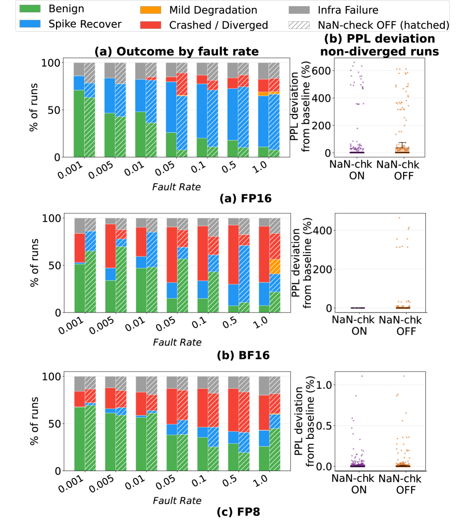### RQ4: How effective is loss-NaN checking in reducing the impact of permanent faults on training dynamics? <details> <summary>2604.10390v1/x8.png Details</summary>  ### Visual Description ## Bar Charts with Scatter Plots: Fault Rate Outcomes and PPL Deviation ### Overview The image presents three comparative analyses (FP16, BF16, FP8) of system outcomes across varying fault rates (0.001 to 1.0). Each section includes: 1. A stacked bar chart showing outcome distributions by fault rate 2. A scatter plot comparing PPL deviation from baseline with NaN-check status ### Components/Axes **Legend (Top-left):** - Green: Benign - Orange: Mild Degradation - Blue: Spike Recover - Red: Crashed/Diverged - Gray: Infra Failure - Hatched: NaN-check OFF **Bar Chart Axes:** - X-axis: Fault Rate (0.001, 0.005, 0.01, 0.05, 0.1, 0.5, 1.0) - Y-axis: % of runs (0-100%) **Scatter Plot Axes:** - X-axis: Fault Rate (0.001-1.0) - Y-axis: PPL deviation from baseline (%) - Categories: NaN-check ON (left), NaN-check OFF (right) ### Detailed Analysis **FP16 Section:** - **Bar Chart Trends:** - At 0.001 fault rate: ~65% Benign (green), ~25% Spike Recover (blue), ~10% Crashed (red) - At 1.0 fault rate: ~15% Benign, ~35% Crashed, ~40% Spike Recover - **Scatter Plot:** - NaN-check ON: Points cluster near 0-100% deviation - NaN-check OFF: Points show higher spread (up to 600% deviation) **BF16 Section:** - **Bar Chart Trends:** - At 0.01 fault rate: ~50% Benign, ~30% Spike Recover, ~20% Crashed - At 0.5 fault rate: ~20% Benign, ~50% Crashed, ~30% Spike Recover - **Scatter Plot:** - NaN-check OFF shows systematic increase in deviation with fault rate **FP8 Section:** - **Bar Chart Trends:** - At 0.1 fault rate: ~40% Benign, ~40% Spike Recover, ~20% Crashed - At 1.0 fault rate: ~10% Benign, ~60% Crashed, ~30% Spike Recover - **Scatter Plot:** - NaN-check OFF points show exponential deviation growth ### Key Observations 1. **Fault Rate Correlation:** - Benign outcomes decrease monotonically with increasing fault rate (FP16: 65%→15%, BF16: 50%→20%, FP8: 40%→10%) - Crashed/Diverged outcomes increase sharply after 0.1 fault rate (FP8: 20%→60%) 2. **NaN-check Impact:** - OFF condition consistently shows higher PPL deviations (FP16: up to 600%, BF16: up to 400%, FP8: up to 100%) - ON condition maintains tighter deviation clusters (<200%) 3. **Color Consistency:** - Red segments (Crashed) dominate at high fault rates (FP8 1.0: 60% red) - Hatched patterns (NaN-check OFF) appear only in scatter plots ### Interpretation The data demonstrates a clear degradation cascade: 1. **System Stability:** Higher fault rates correlate with increased system failures (Crashed/Diverged), suggesting threshold effects at 0.1-0.5 fault rates 2. **Error Propagation:** NaN-check OFF condition amplifies performance deviations, particularly in FP16 (600% max deviation) and BF16 (400% max) 3. **Recovery Mechanisms:** "Spike Recover" category acts as a buffer zone between benign and catastrophic failure, becoming more prominent at moderate fault rates (0.05-0.5) The consistent pattern across all three architectures (FP16, BF16, FP8) indicates fundamental limitations in fault tolerance that NaN-check mechanisms help mitigate. The exponential deviation growth in FP8's scatter plot suggests architectural sensitivity to error propagation mechanisms. </details> Fig. 9: Effect of the loss NaN check across data formats. Left: outcome distribution by fault rate with NaN check enabled (solid) and disabled (hatched). Right: PPL deviation of non-diverged runs under both conditions. For FP16, the check converts many crashes into Spike-and-Recover events but extreme silent degradation persists. For BF16, the check mitigates both crashes and silent degradation. For FP8, outcomes are binary regardless of the check, with PPL deviations under 1%. The loss-NaN check is a standard mixed-precision safeguard: when a NaN or Inf is detected in the loss, the optimizer step is skipped and the dynamic loss scale is halved. We compare the training dynamics of all the three data formats under permanent faults and present our results in Figure 9. For FP16, the failure spectrum is broad: Crashed/Diverged, Spike-and-recover, and Mild Degradation all appear across fault rates. With the NaN check enabled, Spike-and-recover (blue) becomes the dominant non-benign outcome, whereas without it Crashed/Diverged (red) dominates for rates $≥ 0.05$ . This indicates that, for FP16, the check successfully intercepts a substantial fraction of training anomalies that would otherwise be fatal. A particularly consequential effect is that non-diverged FP16 runs exhibit PPL deviations of up to $∼$ 600% above baseline (rightmost panel of Figure 9 a), representing the largest silent degradation among all formats. The NaN check substantially tightens this distribution, but extreme outliers remain, indicating that some fault-induced corruptions accumulate below the NaN threshold and manifest as degraded model quality rather than as a detectable crash. BF16 training (Figure 9 b) exhibits a distinct risk profile that combines unfavorable aspects of both FP8 and FP16. Crash rates at high fault rates approach those of FP8, yet non-diverged runs can still suffer silent PPL degradation of up to $∼$ 400%, a failure mode largely absent in FP8. The NaN check mitigates both classes of failure: it reduces Crashed/Diverged outcomes and suppresses the large PPL deviations among surviving runs. This dual effect makes the check particularly important for BF16: disabling it increases outright failures and exposes training to a class of invisible quality loss that neither crashes nor triggers obvious alarms. As in FP16, the check mainly converts otherwise fatal trajectories to Spike-and-recover behavior rather than eliminating underlying faults. Cross-format summary. FP8 fault outcomes are effectively binary: runs either absorb faults or diverge, so the NaN check primarily prevents crashes. FP16 training is most prone to persistent PPL degradation among surviving runs; the check reduces but does not eliminate this risk. BF16 combines high crash susceptibility with substantial silent degradation, both of which the check mitigates. Across formats and fault rates, fault phase is a stronger predictor of outcome than NaN checking: Forward Output and Backward Gradient Input faults consistently yield the highest crash rates ( $∼$ 60%) at matched fault rates), whereas Backward Gradient Weight faults are largely self-correcting. This phase dependence appears format-agnostic, suggesting it is driven by gradient-flow structure rather than by the numerical representation. ## VI Limitations First, our evaluation is limited to relatively small-scale models, which may differ from the massive foundation models deployed in production clusters. We intentionally accept this trade-off: smaller models allow thousands of full training runs across diverse fault signatures, enabling a more rigorous characterization of SDC behavior. Second, the fidelity of our software-level fault injection depends on the accuracy of the underlying hardware defect models. Our conclusions are valid only when the simulated error signatures and activation rates reflect real silicon degradation; arbitrary bit-flip patterns would yield misleading results. Accurate error-signature characterization is therefore a prerequisite for meaningful use of the methodology. Third, our experiments target a specific distributed training configuration with sequence parallelism and may not capture fault propagation under alternative parallelism strategies. Different pipeline and tensor-parallel layouts induce different communication and synchronization patterns, causing SDC on one node to propagate, attenuate, or amplify differently. Characterizing how distribution strategy shapes the SDC blast radius is left to future work. ## VII Conclusion This paper presents the first systematic characterization of large language model training sensitivity to SDC caused by permanent and intermittently manifesting hardware faults. Our results show that, although SDC-induced perturbations to submodule computations and gradients are often numerically small, they can still steer optimization toward different local optima and yield models with meaningfully different learned weights and downstream behavior. We further demonstrate that SDCs can be highly evasive under conventional monitoring: in many cases, training loss appears well behaved, masking underlying corruption, while in extreme cases, the same class of faults can trigger sharp loss spikes and catastrophic divergence. We find that SDC impact is strongly dependent on the specific unhealthy node and fault site, and is tightly coupled to the local loss landscape of the training task, leading to highly heterogeneous resilience behavior even within a single cluster. Therefore, this work establishes an empirical foundation for reasoning about detection strategies, resilience targets, and system-level reliability requirements for LLM training at scale. Beyond the vulnerability assessment of the training loop, this work offers a methodology that future work can leverage towards integrating hardware-accurate fault models and realistic intermittent activation behavior with software-level training analysis to co-design hardware, runtime, and optimization algorithms for fault-aware large-scale AI systems. ## References - [1] J. R. Black (1969) Electromigration—a brief survey and some recent results. IEEE Transactions on Electron Devices 16 (4), pp. 338–347. Note: DOI: 10.1109/T-ED.1969.16754 External Links: Document, Link Cited by: § II-A. - [2] Y. Chen, Z. Tan, A. K. Jaiswal, H. Qu, X. Zhao, Q. Lin, Y. Cheng, A. Kwong, Z. Cao, and T. Chen (2025) Bit-flip error resilience in llms: a comprehensive analysis and defense framework. In Proceedings of the 2025 Conference on Empirical Methods in Natural Language Processing, pp. 10425–10435. Note: DOI: 10.18653/v1/2025.emnlp-main.52 External Links: Document, Link Cited by: § II-E, TABLE I, TABLE I, TABLE I, §V. - [3] S. Cui, A. Patke, Z. Chen, A. Ranjan, H. Nguyen, P. Cao, B. Bode, G. Bauer, S. Jha, C. Narayanaswami, et al. (2025) Characterizing modern gpu resilience and impact in hpc systems: a case study of a100 gpus. In 2025 55th Annual IEEE/IFIP International Conference on Dependable Systems and Networks Workshops (DSN-W), pp. 1–6. External Links: Link, Document Cited by: § II-C. - [4] R. Degraeve, G. Groeseneken, R. Bellens, J. Ogier, M. Depas, P. J. Roussel, and H. E. Maes (1998) New insights in the relation between electron trap generation and the statistical properties of oxide breakdown. IEEE Transactions on Electron Devices 45 (4), pp. 904–911. Note: DOI: 10.1109/16.662800 External Links: Document, Link Cited by: § II-A. - [5] T. Dettmers, M. Lewis, Y. Belkada, and L. Zettlemoyer (2022) Gpt3. int8 (): 8-bit matrix multiplication for transformers at scale. Advances in neural information processing systems 35, pp. 30318–30332. Note: DOI: 10.5555/3600270.3602468 External Links: Document, Link Cited by: § IV-B. - [6] H. D. Dixit, S. Pendharkar, M. Beadon, C. Mason, T. Chakravarthy, B. Muthiah, and S. Sankar (2021-02) Silent data corruptions at scale. arXiv preprint arXiv:2102.11245. Note: DOI: 10.48550/arXiv.2102.11245 External Links: Link, Document Cited by: §I. - [7] E. Elsen, C. Hawthorne, and A. Somani (2023-09) The adventure of the errant hardware. Note: Adept AI Blog External Links: Link Cited by: §I. - [8] L. Gao, J. Tow, B. Abbasi, S. Biderman, S. Black, A. DiPofi, C. Foster, L. Golding, J. Hsu, A. Le Noac’h, H. Li, K. McDonell, N. Muennighoff, C. Ociepa, J. Phang, L. Reynolds, H. Schoelkopf, A. Skowron, L. Sutawika, E. Tang, A. Thite, B. Wang, K. Wang, and A. Zou (2023-12) A framework for few-shot language model evaluation. Zenodo. Note: DOI: 10.5281/zenodo.10256836 External Links: Document, Link Cited by: §V. - [9] Gemini Team, Google (2023-12) Gemini: a family of highly capable multimodal models. arXiv preprint arXiv:2312.11805. Note: DOI: 10.48550/arXiv.2312.11805 External Links: Link, Document Cited by: §I, § II-C. - [10] N. George, S. Gurumurthi, V. Sridharan, H. D. Dixit, E. Goksu, B. Parthasarathy, A. Huffman, T. Macieira, A. Sinha, D. Liberty, L. Minwell, and R. S. Chappell (2026-01) Silent Data Corruption in Artificial Intelligence: A Growing Challenge for Large-Scale Machine Learning . IEEE Micro 46 (01), pp. 66–72. Note: DOI: 10.1109/MM.2025.3645670 External Links: ISSN 1937-4143, Document, Link Cited by: §I. - [11] T. Grasser, B. Kaczer, W. Goes, H. Reisinger, T. Aichinger, P. Hehenberger, P. Wagner, F. Schanovsky, J. Franco, M. T. T. Luque, et al. (2011) The paradigm shift in understanding the bias temperature instability: from reaction–diffusion to switching oxide traps. IEEE Transactions on Electron Devices 58 (11), pp. 3652–3666. Note: DOI: 10.1109/TED.2011.2164543 External Links: Document, Link Cited by: § II-A. - [12] A. Grattafiori, A. Dubey, A. Jauhri, A. Pandey, A. Kadian, A. Al-Dahle, A. Letman, A. Mathur, A. Schelten, A. Vaughan, et al. (2024) The llama 3 herd of models. arXiv preprint arXiv:2407.21783. Note: DOI: 10.48550/arXiv.2407.21783 External Links: Document, Link Cited by: §I. - [13] F. Hill, A. Bordes, S. Chopra, and J. Weston (2015) The goldilocks principle: reading children’s books with explicit memory representations. arXiv preprint arXiv:1511.02301. Note: DOI: 10.48550/arXiv.1511.02301 External Links: Link, Document Cited by: Fig. 7, Fig. 7, §V. - [14] P. H. Hochschild, P. Turner, J. C. Mogul, R. Govindaraju, P. Ranganathan, D. E. Culler, and A. Vahdat (2021) Cores that don’t count. New York, NY, USA. Note: DOI: 10.1145/3458336.3465297 External Links: ISBN 9781450384384, Link, Document Cited by: §I. - [15] C. Hu, S. C. Tam, F. Hsu, P. Ko, T. Chan, and K. W. Terrill (1985) Hot-electron-induced mosfet degradation-model, monitor, and improvement. IEEE Journal of Solid-State Circuits 20 (1), pp. 295–305. Note: DOI: 10.1109/T-ED.1985.21952 External Links: Document, Link Cited by: § II-A. - [16] D. Kalamkar, D. Mudigere, N. Mellempudi, D. Das, K. Banerjee, S. Avancha, D. T. Vooturi, N. Jammalamadaka, J. Huang, H. Yuen, et al. (2019) A study of bfloat16 for deep learning training. arXiv preprint arXiv:1905.12322. Note: DOI: 10.48550/arXiv.1905.12322 External Links: Document, Link Cited by: § IV-B. - [17] H. Levesque, E. Davis, and L. Morgenstern (2012) The winograd schema challenge. In Thirteenth International Conference on the Principles of Knowledge Representation and Reasoning, Note: DOI: 10.5555/3031843.3031909 External Links: Link, Document Cited by: Fig. 7, Fig. 7, §V. - [18] Llama Team, AI @ Meta (2024-07) The Llama 3 herd of models. arXiv preprint arXiv:2407.21783. Note: DOI: 10.48550/arXiv.2407.21783 External Links: Link, Document Cited by: §I, § II-C. - [19] J. J. Ma, H. Pei, L. Lausen, and G. Karypis (2025) Understanding silent data corruption in llm training. In Proceedings of the 63rd Annual Meeting of the Association for Computational Linguistics (Volume 1: Long Papers), pp. 20372–20394. Note: DOI: 10.18653/v1/2025.acl-long.996 External Links: Document, Link Cited by: § II-E, TABLE I, TABLE I, TABLE I. - [20] C. Meister and R. Cotterell (2021) Language model evaluation beyond perplexity. In Proceedings of the 59th annual meeting of the association for computational linguistics and the 11th international joint conference on natural language processing (volume 1: long papers), pp. 5328–5339. Note: DOI: 10.48550/arXiv.2106.00085 External Links: Link, Document Cited by: §V. - [21] S. Merity, C. Xiong, J. Bradbury, and R. Socher (2016) Pointer sentinel mixture models. arXiv preprint arXiv:1609.07843. Note: DOI: 10.48550/arXiv.1609.07843 External Links: Document, Link Cited by: § IV-A, § IV-A. - [22] P. Micikevicius, S. Narang, J. Alben, G. Diamos, E. Elsen, D. Garcia, B. Ginsburg, M. Houston, O. Kuchaiev, G. Venkatesh, et al. (2017) Mixed precision training. arXiv preprint arXiv:1710.03740. Note: DOI: 10.48550/arXiv.1710.03740 External Links: Link, Document Cited by: §V. - [23] P. Micikevicius, D. Stosic, N. Burgess, M. Cornea, P. Dubey, R. Grisenthwaite, S. Ha, A. Heinecke, P. Judd, J. Kamalu, et al. (2022) Fp8 formats for deep learning. arXiv preprint arXiv:2209.05433. Note: DOI: 10.48550/arXiv.2209.05433 External Links: Document, Link Cited by: § IV-B. - [24] S. Mitra, S. S. Banerjee, M. Dixon, M. Fuller, R. Govindaraju, P. Hochschild, E. X. Liu, B. Parthasarathy, and P. Ranganathan (2025) Silent data corruption by 10× test escapes threatens reliable computing. IEEE Design & Test 42 (6), pp. 40–53. Note: DOI: 10.1109/MDAT.2025.3602741 External Links: Document, Link Cited by: §I. - [25] A. Radford, J. Wu, R. Child, D. Luan, D. Amodei, I. Sutskever, et al. (2019) Language models are unsupervised multitask learners. OpenAI blog 1 (8), pp. 9. External Links: Link Cited by: § IV-A. - [26] M. Shoeybi, M. Patwary, R. Puri, P. LeGresley, J. Casper, and B. Catanzaro (2019) Megatron-lm: training multi-billion parameter language models using model parallelism. arXiv preprint arXiv:1909.08053. Note: DOI: 10.48550/arXiv.1909.08053 External Links: Document, Link Cited by: 1st item, § IV-C. - [27] Y. Sun, Z. Coalson, S. Chen, H. Liu, Z. Zhang, S. Hong, B. Fang, and L. Yang (2025) Demystifying the resilience of large language model inference: an end-to-end perspective. In Proceedings of the International Conference for High Performance Computing, Networking, Storage and Analysis, pp. 1127–1144. Note: DOI: 10.1145/3712285.3759803 External Links: Document, Link Cited by: §I, § II-E, TABLE I, TABLE I, TABLE I. - [28] A. Tyagi, R. Jeyapaul, C. Zhou, P. Whatmough, and Y. Zhu (2024) Characterizing soft-error resiliency in arm’s ethos-u55 embedded machine learning accelerator. In 2024 IEEE International Symposium on Performance Analysis of Systems and Software (ISPASS), pp. 96–108. Note: DOI: 10.1109/ISPASS61541.2024.00017 External Links: Document, Link Cited by: §I. - [29] S. Wang, G. Zhang, J. Wei, Y. Wang, J. Wu, and Q. Luo (2023) Understanding silent data corruptions in a large production CPU population. In Proceedings of the 29th ACM Symposium on Operating Systems Principles (SOSP), Note: Also published as ACM Transactions on Computer Systems (TOCS), 2024; DOI: 10.1145/3600006.3613149 External Links: Document, Link Cited by: §I. - [30] P. Yu, J. Gu, H. Han, D. Shen, B. Wen, and Y. Liu (2025) Exploring and mitigating failure behavior of large language model training workloads in hpc systems. In Proceedings of the International Conference for High Performance Computing, Networking, Storage and Analysis, pp. 1165–1179. Note: DOI: 10.1145/3712285.3759893 External Links: Document, Link Cited by: §I, § II-E, TABLE I, TABLE I, TABLE I, §V.