2604.19157v1

# SAW-INT4: System-AWare 4-Bit KV-Cache Quantization for Real-World LLM Serving > Equal contribution. Project lead. ## Abstract KV-cache memory is a major bottleneck in real-world LLM serving, where systems must simultaneously support latency-sensitive small-batch requests and high-throughput concurrent workloads. Although many KV-cache compression methods improve offline accuracy or compression ratio, they often violate practical serving constraints such as paged memory layouts, regular memory access, and fused attention execution, limiting their effectiveness in deployment. In this work, we identify the minimal set of 4-bit KV-cache quantization methods that remain viable under these constraints. Our central finding is that a simple design—token-wise INT4 quantization with block-diagonal Hadamard rotation—consistently achieves the best accuracy–efficiency trade-off. Across multiple models and benchmarks, this approach recovers nearly all of the accuracy lost by naive INT4, while more complex methods such as vector quantization and Hessian-aware quantization provide only marginal additional gains once serving compatibility is taken into account. To make this practical, we implement a fused rotation–quantization kernel that integrates directly into paged KV-cache layouts and introduces zero measurable end-to-end overhead, matching plain INT4 throughput across concurrency levels. Our results show that effective KV-cache compression is fundamentally a systems co-design problem: under real serving constraints, lightweight block-diagonal Hadamard rotation is a viable method that delivers near-lossless accuracy without sacrificing serving efficiency. Together AI Code: https://github.com/togethercomputer/saw-int4 ## 1 Introduction Large language models (LLMs) have made remarkable progress in reasoning (Wei et al., 2022), tool use (Qin et al., 2023), and interaction with complex environments (Yao et al., 2022), driving adoption across an ever-widening range of applications (Kaddour et al., 2023). As these capabilities advance, long-context inference and agentic workloads have become increasingly important (Belcak et al., 2025); frontier models now support context windows of millions or even tens of millions of tokens (Comanici et al., 2025; Meta AI, 2025). This trend poses a fundamental challenge for key-value (KV) cache management, whose memory footprint grows linearly with sequence length (Pope et al., 2023). In production serving systems, KV cache memory is one of the primary constraints on throughput (Kwon et al., 2023), as it directly limits the number of requests that can be served concurrently on a given set of hardware. Architectural innovations such as grouped-query attention (GQA) (Ainslie et al., 2023) and multi-head latent attention (MLA) (Liu et al., 2024a) reduce the per-token KV footprint relative to standard multi-head attention (MHA) (Vaswani et al., 2017), yet the absolute memory demand remains substantial at long context lengths. For example, Llama 4 Scout (Meta AI, 2025) has a model size of only 218 GB, but serving a single request at its maximum context length of 10M tokens requires roughly 1.8 TiB of KV cache memory alone—an order of magnitude larger than the model weights themselves. As context lengths continue to scale and inference-time compute becomes a more prominent scaling axis (Snell et al., 2024), this problem will only intensify. Consequently, KV cache compression has attracted extensive research attention (Zhang et al., 2023; Liu et al., 2024c; Zhang et al., 2024). The System Gap in Existing KV Cache Compression. Despite achieving impressive compression ratios in isolation, existing KV cache compression methods face significant challenges integrating into real LLM serving systems and often fail to deliver end-to-end gains in practice. Production serving engines such as vLLM (Kwon et al., 2023), SGLang (Zheng et al., 2024), and TensorRT-LLM (NVIDIA, 2025) are built around tightly optimized primitives—PagedAttention (Kwon et al., 2023), continuous batching (Yu et al., 2022), and FlashAttention kernels (Dao et al., 2022) —that leave very little room for additional overhead. Because autoregressive LLM decoding is predominantly memory-bandwidth-bound, even modest extra computation or irregular memory access during the decode phase translates directly into measurable latency increases and throughput degradation. Existing compression techniques violate these constraints in several ways. Methods such as KIVI (Liu et al., 2024c) and Kitty (Xia et al., 2025) maintain a fixed-length residual buffer of unquantized key–value pairs alongside quantized tokens, creating a mixed-precision KV cache. However, PagedAttention manages cache memory in fixed-size, uniform-type blocks; accommodating two distinct precisions within the same paged pool requires either fragmented memory layouts or separate page tables, both of which complicate memory management and break the assumptions of existing fused attention kernels. Vector-quantization-based approaches (Li et al., 2025a; Zhang et al., 2024) face a different but equally problematic bottleneck: encoding and decoding through codebook lookups introduce irregular, data-dependent memory access patterns that are poorly suited to GPU execution and add non-trivial latency to every decoding step. More broadly, techniques that rely on channel-wise quantization, token eviction, or learned codebooks introduce cross-token dependencies or irregular access patterns that are difficult to incorporate into fused FlashAttention kernels and PagedAttention-based memory managers without substantial kernel-level modifications. In summary, many existing methods fundamentally violate the structural and execution constraints of modern LLM serving systems, leading to limited or negative end-to-end benefits despite strong offline accuracy results. This observation motivates a key question: Among the many proposed KV-cache compression techniques, which ones actually work under the constraints of real-world serving systems—and how simple can an effective solution be? Rather than proposing yet another compression method, this paper takes a step back and conducts a systematic empirical study of serving-compatible INT4 KV-cache quantization. We evaluate a broad spectrum of techniques—naïve token-wise INT4, vector quantization with varying codebook sizes, Hessian-aware quantization, orthogonal rotation, and hybrid combinations thereof—all under a unified, system-aware evaluation protocol that jointly measures accuracy and real serving throughput. Our finding is that Block-Diagonal Rotation (BDR) before token-wise INT4 quantization recovers nearly all accuracy lost by naïve quantization. We summarize our contributions: - Systematic empirical study of serving-compatible KV-cache quantization. We identify the key system constraints that practical KV-cache compression must satisfy (Section 2), and conduct a controlled comparison of five families of token-wise quantization techniques—naïve INT4, k-means vector quantization, Hessian-aware quantization, Hadamard rotation, and their combinations—across multiple models and benchmarks (Section 3). - Block-Diagonal Rotation (BDR) is the key enabler; complexity yields diminishing returns. Our experiments reveal that orthogonal rotation is the single most important ingredient for effective INT4 KV-cache quantization, recovering accuracy to within 1–3 points of BF16 on fragile models where naïve INT4 scores zero. More sophisticated methods (k-means with up to 2048 centroids, Hessian-aware calibration) provide only marginal improvements on top of rotation and introduce calibration overhead and deployment complexity that are difficult to justify. - Fused implementation with zero serving overhead. We develop a fused rotation–quantization CUDA kernel based on block-diagonal Hadamard transforms that integrates seamlessly into paged KV-cache layouts and FlashAttention-style decoding. End-to-end serving benchmarks on production workloads confirm that fused INT4 with rotation matches the throughput of plain INT4 within measurement noise, while preserving the latency and throughput advantage of INT4 over BF16. - Extensive evaluation across models and tasks. We validate our findings on Qwen3-4B, Qwen3-8B, Qwen3-32B, and GLM-4.7-FP8 across five reasoning and coding benchmarks (GPQA, HumanEval, LiveCodeBench, AIME25, MATH500), showing that the simplest serving-compatible approach—rotation plus token-wise INT4—consistently provides the best accuracy–efficiency trade-off across model scales. <details> <summary>2604.19157v1/figures/Gemini_arch.png Details</summary>  ### Visual Description ## Flowchart: Attention Mechanism with Quantization and Rotation ### Overview The diagram illustrates a two-stage attention mechanism optimized for memory efficiency, featuring quantization, rotation, and fused operations. It includes a Paged Buffer for intermediate storage and specialized kernels for attention computation. ### Components/Axes **Key Components:** 1. **Prefill Stage** - Inputs: Q (query), K (key), V (value) - Blocks: - Save KV Cache (bf16 → rotate → quant → Int4) - Flatten Get KV Cache (dequant → bf16 → rotate → Int4) - FlashAttention Kernel (outputs O) - Output: Quantized KV saved to free slots 2. **Paged Buffer** - Visualized as a horizontal bar with alternating light/dark blue slots - Functions as intermediate storage for quantized KV pairs 3. **Decode Stage** - Inputs: k (key), v (value), q (query) - Blocks: - Save KV Cache (bf16 → rotate → quant → Int4) - Triton Decoding Attention Kernel - Rotated Query (q → rotate) - Scoring (k → dequant → dot product) - Value Processing (v → rotate → dequant) - Output: O (output) **Special Features:** - BDR (Block Data Rotation) module present in both stages - Fused rotation operations in Triton attention - Quantization (bf16 → Int4) and dequantization steps - Index-based access to Paged Buffer ### Detailed Analysis **Prefill Stage Flow:** 1. Q, K, V inputs enter BDR module 2. bf16 format conversion → rotation → quantization to Int4 3. Quantized KV stored in free slots of Paged Buffer 4. Flattened KV cache retrieved via index 5. FlashAttention Kernel computes output O **Decode Stage Flow:** 1. k, v, q inputs enter BDR module 2. Quantized KV retrieved from Paged Buffer via index 3. Triton kernel performs: - Query rotation - Key dequantization - Dot product scoring - Value dequantization 4. Final output O generated ### Key Observations 1. **Memory Optimization**: Quantization (bf16 → Int4) reduces memory footprint 2. **Rotation Operations**: Applied to both queries and values for attention computation 3. **Indexed Access**: Paged Buffer uses positional indexing for KV retrieval 4. **Fused Operations**: Rotation integrated directly into Triton attention kernel 5. **Stage Separation**: Clear division between prefill (cache population) and decode (attention computation) phases ### Interpretation This architecture demonstrates a memory-efficient attention implementation through: - **Quantization**: Reduces memory usage by 4x (bf16 → Int4) - **Rotation**: Enables efficient attention computation without full matrix operations - **Paged Buffer**: Allows dynamic memory management during sequence processing - **Fused Kernels**: Combines rotation and attention computation for performance gains The design suggests optimization for long sequence processing where memory constraints are critical, with careful balancing between computation efficiency and memory usage. The BDR module appears central to both stages, indicating its importance in maintaining data consistency through format conversions and rotations. </details> <details> <summary>2604.19157v1/figures/Gemini_rotate.png Details</summary>  ### Visual Description ## Diagram: BDR Module Process Flow ### Overview The diagram illustrates a technical process flow within a BDR (Block Diagonal Hadamard) Module. It depicts the transformation of a "Token with outliers" through a series of operations, including matrix manipulation and quantization, resulting in two outputs: "Scale & Zero Point" and "Int4 token." The process involves color-coded gradients, matrix operations, and symbolic representations. --- ### Components/Axes 1. **Header**: - Title: "BDR Module" (centered at the top). 2. **Input Section**: - **Token with outliers**: - A horizontal gradient bar transitioning from blue (left) to red (right). - Labeled "Token with outliers" (left of the bar). - **Block diagonal hadamard**: - A 5x5 grid matrix with purple squares on the main diagonal (top-left to bottom-right). - Labeled "Block diagonal hadamard" (above the matrix). 3. **Intermediate Step**: - **Smoothed token**: - A horizontal gradient bar transitioning from orange (left) to yellow (right). - Labeled "smoothed token" (right of the bar). 4. **Output Section**: - **Scale & Zero Point**: - Two orange spheres connected by a horizontal line. - Labeled "Scale & Zero Point" (below the spheres). - **Int4 token**: - A solid teal bar. - Labeled "Int4 token" (below the bar). --- ### Detailed Analysis 1. **Token with outliers**: - The input token is represented by a color gradient (blue → red), likely indicating outlier magnitudes or distributions. 2. **Block diagonal hadamard**: - The matrix operation (purple diagonal squares) suggests a transformation to reduce dimensionality or sparsity. 3. **Smoothed token**: - The gradient (orange → yellow) implies a normalization or smoothing process applied to the input token. 4. **Outputs**: - **Scale & Zero Point**: Symbolized by two spheres, possibly representing scaling factors and reference points. - **Int4 token**: A teal bar, likely indicating a quantized or compressed representation (Int4 = 4-bit integer). --- ### Key Observations 1. **Flow Direction**: - Arrows indicate a sequential process: `Token with outliers` → `Block diagonal hadamard` → `Smoothed token` → `Scale & Zero Point` / `Int4 token`. 2. **Color Coding**: - Gradients (blue→red, orange→yellow) visually differentiate input and intermediate stages. - Purple squares in the matrix highlight the block diagonal structure. 3. **Matrix Structure**: - The 5x5 block diagonal hadamard matrix has non-zero elements only on the main diagonal, consistent with Hadamard matrix properties. 4. **Output Representation**: - "Scale & Zero Point" uses symbolic spheres, while "Int4 token" uses a solid bar, suggesting different data types (scalar vs. quantized). --- ### Interpretation 1. **Process Purpose**: - The BDR Module appears to handle outlier tokens by applying a block diagonal Hadamard transform to sparsify the data, followed by smoothing and quantization. 2. **Outlier Handling**: - The "Token with outliers" gradient suggests the input contains variable magnitudes, which are mitigated by the matrix operation. 3. **Quantization**: - The "Int4 token" output implies compression for efficient storage or transmission, typical in machine learning or signal processing. 4. **Symbolic Outputs**: - "Scale & Zero Point" likely represents parameters for further processing (e.g., normalization in neural networks). --- ### Notable Patterns - The use of block diagonal matrices suggests a focus on preserving local structure while reducing complexity. - The transition from a gradient input to a solid-colored output indicates a lossy compression or simplification step. - The separation of "Scale & Zero Point" and "Int4 token" implies modular design for downstream tasks. 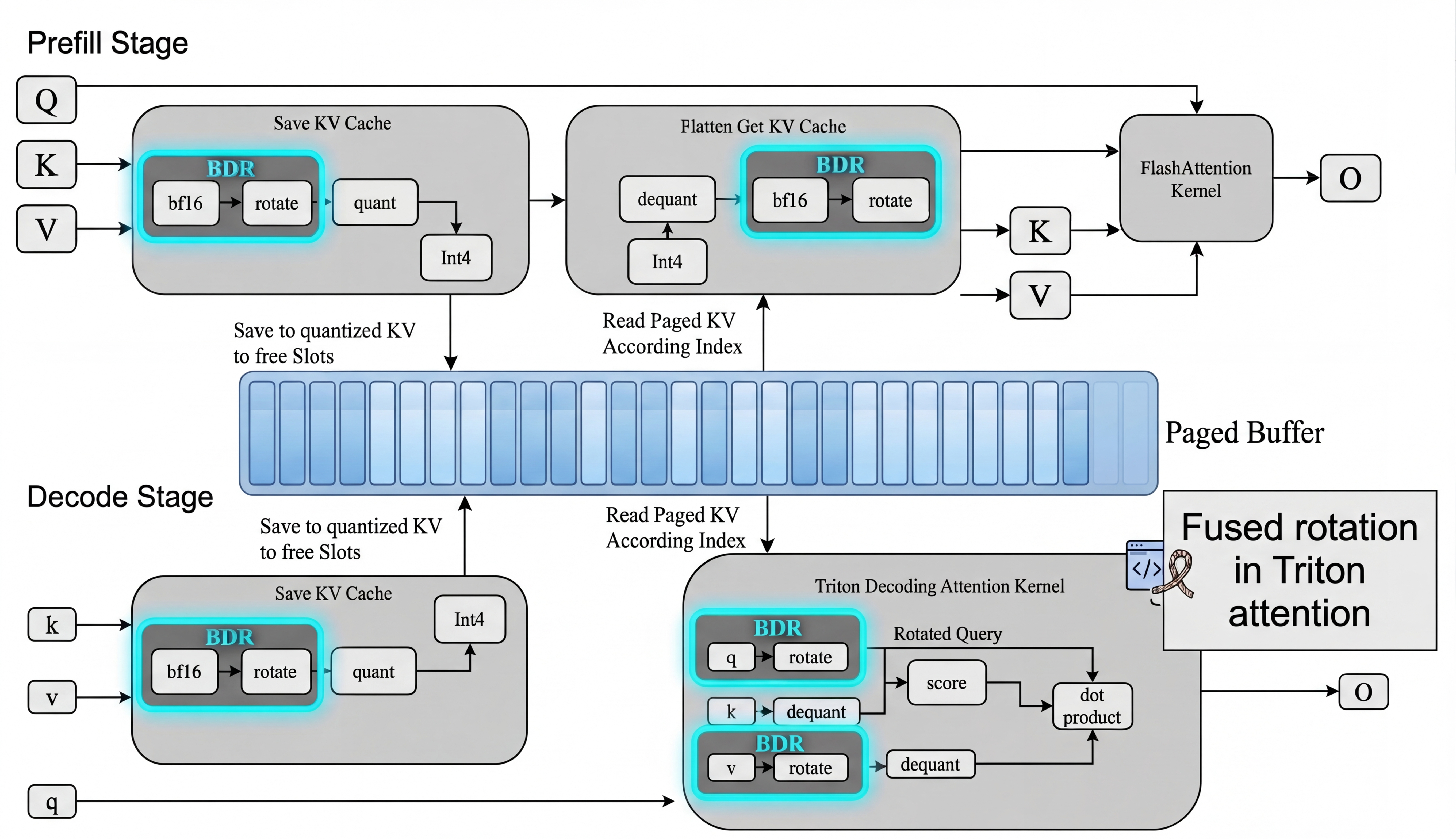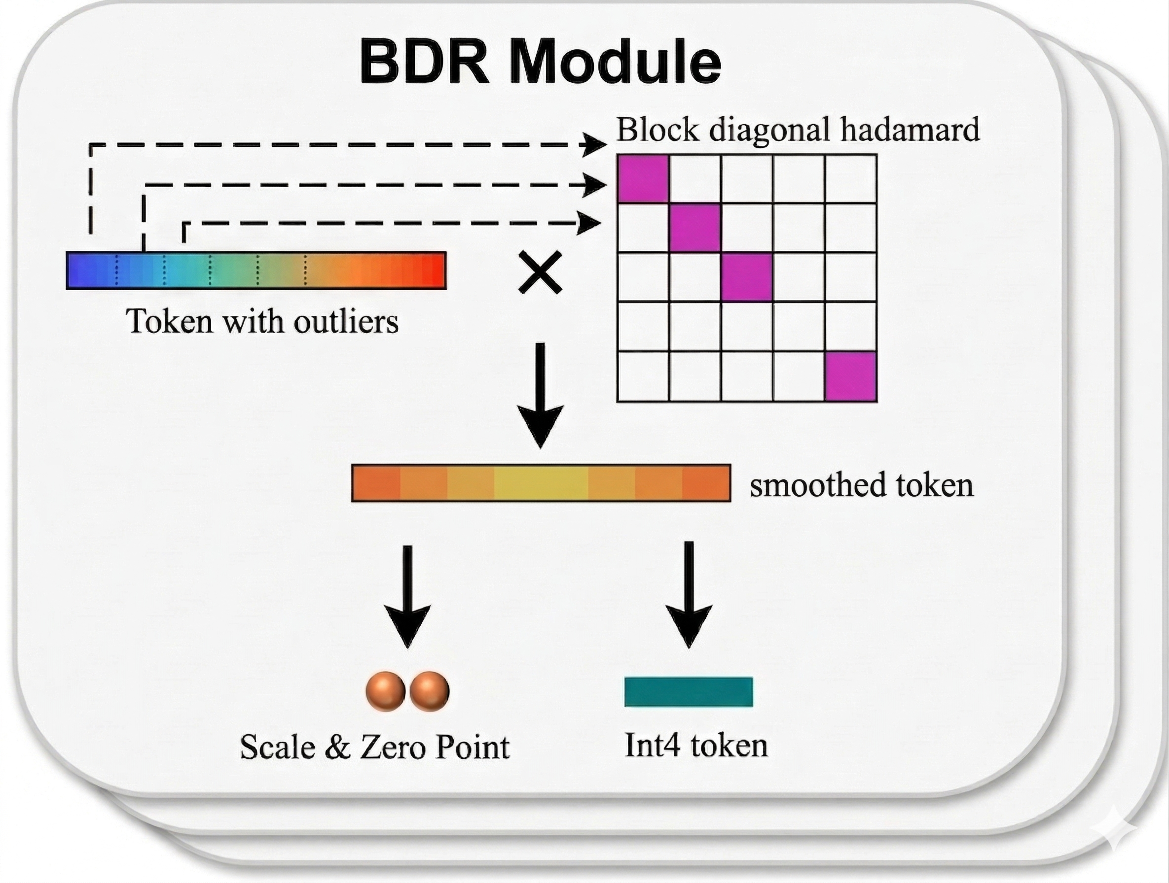</details> Figure 1: Overview of our system-aware INT4 KV-cache quantization framework (left) and rotate-quantize pipeline (right) for modern LLM serving. Table 1: Throughput on 2×H100 GPUs with 32 concurrent requests, each with an input length of 8192 tokens, output 1024 tokens. Here, TPS/User denotes tokens/s per user, and TPS/GPU denotes tokens/s per GPU. Acc is the mean computed over 5 tasks; each task is repeated 5 times. | | | Qwen3-4B-Thinking-2507 | Qwen3-8B | | | | | | --- | --- | --- | --- | --- | --- | --- | --- | | Method | Page Memory | TPS/User | TPS/GPU | Acc. | TPS/User | TPS/GPU | Acc. | | BF16 | 1 $×$ | 71.7 | 1030.5 | 75.64 | 61.9 | 859.1 | 70.84 | | INT4 | 4 $×$ | 86.7 | 1217.5 | 0 | 73.4 | 962.8 | 0 | | KMeans C=256 | 4 $×$ | 24.2 | 365.7 | 71.64 | 23.3 | 347.9 | 68.91 | | Hessian + BDR | 4 $×$ | 76.8 | 1051.0 | 65.52 | 66.3 | 887.2 | 70.59 | | BDR (Ours) | 4 $×$ | 88.3 | 1242.2 | 73.78 | 73.3 | 986.3 | 69.86 | Notes. BF16 denotes the full-precision KV cache, and INT4 denotes uniform 4-bit quantization. BDR- $k$ applies block-diagonal rotation with block size $k$ before INT4 quantization. K-means refers to vector quantization with $C$ centroids. Hessian+BDR applies block-diagonal rotation followed by Hessian-aware quantization. Naive INT4 fails to produce meaningful outputs. The five evaluation tasks are GPQA-Diamond, HumanEval, LiveCodeBench (v6), AIME25, and MATH500. All results are reported with a 32k sequence length in thinking mode. ### 1.1 Related Work As LLMs support increasingly long context windows, the key-value (KV) cache becomes a primary memory bottleneck. While architectural innovations such as grouped-query attention (Ainslie et al., 2023) and multi-head latent attention (Liu et al., 2024a) reduce the per-token footprint, absolute memory demand at long contexts remains a critical challenge, motivating a large body of work on post-training KV cache compression (LI et al., 2025). KV Cache Compression. Token eviction methods (Zhang et al., 2023; Xiao et al., 2023b) reduce cache size by discarding tokens deemed unimportant based on attention scores or recency. Scalar quantization methods (Liu et al., 2024c; Hooper et al., 2024; Kang et al., 2024; He et al., 2024; Xia et al., 2025) reduce the bit-width of KV activations, employing techniques such as per-channel key quantization, mixed-precision schemes, and outlier-aware encoding to achieve 2–4 bit compression with minimal quality loss. Beyond scalar approaches, vector quantization methods (Zhang et al., 2024; Li et al., 2025b; Zandieh et al., 2025) encode multiple dimensions of KV vectors jointly, exploiting inter-channel dependencies to push compression to 1–3 bits per channel while preserving model quality. Orthogonally, low-rank decomposition methods (Saxena et al., 2024; Chang et al., 2025) project keys and values into lower-rank subspaces, reducing both cache size and attention latency. Quantization Techniques. KV cache quantization methods draw on insights from broader LLM quantization research. A central challenge is activation outliers: LLM.int8() (Dettmers et al., 2022) isolates high-magnitude outlier dimensions into higher precision, while SmoothQuant (Xiao et al., 2023a) migrates quantization difficulty from activations to weights via per-channel scaling. For weight-only compression, Hessian-aware methods such as GPTQ (Frantar et al., 2022) and Happi (Kim et al., 2026) use second-order information to guide rounding and mixed-precision assignment. A separate line of work removes outliers through rotation: QuaRot (Ashkboos et al., 2024) applies randomized Hadamard transforms to produce near-uniform distributions, and SpinQuant (Liu et al., 2024b) learns optimal rotations on a Stiefel manifold, closing much of the accuracy gap at 4-bit quantization of weights, activations, and KV caches. At the extreme end, vector quantization methods such as QuIP# (Tseng et al., 2024a) and AQLM (Egiazarian et al., 2024) jointly encode groups of weight values using structured or learned codebooks, achieving strong results at 2–3 bits. ## 2 LLM Serving System and KV Compression Constraints A practical KV-cache quantization method must be evaluated not only by its offline compression ratio, but by whether it preserves throughput in a real serving stack. LLM serving imposes two non-negotiable constraints that invalidate some compression paradigms. Paged Memory Layouts: Modern systems (e.g., Kwon et al., 2023; Zheng et al., 2024) divide the KV cache into fixed-size, non-contiguous blocks to enable dynamic batching. This architectural reality breaks several approaches: - Token Eviction: Evicting “unimportant” tokens (e.g., Zhang et al., 2023) does not reduce the physical memory footprint unless an entire block is cleared, causing massive internal fragmentation. - Mixed-Precision: Methods using varying bit-widths (e.g., Xia et al., 2025) break the uniform layout required for efficient page table indexing. - Channel-Wise Scaling: Because tokens span non-contiguous blocks, computing shared scaling factors across channels (e.g., Liu et al., 2024c) requires highly inefficient cross-block memory access. <details> <summary>2604.19157v1/figures/throughput_gap.png Details</summary>  ### Visual Description ## Line Chart: Per-GPU Throughput vs. Batch Size ### Overview The chart compares the performance of different GPU configurations (SGLang BF16, HF Static FP16, HF Dynamic FP16, HF KIVI INT4, and Kitty-Pro) in terms of per-GPU throughput (tokens processed per second) across varying batch sizes (0–250). The y-axis represents throughput in tokens/second, while the x-axis represents batch size. Data points are plotted with distinct colors for each configuration, and trends indicate how throughput scales with batch size. --- ### Components/Axes - **Title**: "Per-GPU Throughput vs. Batch Size" - **X-axis (Batch Size)**: - Labels: 0, 50, 100, 150, 200, 250 - Scale: Linear increments of 50 - **Y-axis (Per-GPU Tokens/Second)**: - Labels: 0, 500, 1000, 1500, 2000, 2500, 3000 - Scale: Linear increments of 500 - **Legend**: - Position: Bottom-right corner - Entries: - **SGLang BF16**: Purple line with circular markers - **HF Static FP16**: Blue line with circular markers - **HF Dynamic FP16**: Orange line with circular markers - **HF KIVI INT4**: Green line with circular markers - **Kitty-Pro**: Red line with circular markers --- ### Detailed Analysis 1. **SGLang BF16 (Purple)**: - Starts at ~600 tokens/sec at batch size 1. - Rises sharply to ~1,700 tokens/sec at batch size 50. - Peaks at ~3,000 tokens/sec at batch size 100. - Declines slightly to ~2,900 tokens/sec at batch size 150. - Stabilizes near ~3,000 tokens/sec at batch sizes 200 and 250. 2. **Kitty-Pro (Red)**: - Begins at ~200 tokens/sec at batch size 1. - Increases steadily to ~1,500 tokens/sec at batch size 50. - Rises to ~1,700 tokens/sec at batch size 100. - Continues upward to ~1,900 tokens/sec at batch size 150. - Reaches ~2,100 tokens/sec at batch size 200. - Ends at ~2,200 tokens/sec at batch size 250. 3. **HF Static FP16 (Blue)**: - Starts at ~1,000 tokens/sec at batch size 1. - Drops to ~500 tokens/sec at batch size 50. - Further declines to ~300 tokens/sec at batch size 100. - Stabilizes at ~250 tokens/sec at batch sizes 150–250. 4. **HF Dynamic FP16 (Orange)**: - Begins at ~500 tokens/sec at batch size 1. - Peaks at ~600 tokens/sec at batch size 50. - Declines to ~400 tokens/sec at batch size 100. - Further drops to ~350 tokens/sec at batch size 150. - Ends at ~300 tokens/sec at batch size 250. 5. **HF KIVI INT4 (Green)**: - Remains flat at ~200–300 tokens/sec across all batch sizes. --- ### Key Observations - **SGLang BF16** dominates in throughput, especially at larger batch sizes (>100), maintaining near-peak performance. - **Kitty-Pro** shows consistent linear growth but lags behind SGLang BF16. - **HF Static FP16** underperforms significantly after batch size 1, suggesting inefficiency at scale. - **HF Dynamic FP16** and **HF KIVI INT4** exhibit minimal throughput, with HF KIVI INT4 being the least efficient. --- ### Interpretation The data highlights **SGLang BF16** as the most scalable and efficient configuration, achieving near-maximum throughput even at large batch sizes. **Kitty-Pro** demonstrates steady improvement but remains suboptimal compared to SGLang. The decline of **HF Static FP16** after small batch sizes suggests architectural limitations in handling larger workloads. **HF Dynamic FP16** and **HF KIVI INT4** underperform across all batch sizes, indicating potential inefficiencies in their design or implementation. These trends underscore the importance of configuration choice for optimizing GPU throughput in large-scale processing tasks. 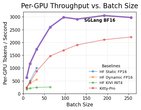</details> Figure 2: Qwen3-8B Per-GPU throughput vs. batch size. More complex methods (e.g., Kitty) do not match the performance of unquantized SGLang BF16. All non-SGLang-BF16 throughput numbers are measured with Hugging Face model.generate. which lacks continuous batching and PagedAttention, underestimating their performance. While methods like Kitty achieve strong offline compression, their complex memory access patterns make integration into optimized paged-memory engines highly non-trivial. As shown in Figure 2, when deployed in standard environments (e.g., Hugging Face generate) that lack PagedAttention and continuous batching, their end-to-end throughput falls massively behind even unquantized baselines running on highly optimized serving engines like SGLang. This highlights that quantization cannot be evaluated in a vacuum; if a compression method’s complexity precludes the use of standard system optimizations, it is a net negative for deployment. Attention Kernel: High-throughput decoding relies on FlashAttention style kernels that read directly from the paged buffer; therefore, dequantization must be fused in-kernel (Dao et al., 2022). For a decoding step: $o=softmax(qK^⊤/√{d})V$ where $q$ is a single query token and $(K,V)$ are read from the paged KV cache. This strict execution precludes: - Codebook Lookups: Vector quantization (e.g., Li et al., 2025a) requires global memory lookups during dequantization, increasing latency and bandwidth pressure. - Basis-Transforms: PCA/SVD methods require on-the-fly matrix-vector multiplications, inflating register pressure and destroying kernel tiling efficiency. - Strided Memory Access: Channel-wise quantization often forces channel-major memory access, destroying the memory coalescing required by GPU attention kernels. The Token-Wise Imperative: Taken together, these system constraints leave one most viable path. Token-wise quantization naturally operates independently on each token, avoids cross-block dependencies, and preserves coalesced memory access patterns. It is the only paradigm inherently compatible with paged layouts and fused kernels. Having established token-wise quantization as the necessary foundation, the remaining challenge is recovering the accuracy lost by naive INT4 implementations that we deconstruct in Section 3. ## 3 Method Comparison for Rotation Design Intuition To isolate the impact of different design choices under practical LLM serving constraints (e.g., paged KV-cache and fused kernels), we conduct a controlled token-wise comparison of four quantization strategies: naive INT4, vector quantization (KMeans) (Yang et al., 2026; Xi et al., 2026), Hessian-aware quantization (Kim et al., 2026; Zhou et al., 2026), and Hadamard rotation-based quantization. This section highlights our core design intuition; detailed derivations and extended evaluations are deferred to Appendix A. Token-Wise INT4 Quantization. We adopt an asymmetric token-wise INT4 scheme, quantizing each head vector $x_t,h$ using a per-token and per-head scale and zero-point. While highly system-friendly—reducing the KV-cache footprint from BF16 by $4×$ while preserving tensor layout—naive INT4 suffers from severe accuracy degradation. This is primarily driven by channel-wise range heterogeneity: high-magnitude outliers in specific channels artificially expand the quantization grid, leading to massive quantization errors across the rest of the vector (Hooper et al., 2024; Liu et al., 2024c; Zhang et al., 2024). Block-Diagonal Rotation Quantization. To remove data-driven calibration while mitigating channel-wise outliers, we apply an orthonormal transform $H$ to rotate the KV-cache (Ashkboos et al., 2024; Tseng et al., 2024b): $$ \tilde{K}=quant(KH), \tilde{V}=quant(VH). \tag{1} $$ As $H$ is orthogonal, it preserves the $\ell_2$ norm while redistributing energy across dimensions, reducing channel-wise variance and smoothing outliers—the main source of degradation under low-bit quantization (e.g., INT4). Attention can be computed directly in the rotated space or equivalently via $H^⊤$ , incurring no additional approximation error. In practice, we use randomized Hadamard transforms. However, full dense rotation over the full hidden dimension is costly. We therefore introduce block-diagonal rotation (BDR), decomposing the global transform into independent local rotations. Let $d_h$ be the head dimension. We partition each vector into blocks of size $h$ : $$ K=[K^(1),\dots,K^(d_h/h)], V=[V^(1),\dots,V^(d_h/h)], K^(i),V^(i)∈ℝ^h. \tag{1} $$ Each block is independently rotated and quantized: $\tilde{K}^(i)=quant(K^(i)H_h),\tilde{V}^(i)=quant(V^(i)H_h)$ where $H_h∈ℝ^h× h$ is a Hadamard matrix. This induces a block-diagonal transform $H_blk=diag(H_h,\dots,H_h)$ , approximating a full rotation at significantly lower cost and with better kernel efficiency. The block size $h$ controls the trade-off: larger $h$ improves cross-channel mixing and robustness, while smaller $h$ favors parallelism and kernel fusion. While smaller $h$ reduces per-rotation compute and improves kernel-level efficiency, we find that these gains do not consistently translate to end-to-end throughput improvements. This is because autoregressive decoding is primarily memory-bound, and rotation is not the dominant bottleneck. As a result, overly small blocks sacrifice quantization quality without delivering meaningful system-level gains. We will explain this in Section 4. Hessian-Aware Quantization. Following and inspired by prior Hessian- (or covariance-) aware quantization approaches (Kim et al., 2026; Zhou et al., 2026), we use decode-time query statistics to estimate attention-sensitive directions and derive a learned per-layer rotation for KV quantization. We instrument the serving engine to collect query vectors during offline calibration and, for each layer $\ell$ , form the second-moment matrix $M_\ell=\frac{1}{N_\ell}∑_i=1^N_\ellq_iq_i^⊤$ , which yields the score-error objective $L_\ell=δ k^⊤M_\ellδ k$ for key quantization error $δ k$ . We then take the resulting orthogonal eigenvector matrix $R_\ell$ as the learned per-layer rotation. At inference time, $R_\ell$ is composed with a Hadamard transform and applied to both $Q$ and $K$ , preserving full-precision attention logits while shifting quantization noise away from sensitive directions. Vector Quantization (KMeans). Vector quantization mitigates outlier degradation by mapping head vectors to a learned codebook of centroids. Here, $C$ denotes the number of centroids (codebook size) e.g., “KM w $C{=}256$ ” means KMeans with 256 clusters. By clustering similar activations rather than uniformly slicing the vector space, VQ recovers a substantial portion of the accuracy lost by scalar INT4. However, performance gains are not strictly monotonic with codebook size, highlighting a trade-off between representational capacity and the stability of the clustering algorithm during offline calibration. Detailed algorithmic description and residual-quantization formulation are provided in Appendix A. Table 2: Expanded comparison on Qwen3-4B-thinking-2507. Entries are $μ±σ$ over 5 runs. Mean is computed over available task means (all 5 tasks where available). | Method | GPQA | HumanE | LCB v6 | AIME | MATH | Mean | Drop | | --- | --- | --- | --- | --- | --- | --- | --- | | BF16 | 67.27 $±$ 1.80 | 94.05 $±$ 0.54 | 48.66 $±$ 2.20 | 74.67 $±$ 1.83 | 93.55 $±$ 0.33 | 75.64 | 0.00 | | INT4 | 0.00 $±$ 0.00 | 0.00 $±$ 0.00 | 0.00 $±$ 0.00 | 0.00 $±$ 0.00 | 0.00 $±$ 0.00 | 0.00 | -75.64 | | BDR-16 | 50.61 $±$ 2.35 | 56.20 $±$ 2.40 | 26.20 $±$ 2.85 | 54.67 $±$ 4.47 | 86.45 $±$ 0.61 | 54.83 | -20.81 | | BDR-64 | 63.13 $±$ 1.38 | 89.10 $±$ 0.39 | 46.66 $±$ 1.33 | 69.34 $±$ 4.35 | 93.23 $±$ 0.52 | 72.29 | -3.35 | | BDR-128 | 66.37 $±$ 2.19 | 89.78 $±$ 0.80 | 46.20 $±$ 1.94 | 70.00 $±$ 4.08 | 93.19 $±$ 0.51 | 73.11 | -2.53 | | BDR-128 (K) | 65.25 $±$ 2.12 | 90.49 $±$ 0.45 | 48.54 $±$ 1.65 | 71.33 $±$ 5.06 | 93.27 $±$ 0.36 | 73.78 | -1.86 | | Hessian+BDR-128 | 60.10 $±$ 2.03 | 84.27 $±$ 1.15 | 42.11 $±$ 1.96 | 53.33 $±$ 4.85 | 87.80 $±$ 0.42 | 65.52 | -10.41 | | KM w C=1 | 54.14 $±$ 1.53 | 81.76 $±$ 0.97 | 31.58 $±$ 3.15 | 18.67 $±$ 3.80 | 81.92 $±$ 0.70 | 53.61 | -22.03 | | KM w C=16 | 61.52 $±$ 2.43 | 91.00 $±$ 0.75 | 42.81 $±$ 2.53 | 64.00 $±$ 3.65 | 93.07 $±$ 0.30 | 70.48 | -5.16 | | KM w C=256 | 63.94 $±$ 0.58 | 91.85 $±$ 0.51 | 41.29 $±$ 1.73 | 68.00 $±$ 5.05 | 93.11 $±$ 0.11 | 71.64 | -4.00 | | KM w C=2048 | 60.71 $±$ 5.09 | 93.17 $±$ 0.49 | 43.16 $±$ 4.59 | 74.00 $±$ 6.41 | 93.03 $±$ 0.43 | 72.81 | -2.83 | | KM + BDR-128 | 65.25 $±$ 0.49 | 93.27 $±$ 0.63 | 47.25 $±$ 1.63 | 67.33 $±$ 2.5 | 93.63 $±$ 0.51 | 73.35 | -2.29 | Notes. BDR- $k$ refers to Block-Diagonal Rotation with block size $k$ , applied prior to INT4 quantization on Key and Value. BDR- $k$ (K) means we only apply rotation on K but not V before their quantization. Hessian+BDR-128 denotes applying BDR-128 followed by Hessian-based quantization. KM ( $C$ ) denotes K-means (vector quantization) with $C$ centroids. KM + BDR-128 applies BDR-128 on top of KM with $C=2048$ (the KM-only result for $C=2048$ is shown above; other variants are omitted due to space constraints). Table 3: Expanded comparison on Qwen3-8B and GLM-4.7 (358B). Entries are $μ±σ$ . | Method | GPQA | HumanE | LCB v6 | AIME | MATH | Mean | Drop | | --- | --- | --- | --- | --- | --- | --- | --- | | Qwen3-8B | | | | | | | | | BF16 | 56.67 $±$ 2.30 | 85.95 $±$ 1.01 | 49.01 $±$ 2.13 | 70.00 $±$ 3.33 | 92.59 $±$ 0.62 | 70.84 | – | | INT4 | 0.00 $±$ 0.00 | 0.00 $±$ 0.00 | 0.00 $±$ 0.00 | 0.00 $±$ 0.00 | 0.00 $±$ 0.00 | 0.00 | – | | BDR-16 | 54.85 $±$ 2.44 | 86.05 $±$ 0.80 | 47.13 $±$ 1.52 | 59.33 $±$ 5.96 | 92.06 $±$ 0.86 | 67.88 | -2.96 | | BDR-64 | 54.55 $±$ 1.55 | 87.59 $±$ 0.48 | 47.48 $±$ 2.16 | 64.00 $±$ 4.35 | 92.18 $±$ 0.64 | 69.16 | -1.68 | | BDR-64 (K) | 56.97 $±$ 0.83 | 86.59 $±$ 0.98 | 47.02 $±$ 1.58 | 66.00 $±$ 4.94 | 92.71 $±$ 0.37 | 69.86 | -0.99 | | BDR-128 | 54.85 $±$ 3.17 | 86.44 $±$ 0.42 | 47.95 $±$ 2.15 | 68.00 $±$ 2.98 | 92.63 $±$ 0.27 | 69.97 | -0.87 | | GLM-4.7 (358B) | | | | | | | | | BF16 | 73.23 $±$ 1.33 | 91.46 $±$ 0.65 | 49.12 $±$ 0.59 | 80.00 $±$ 3.33 | 95.66 $±$ 0.61 | 77.89 | – | | INT4 | 73.23 $±$ 1.34 | 91.14 $±$ 0.26 | 45.81 $±$ 1.79 | 80.00 $±$ 0.00 | 95.86 $±$ 0.31 | 77.21 | -0.68 | | BDR-16 | 72.90 $±$ 0.29 | 91.30 $±$ 0.63 | 50.68 $±$ 0.89 | 78.89 $±$ 1.92 | 95.46 $±$ 0.42 | 77.85 | -0.04 | | BDR-64 | 70.87 $±$ 1.54 | 92.11 $±$ 0.31 | 49.90 $±$ 1.79 | 81.11 $±$ 3.85 | 95.59 $±$ 0.35 | 77.92 | +0.03 | | BDR-128 | 73.74 $±$ 1.01 | 91.30 $±$ 0.92 | 50.49 $±$ 1.47 | 78.89 $±$ 1.92 | 95.32 $±$ 0.12 | 77.95 | +0.06 | ### 3.1 Empirical Results for Design Intuition We compare prior token-wise compatible KV-cache compression methods under a unified protocol on Qwen3-4B-thinking-2507 (Yang et al., 2025). Results are reported as $μ±σ$ over 5 runs on GPQA (Rein et al., 2024), HumanEval (Chen et al., 2021), LiveCodeBench v6 (Jain et al., 2024), AIME25 (math ai, 2025), and MATH500 (Hendrycks et al., 2021). We use $T=0.6$ , max sequence length 32k, and consistent decoding settings across methods. Rotation recovers most of the INT4 degradation. As shown in Table 2, naïve INT4 quantization is not viable on Qwen3-4B: all reported metrics collapse to nearly zero, indicating that low-bit KV-cache compression alone fails under realistic decoding conditions. Block-diagonal rotation, however, restores most of the lost accuracy. Increasing the block size from 16 to 64 yields a substantial improvement in mean score (54.83 $→$ 72.29), whereas increasing it further to 128 brings only a modest additional gain (73.11 versus 75.64 for BF16). These results suggest that moderate block-wise mixing is already sufficient to suppress the dominant channel-wise outliers induced by quantization. We further observe, consistent with Kitty (Xia et al., 2025), that applying rotation only to the key cache is sufficient in practice. Specifically, BDR-128 (K) in Table 2 and BDR-64 (K) in Table 3 achieve accuracy comparable to rotating both K and V. Section 4 complements this accuracy analysis with a runtime study, showing that a block size of 128 offers the best overall trade-off between quality and efficiency. Effect of quantization complexity. More complex quantization schemes do not substantially improve on this behavior. Vector quantization with KMeans benefits from larger codebooks, improving from 53.61 at $C{=}1$ to 72.81 at $C{=}2048$ , but still remains slightly below BDR-128. Hessian-aware quantization performs markedly worse than BDR-128 (63.23 versus 73.11), despite requiring extra calibration and offline complexity. Combining KMeans with rotation gives the strongest compressed result on Qwen3-4B (73.35), but the gain over BDR-128 alone is small. Overall, once rotation is applied, the remaining headroom is limited, and increasing quantization complexity appears to yield diminishing returns. For more combination results, see Table 8 and Table 9 in Appendix C. Scaling behavior across model sizes. Table 3 shows the same overall trend on Qwen3-8B: naïve INT4 again collapses, whereas rotation-based INT4 remains nearly lossless. In particular, BDR-128 achieves 69.97, only 0.87 points below the BF16 baseline of 70.84. GLM-4.7 exhibits a different pattern. Even naïve INT4 stays close to BF16 (77.21 vs. 77.89), suggesting that this model is intrinsically more robust to low-bit KV-cache quantization. Rotation still provides a further, albeit smaller, improvement. Taken together, these results suggest that the need for sophisticated compression is strongly model-dependent, but that block-diagonal rotation is the most reliable and system-compatible mechanism across settings. For sensitive models such as Qwen3, it turns an otherwise unusable INT4 baseline into a near-lossless one; for more robust models such as GLM-4.7, it preserves accuracy essentially for free. ## 4 Serving-Compatible KV Compression Method Having established that block-diagonal Hadamard rotation (BDR) recovers most of the accuracy lost by token-wise INT4 quantization, we now evaluate whether it preserves the serving efficiency critical to production LLM systems. A key observation is that kernel microbenchmarks and end-to-end serving performance need not align: plain INT4 can achieve higher isolated kernel bandwidth by avoiding rotation entirely, yet fused rotation introduces little measurable end-to-end penalty. This section explains why. ### 4.1 Kernel Optimization in Implementation Figure 1 illustrates how we integrate rotation into decoding. In a Triton decode kernel, each program processes one query and streams tiled key/value blocks for a single decoding step. Let $q$ denote the current query, and let $\tilde{K}_rot∈ℝ^S× h$ denote the INT4 key cache stored in the rotated space, where $S$ is the context length and $h$ is the rotation block size. The pre-softmax logits are computed as $(qH) dequant(\tilde{K}_rot)^⊤,$ with the Hadamard matrix $H$ . A key systems observation is that the cost of rotation is dominated less by arithmetic than by data movement. Applying rotation in a separate pass over the key cache would introduce extra kernel launches and additional global-memory traffic over a tensor of size $S× R$ , which is particularly undesirable during decoding since attention is already memory-bandwidth bound. To avoid this overhead, we fuse rotation directly into the decode attention kernel. Because the kernel already streams query, key, and value tiles, the query can be rotated on the fly and consumed immediately by the $qK$ dot-product loop, without materializing intermediate results. This design preserves the efficiency of the original INT4 decode path while avoiding an extra pass over KV-cache data. Table 4 reports the decode-time profiling breakdown. INT4-Fused-RotateK closely matches plain INT4 in total kernel time, showing that most rotation overhead is hidden once fused into the decode path. By contrast, the unfused implementation incurs additional overhead from separate rotation-related work. This confirms that the main systems objective is to eliminate extra passes over KV-cache data rather than to minimize the arithmetic cost of rotation in isolation. Detailed prefilling and decoding breakdowns are in Appendix B. Table 4: Decode kernel profiling breakdown by category for Qwen3-32B on 2 $×$ H100 with $tp=2$ at batch size 32 (single decoding step). Fused rotation closely matches plain INT4, while unfused rotation introduces additional overhead from extra auxiliary work. | Category | INT4 | INT4-Fused-RotateK | INT4-Unfused-RotateK | | | | | --- | --- | --- | --- | --- | --- | --- | | Time (ns) | Pct (%) | Time (ns) | Pct (%) | Time (ns) | Pct (%) | | | MatMul | 176,800 | 33.16 | 176,703 | 33.35 | 175,391 | 32.44 | | Attention | 326,842 | 61.30 | 322,880 | 60.93 | 322,816 | 59.71 | | Comm | 11,200 | 2.10 | 11,519 | 2.17 | 14,496 | 2.68 | | _quantized_set_kv_int4_kernel | 5,504 | 1.03 | 6,112 | 1.15 | 5,504 | 1.02 | | Norm_Act_RoPE | 12,800 | 2.40 | 12,704 | 2.40 | 13,026 | 2.41 | | Outside_Kernel_Rotation | – | – | – | – | 9,376 | 1.73 | | TOTAL | 533,146 | 100.00 | 529,918 | 100.00 | 540,609 | 100.00 | Notes. MatMul: GEMM kernels; Attention: decode-attention kernels; Comm: cross_device_reduce_*; _quantized_set_kv_int4_kernel: INT4 KV-cache write (including fused Hadamard + KV write); Norm_Act_RoPE: RMSNorm, activation, RoPE, and QK-norm; Outside_Kernel_Rotation: unfused rotation overhead. ### 4.2 From Kernel Throughput to End-to-End Latency <details> <summary>2604.19157v1/x1.png Details</summary>  ### Visual Description ## Bar Chart: KV int4 + fused Hxint4 throughput vs T (H100, D=128, H=8) ### Overview The chart compares throughput (GB/s) across different token lengths (T) for five configurations: "int4 (plain)" (gray), "order 16" (red), "order 32" (orange), "order 64" (light orange), and "order 128" (yellow). Token lengths range from 32 to 16K, with throughput values plotted on a logarithmic y-axis (10¹ to 10⁴ GB/s). --- ### Components/Axes - **X-axis (Token length T)**: 32, 256, 1K, 4K, 8K, 16K (logarithmic spacing). - **Y-axis (Throughput)**: Logarithmic scale (10¹ to 10⁴ GB/s). - **Legend**: - Gray: "int4 (plain)" - Red: "order 16" - Orange: "order 32" - Light orange: "order 64" - Yellow: "order 128" - **Bar Groups**: Each token length has five bars (one per configuration), positioned side-by-side. --- ### Detailed Analysis #### Token Length = 32 - **int4 (plain)**: 9 GB/s (gray) - **order 16**: 7 GB/s (red) - **order 32**: 7 GB/s (orange) - **order 64**: 7 GB/s (light orange) - **order 128**: 7 GB/s (yellow) #### Token Length = 256 - **int4 (plain)**: 73 GB/s (gray) - **order 16**: 50 GB/s (red) - **order 32**: 54 GB/s (orange) - **order 64**: 55 GB/s (light orange) - **order 128**: 52 GB/s (yellow) #### Token Length = 1K - **int4 (plain)**: 270 GB/s (gray) - **order 16**: 208 GB/s (red) - **order 32**: 209 GB/s (orange) - **order 64**: 219 GB/s (light orange) - **order 128**: 219 GB/s (yellow) #### Token Length = 4K - **int4 (plain)**: 882 GB/s (gray) - **order 16**: 694 GB/s (red) - **order 32**: 710 GB/s (orange) - **order 64**: 698 GB/s (light orange) - **order 128**: 662 GB/s (yellow) #### Token Length = 8K - **int4 (plain)**: 1,085 GB/s (gray) - **order 16**: 898 GB/s (red) - **order 32**: 877 GB/s (orange) - **order 64**: 855 GB/s (light orange) - **order 128**: 834 GB/s (yellow) #### Token Length = 16K - **int4 (plain)**: 1,301 GB/s (gray) - **order 16**: 1,065 GB/s (red) - **order 32**: 1,035 GB/s (orange) - **order 64**: 1,015 GB/s (light orange) - **order 128**: 980 GB/s (yellow) --- ### Key Observations 1. **int4 (plain) dominates**: The gray bars (int4 plain) consistently show the highest throughput across all token lengths, with values up to 1,301 GB/s at 16K tokens. 2. **Order 128 underperforms**: The yellow bars (order 128) have the lowest throughput, particularly at larger token lengths (e.g., 980 GB/s at 16K vs. 1,301 GB/s for int4). 3. **Throughput scaling**: All configurations show exponential growth with token length, but int4 scales most effectively. 4. **Order 16 vs. order 32**: At 256 tokens, order 16 (50 GB/s) underperforms order 32 (54 GB/s), but this reverses at 1K tokens (208 vs. 209 GB/s). --- ### Interpretation - **Efficiency of int4**: The "int4 (plain)" configuration likely avoids overhead from fused operations, making it the most efficient. Fused Hxint4 (other orders) introduces diminishing returns as token length increases. - **Order 128 bottleneck**: The yellow bars (order 128) suggest that higher-order configurations may face resource contention or algorithmic inefficiencies, reducing throughput despite increased token length. - **Logarithmic scaling**: The y-axis emphasizes exponential growth, particularly in the 16K range, where int4 reaches ~1.3k GB/s, while order 128 plateaus near 1k GB/s. - **Anomalies**: The slight dip in order 16 performance at 256 tokens (50 GB/s) compared to order 32 (54 GB/s) may indicate configuration-specific optimizations or trade-offs. --- ### Spatial Grounding - **Legend**: Top-left corner, aligned with bar colors. - **X-axis labels**: Centered below each token length group. - **Y-axis**: Left-aligned, with logarithmic ticks (10¹, 10², ..., 10⁴). - **Bar placement**: Each token length group has five bars, ordered left-to-right per legend (gray → yellow). --- ### Content Details - **Values**: Extracted from bar heights, with approximate uncertainty (±5–10% based on visual estimation). - **Trends**: All configurations show increasing throughput with token length, but int4 maintains a consistent lead. - **Color consistency**: Legend colors match bar colors exactly (e.g., red = order 16). --- ### Final Notes The chart highlights the trade-off between configuration complexity (order) and throughput efficiency. While fused Hxint4 configurations (orders 16–128) improve with token length, they cannot match the plain int4 setup, suggesting that simplicity in design may be critical for high-throughput systems. 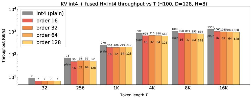</details> Figure 3: Effective bandwidth (GB/s) on H100 for the fused block rotate–quantize–save KV-cache kernel, grouped by sequence length, with $HeadDimension{=}128$ and $Heads{=}8$ . Within each group, bars correspond to different Hadamard block orders $h∈\{16,32,64,128\}$ . As expected, Figure 3 shows that plain INT4 achieves the highest isolated kernel bandwidth since it avoids rotation entirely. Consequently, fused rotation is slightly slower in this microbenchmark. However, this gap should not be overinterpreted: it reflects only the local KV-cache kernel cost, not the serving stack. In end-to-end serving, latency depends not only on the decode kernel, but also on scheduling, memory management, communication, and other runtime overheads (as displayed in Table 4). Moreover, the rotated INT4 path accounts for only a fraction of total decode latency, and the incremental cost of rotation is smaller still once integrated into the normal query-key streaming loop. As a result, the kernel-level advantage of INT4 largely disappears in end-to-end latency. 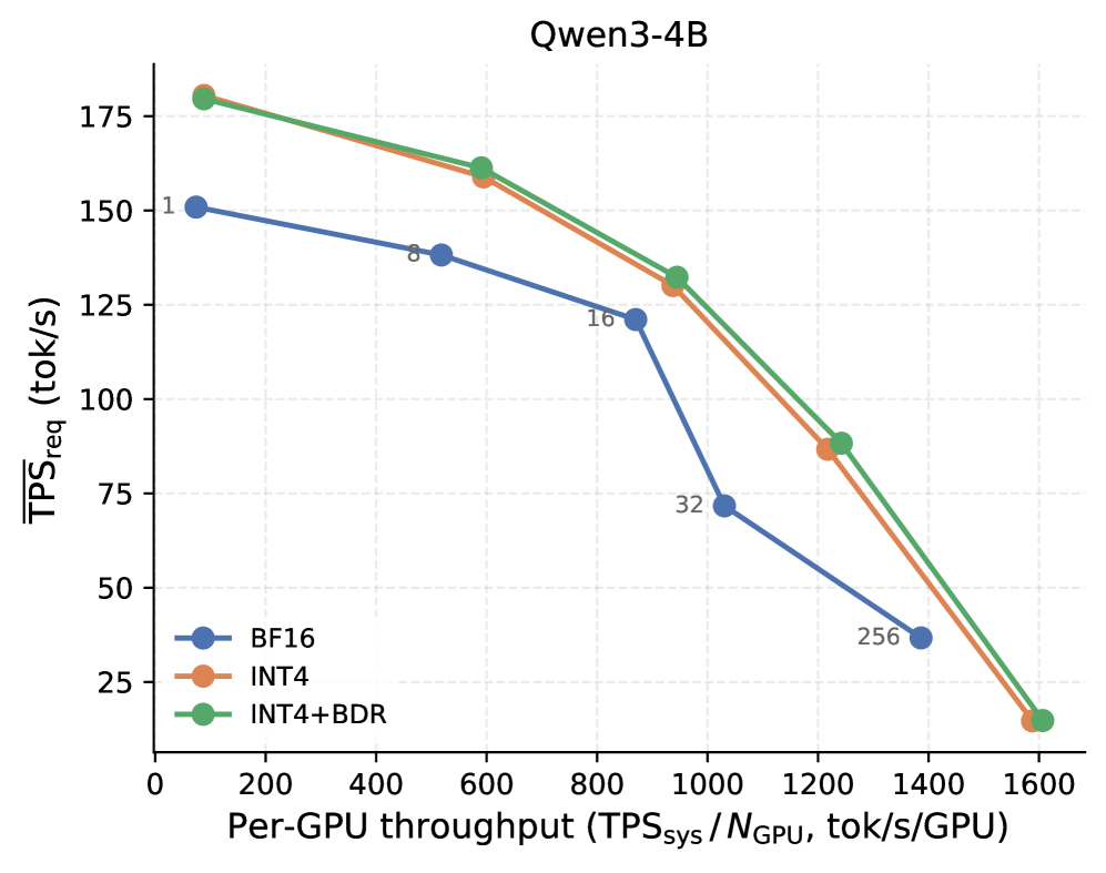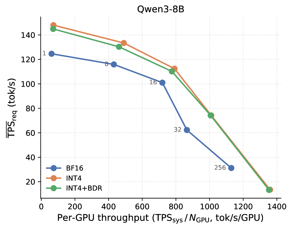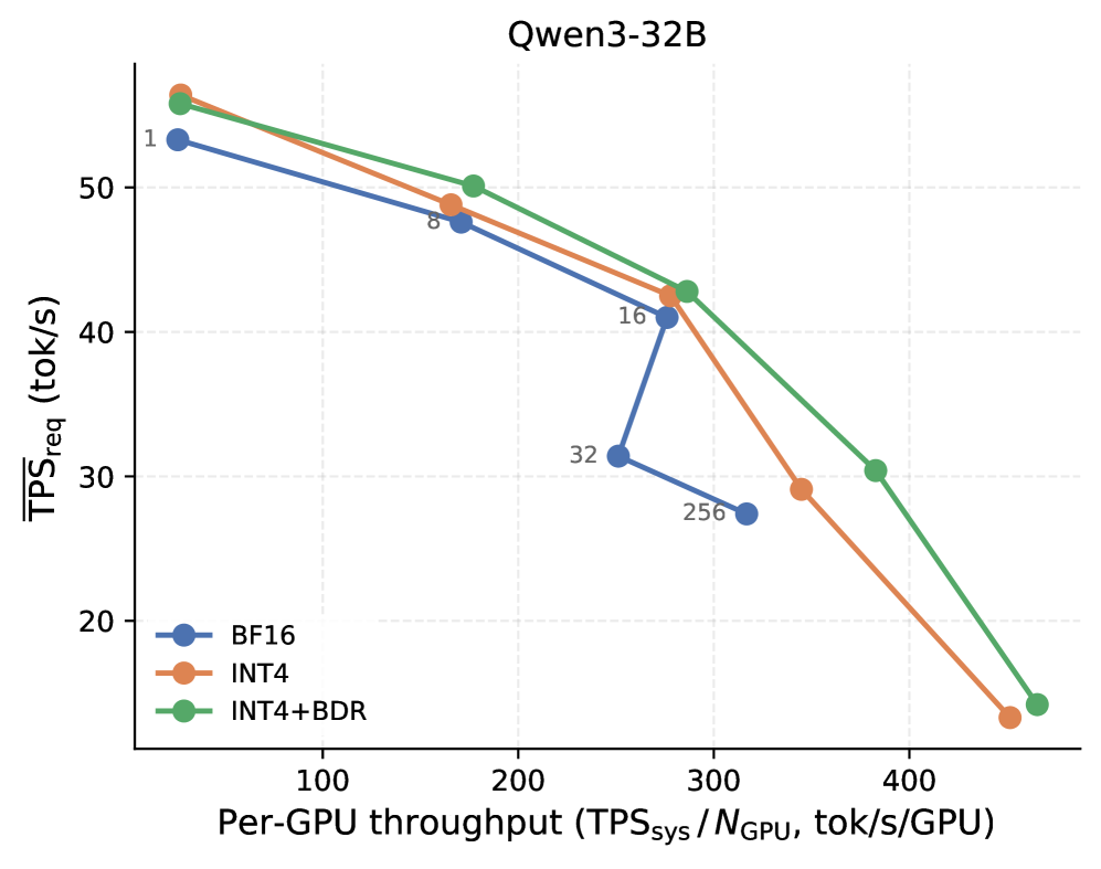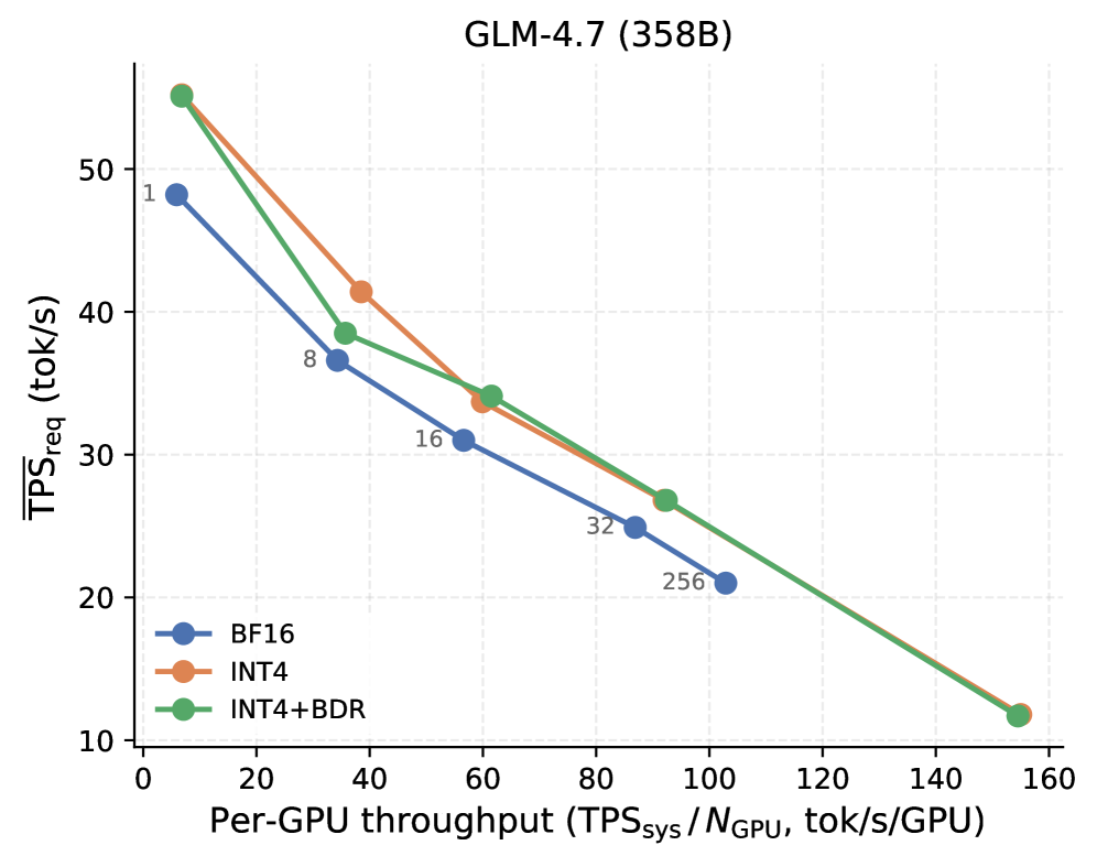This interpretation is consistent with the serving results in Figure 4. Across all four workloads, spanning model sizes from Qwen3-4B and Qwen3-8B to Qwen3-32B and GLM-4.7 (358B), INT4 with fused BDR (green curves) consistently matches plain INT4 while outperforming BF16 across most operating regimes. This shows that the small kernel-level advantage of plain INT4 does not translate into a meaningful end-to-end gap. We further compare end-to-end throughput against k-means and Hessian-based methods and also include additional comparisons between our INT4 method and Kitty. The complete results are shown in Figure 7 and Figure 8 in Appendix D. Overall, rotation preserves the benefits of INT4 while substantially improving model quality, highlighting that end-to-end performance matters more than isolated kernel microbenchmarks. <details> <summary>2604.19157v1/x2.png Details</summary>  ### Visual Description ## Line Chart: Qwen3-4B Performance Comparison ### Overview The chart compares the performance of three quantization methods (BF16, INT4, INT4+BDR) for the Qwen3-4B model, plotting **TPS_req (tokens/second)** against **Per-GPU throughput (TPS_sys/N_GPU, tok/s/GPU)**. All three lines show a downward trend, indicating decreasing TPS_req as throughput increases. ### Components/Axes - **X-axis**: Per-GPU throughput (TPS_sys/N_GPU, tok/s/GPU) - Markers: 0, 200, 400, 600, 800, 1000, 1200, 1400, 1600 - **Y-axis**: TPS_req (tok/s) - Markers: 25, 50, 75, 100, 125, 150, 175 - **Legend**: - **BF16** (blue line with circle markers) - **INT4** (orange line with circle markers) - **INT4+BDR** (green line with circle markers) - Positioned in the bottom-left corner. ### Detailed Analysis 1. **BF16 (Blue Line)** - Starts at **150 tok/s** at x=0. - Gradual decline to **140 tok/s** at x=400. - Further drops to **130 tok/s** at x=800. - Sharp decline to **70 tok/s** at x=1000. - Final drop to **30 tok/s** at x=1400. 2. **INT4 (Orange Line)** - Starts at **180 tok/s** at x=0. - Declines to **160 tok/s** at x=400. - Further drops to **140 tok/s** at x=800. - Sharp decline to **130 tok/s** at x=1000. - Final drop to **85 tok/s** at x=1200. - Ends at **15 tok/s** at x=1600. 3. **INT4+BDR (Green Line)** - Starts at **180 tok/s** at x=0. - Declines to **165 tok/s** at x=400. - Further drops to **145 tok/s** at x=800. - Sharp decline to **135 tok/s** at x=1000. - Further drops to **90 tok/s** at x=1200. - Ends at **15 tok/s** at x=1600. ### Key Observations - **INT4+BDR** consistently outperforms **INT4** and **BF16** across all throughput ranges, maintaining lower TPS_req. - **BF16** shows the steepest decline after x=1000, suggesting reduced efficiency at higher throughputs. - All methods converge to **~15 tok/s** at x=1600, indicating a performance floor. - **INT4+BDR** retains ~10-15 tok/s advantage over **INT4** and ~30-40 tok/s advantage over **BF16** at mid-range throughputs (x=400–1000). ### Interpretation The chart demonstrates that **INT4+BDR** offers the best trade-off between throughput and token processing efficiency, likely due to optimized quantization techniques. **BF16**, while simpler, becomes less efficient at higher throughputs, possibly due to higher memory or computational overhead. The convergence at x=1600 suggests diminishing returns for all methods at extreme throughputs. This data could guide model deployment decisions, favoring INT4+BDR for latency-sensitive applications. </details> <details> <summary>2604.19157v1/x3.png Details</summary>  ### Visual Description ## Line Chart: Qwen3-8B Performance Analysis ### Overview The chart compares the relationship between per-GPU throughput (x-axis) and required tokens per second (y-axis) for three configurations of the Qwen3-8B model: BF16, INT4, and INT4+BDR. All three lines show a downward trend, indicating that higher per-GPU throughput reduces the required TPS. ### Components/Axes - **X-axis**: Per-GPU throughput (TPS_sys / N_GPU, tok/s/GPU) - Scale: 0 to 1400 (logarithmic spacing implied by axis markers) - Labels: 1, 8, 16, 32, 256, 1000, 1400 - **Y-axis**: TPS_req (tok/s) - Scale: 0 to 160 (linear increments of 20) - Labels: 20, 40, 60, 80, 100, 120, 140 - **Legend**: - **BF16**: Blue line with circular markers - **INT4**: Orange line with circular markers - **INT4+BDR**: Green line with circular markers - **Placement**: Legend is positioned in the bottom-left corner, aligned with the x-axis. ### Detailed Analysis 1. **BF16 (Blue Line)** - Data Points: - (1, 120) - (8, 110) - (16, 100) - (32, 60) - (256, 30) - Trend: Gradual decline with a steep drop between 16 and 32. 2. **INT4 (Orange Line)** - Data Points: - (1, 150) - (8, 135) - (16, 120) - (32, 90) - (256, 45) - (1000, 75) - (1400, 15) - Trend: Steeper initial decline than BF16, with a sharp drop at 1000 and 1400. 3. **INT4+BDR (Green Line)** - Data Points: - (1, 145) - (8, 130) - (16, 115) - (32, 85) - (256, 40) - (1000, 70) - (1400, 15) - Trend: Similar to INT4 but slightly lower TPS_req across most ranges. ### Key Observations - **Convergence at High Throughput**: All three lines converge near (1400, 15), suggesting diminishing returns in efficiency gains beyond this point. - **INT4 vs. BF16**: INT4 consistently outperforms BF16 at higher throughputs (e.g., 256: 45 vs. 30 tok/s). - **INT4+BDR Efficiency**: Outperforms both BF16 and INT4 at most throughput levels, with the largest gap at 1000 (70 vs. 75 tok/s for INT4). - **BF16 Plateau**: BF16’s TPS_req stabilizes at 30 tok/s after 256 throughput, while INT4 and INT4+BDR continue declining. ### Interpretation The chart demonstrates that **INT4+BDR** achieves the highest efficiency (lowest TPS_req) across most throughput ranges, followed by INT4 and then BF16. The convergence at 1400 throughput suggests that all configurations reach a similar performance ceiling, likely due to hardware or algorithmic limitations. - **Practical Implications**: - For high-throughput scenarios (>256), INT4+BDR is optimal. - BF16 may be preferable for low-throughput applications where memory or precision is prioritized over speed. - **Anomalies**: - The sharp drop in INT4 and INT4+BDR at 1000 throughput (from 45 to 75 and 40 to 70, respectively) may indicate a transition between hardware layers or optimization thresholds. - BF16’s plateau at 30 tok/s could reflect fixed memory constraints or quantization limits. This analysis highlights trade-offs between precision (BF16), quantization (INT4), and memory optimization (INT4+BDR) in deploying large language models like Qwen3-8B. </details> <details> <summary>2604.19157v1/x4.png Details</summary>  ### Visual Description ## Line Chart: Owen3-32B Performance Analysis ### Overview The chart compares the performance of three model configurations (BF16, INT4, INT4+BDR) across varying Per-GPU throughput levels, measured in tokens per second (tok/s). The y-axis represents required TPS (TPS_req), while the x-axis shows Per-GPU throughput (TPS_sys/N_GPU, tok/s/GPU). All three lines exhibit downward trends, indicating improved efficiency as throughput increases. ### Components/Axes - **X-axis**: Per-GPU throughput (TPS_sys/N_GPU, tok/s/GPU) Scale: 100 → 400 (logarithmic spacing implied by axis markers) - **Y-axis**: TPS_req (tok/s) Scale: 20 → 50 (linear increments) - **Legend**: - Blue circles: BF16 - Orange circles: INT4 - Green circles: INT4+BDR Positioned in the bottom-left corner. ### Detailed Analysis #### BF16 (Blue Line) - Data points: (100, 50), (150, 48), (200, 45), (250, 42), (300, 32), (350, 25) - Trend: Gradual decline with minimal curvature. #### INT4 (Orange Line) - Data points: (100, 55), (150, 52), (200, 49), (250, 45), (300, 42), (350, 30), (400, 15) - Trend: Steeper decline after 300 throughput, with a sharp drop at 400. #### INT4+BDR (Green Line) - Data points: (100, 53), (150, 50), (200, 47), (250, 43), (300, 42), (350, 30), (400, 15) - Trend: Similar to INT4 but consistently outperforms BF16 across all throughputs. ### Key Observations 1. **Performance Scaling**: All configurations show improved efficiency (lower TPS_req) as Per-GPU throughput increases. 2. **INT4 vs. BF16**: INT4 outperforms BF16 by 3–5 TPS_req at equivalent throughputs, with the gap widening at higher throughputs (e.g., 15 TPS_req difference at 400). 3. **INT4+BDR Advantage**: Maintains a 1–2 TPS_req edge over INT4 across most throughputs, suggesting BDR optimization provides marginal gains. 4. **Threshold Behavior**: INT4 and INT4+BDR exhibit a steeper performance drop after 300 throughput, potentially indicating hardware/software bottlenecks. ### Interpretation The data demonstrates that model quantization (INT4) and BDR optimizations significantly improve throughput efficiency compared to BF16. However, the sharp decline in INT4/INT4+BDR performance beyond 300 throughput suggests diminishing returns or resource contention at higher loads. This implies that while INT4+BDR is optimal for high-throughput scenarios, workload distribution strategies may need adjustment to avoid performance cliffs. The consistent gap between BF16 and the other configurations highlights the trade-offs between precision (BF16) and efficiency (INT4 variants) in large language model deployment. </details> <details> <summary>2604.19157v1/x5.png Details</summary>  ### Visual Description ## Line Chart: GLM-4.7 (358B) Performance Analysis ### Overview The chart compares the relationship between **per-GPU throughput** (x-axis) and **required tokens per second (TPS_req)** (y-axis) for three configurations of the GLM-4.7 (358B) model: BF16, INT4, and INT4+BDR. All three lines show a decreasing trend, indicating that higher throughput reduces the required TPS_req. ### Components/Axes - **X-axis**: "Per-GPU throughput (TPS_sys/N_GPU, tok/s/GPU)" - Scale: 0 to 160 (logarithmic spacing implied by gridlines). - Key markers: 1, 8, 16, 32, 80, 100, 160. - **Y-axis**: "TPS_req (tok/s)" - Scale: 10 to 50 (linear increments of 10). - **Legend**: Bottom-left corner, with color-coded labels: - Blue: BF16 - Orange: INT4 - Green: INT4+BDR ### Detailed Analysis #### Data Points and Trends 1. **BF16 (Blue Line)** - Starts at **~48 TPS_req** at 1 tok/s/GPU. - Drops sharply to **~38 TPS_req** at 8 tok/s/GPU. - Continues declining to **~31 TPS_req** at 16 tok/s/GPU. - Further reduces to **~26 TPS_req** at 32 tok/s/GPU. - Ends at **~20 TPS_req** at 100 tok/s/GPU. - **Trend**: Steepest initial decline, then gradual flattening. 2. **INT4 (Orange Line)** - Starts at **~55 TPS_req** at 1 tok/s/GPU. - Drops to **~41 TPS_req** at 40 tok/s/GPU. - Reduces to **~33 TPS_req** at 60 tok/s/GPU. - Further declines to **~28 TPS_req** at 80 tok/s/GPU. - Ends at **~25 TPS_req** at 100 tok/s/GPU. - **Trend**: Consistent linear decline, slower than BF16. 3. **INT4+BDR (Green Line)** - Starts at **~55 TPS_req** at 1 tok/s/GPU (same as INT4). - Drops to **~38 TPS_req** at 40 tok/s/GPU. - Reduces to **~33 TPS_req** at 60 tok/s/GPU. - Further declines to **~27 TPS_req** at 80 tok/s/GPU. - Ends at **~25 TPS_req** at 100 tok/s/GPU. - **Trend**: Similar to INT4 but slightly lower TPS_req at higher throughputs. ### Key Observations - All configurations show **inverse proportionality**: Higher throughput reduces TPS_req. - **BF16** requires the highest TPS_req initially but converges with INT4+BDR at 100 tok/s/GPU. - **INT4+BDR** outperforms INT4 at 80 and 100 tok/s/GPU, suggesting BDR improves efficiency. - At 160 tok/s/GPU, all lines extrapolate to **~12–15 TPS_req**, though data is not explicitly plotted. ### Interpretation The chart demonstrates that **model precision and optimization techniques** (e.g., BDR) significantly impact throughput efficiency. - **BF16** (likely 16-bit floating-point) has higher computational overhead, requiring more TPS_req even at lower throughputs. - **INT4** (4-bit integer) and **INT4+BDR** (with BDR, possibly batch data reuse or quantization) achieve better scalability. - The convergence of INT4 and INT4+BDR at high throughputs implies BDR mitigates precision-related bottlenecks. - The steep decline in BF16 suggests it is less optimized for high-throughput scenarios compared to INT4 variants. This analysis highlights trade-offs between model precision, optimization methods, and system performance in large language models like GLM-4.7. </details> Figure 4: $\overline{TPS}_req$ versus per-GPU throughput ( $TPS_sys/N_GPU$ ). The top row shows Qwen3-4B and Qwen3-8B; the bottom row shows Qwen3-32B and GLM-4.7 (358B). INT4 + R128 consistently matches or slightly exceeds plain INT4 and outperforms BF16 across most operating regimes, showing that rotation preserves INT4 efficiency while improving model quality. ## 5 Conclusion This paper asks a simple question: under real serving constraints, what is the minimal INT4 KV-cache quantization method that actually works? Our answer is equally simple: token-wise quantization plus block-diagonal Hadamard rotation. Across models and workloads, this design recovers most of the accuracy lost by naive INT4 while preserving essentially the same serving behavior. More complex alternatives, such as Hessian-aware or vector-quantized variants, add calibration or implementation complexity but yield only marginal gains once serving compatibility is taken into account. Our results also highlight a broader systems lesson. Kernel microbenchmarks alone can be misleading: a local kernel advantage does not necessarily translate into a meaningful end-to-end serving gain. What matters in practice is preserving the memory-capacity and throughput benefits of INT4 without disrupting the serving stack. By fusing rotation into the KV-cache path, we achieve exactly this, showing that effective KV-cache compression is ultimately a systems co-design problem rather than a purely quantization-driven one. ## References - Ainslie et al. (2023) Joshua Ainslie, James Lee-Thorp, Michiel De Jong, Yury Zemlyanskiy, Federico Lebrón, and Sumit Sanghai. Gqa: Training generalized multi-query transformer models from multi-head checkpoints. In Proceedings of the 2023 Conference on Empirical Methods in Natural Language Processing, pp. 4895–4901, 2023. - Ashkboos et al. (2024) Saleh Ashkboos, Amirkeivan Mohtashami, Maximilian L. Croci, Bo Li, Pashmina Cameron, Martin Jaggi, Dan Alistarh, Torsten Hoefler, and James Hensman. Quarot: Outlier-free 4-bit inference in rotated LLMs. In The Thirty-eighth Annual Conference on Neural Information Processing Systems, 2024. URL https://openreview.net/forum?id=dfqsW38v1X. - Belcak et al. (2025) Peter Belcak, Greg Heinrich, Shizhe Diao, Yonggan Fu, Xin Dong, Saurav Muralidharan, Yingyan Celine Lin, and Pavlo Molchanov. Small language models are the future of agentic ai. arXiv preprint arXiv:2506.02153, 2025. - Chang et al. (2025) Chi-Chih Chang, Wei-Cheng Lin, Chien-Yu Lin, Chong-Yan Chen, Yu-Fang Hu, Pei-Shuo Wang, Ning-Chi Huang, Luis Ceze, Mohamed S. Abdelfattah, and Kai-Chiang Wu. Palu: KV-cache compression with low-rank projection. In The Thirteenth International Conference on Learning Representations, 2025. URL https://openreview.net/forum?id=LWMS4pk2vK. - Chen et al. (2021) Mark Chen, Jerry Tworek, Heewoo Jun, Qiming Yuan, Henrique Ponde De Oliveira Pinto, Jared Kaplan, Harri Edwards, Yuri Burda, Nicholas Joseph, Greg Brockman, et al. Evaluating large language models trained on code. arXiv preprint arXiv:2107.03374, 2021. - Comanici et al. (2025) Gheorghe Comanici, Eric Bieber, Mike Schaekermann, Ice Pasupat, Noveen Sachdeva, Inderjit Dhillon, Marcel Blistein, Ori Ram, Dan Zhang, Evan Rosen, et al. Gemini 2.5: Pushing the frontier with advanced reasoning, multimodality, long context, and next generation agentic capabilities. arXiv preprint arXiv:2507.06261, 2025. - Dao et al. (2022) Tri Dao, Dan Fu, Stefano Ermon, Atri Rudra, and Christopher Ré. Flashattention: Fast and memory-efficient exact attention with io-awareness. Advances in neural information processing systems, 35:16344–16359, 2022. - Dettmers et al. (2022) Tim Dettmers, Mike Lewis, Younes Belkada, and Luke Zettlemoyer. Gpt3. int8 (): 8-bit matrix multiplication for transformers at scale. Advances in neural information processing systems, 35:30318–30332, 2022. - Egiazarian et al. (2024) Vage Egiazarian, Andrei Panferov, Denis Kuznedelev, Elias Frantar, Artem Babenko, and Dan Alistarh. Extreme compression of large language models via additive quantization. arXiv preprint arXiv:2401.06118, 2024. - Frantar et al. (2022) Elias Frantar, Saleh Ashkboos, Torsten Hoefler, and Dan Alistarh. Gptq: Accurate post-training quantization for generative pre-trained transformers. arXiv preprint arXiv:2210.17323, 2022. - He et al. (2024) Yefei He, Luoming Zhang, Weijia Wu, Jing Liu, Hong Zhou, and Bohan Zhuang. Zipcache: Accurate and efficient kv cache quantization with salient token identification. Advances in Neural Information Processing Systems, 37:68287–68307, 2024. - Hendrycks et al. (2021) Dan Hendrycks, Collin Burns, Saurav Kadavath, Akul Arora, Steven Basart, Eric Tang, Dawn Song, and Jacob Steinhardt. Measuring mathematical problem solving with the math dataset. arXiv preprint arXiv:2103.03874, 2021. - Hooper et al. (2024) Coleman Richard Charles Hooper, Sehoon Kim, Hiva Mohammadzadeh, Michael W. Mahoney, Sophia Shao, Kurt Keutzer, and Amir Gholami. KVQuant: Towards 10 million context length LLM inference with KV cache quantization. In The Thirty-eighth Annual Conference on Neural Information Processing Systems, 2024. URL https://openreview.net/forum?id=0LXotew9Du. - Jain et al. (2024) Naman Jain, King Han, Alex Gu, Wen-Ding Li, Fanjia Yan, Tianjun Zhang, Sida Wang, Armando Solar-Lezama, Koushik Sen, and Ion Stoica. Livecodebench: Holistic and contamination free evaluation of large language models for code. arXiv preprint arXiv:2403.07974, 2024. - Kaddour et al. (2023) Jean Kaddour, Joshua Harris, Maximilian Mozes, Herbie Bradley, Roberta Raileanu, and Robert McHardy. Challenges and applications of large language models. arXiv preprint arXiv:2307.10169, 2023. - Kang et al. (2024) Hao Kang, Qingru Zhang, Souvik Kundu, Geonhwa Jeong, Zaoxing Liu, Tushar Krishna, and Tuo Zhao. Gear: An efficient kv cache compression recipe for near-lossless generative inference of llm. arXiv preprint arXiv:2403.05527, 2024. - Kim et al. (2026) Seonggon Kim, Taehyeon Kim, and Eunhyeok Park. HAPPI: Efficient KV cache compression with hadamard PCA-based power iteration, 2026. URL https://openreview.net/forum?id=BRDgQzdtWr. - Kwon et al. (2023) Woosuk Kwon, Zhuohan Li, Siyuan Zhuang, Ying Sheng, Lianmin Zheng, Cody Hao Yu, Joseph Gonzalez, Hao Zhang, and Ion Stoica. Efficient memory management for large language model serving with pagedattention. In Proceedings of the 29th symposium on operating systems principles, pp. 611–626, 2023. - LI et al. (2025) Haoyang LI, Yiming Li, Anxin Tian, Tianhao Tang, Zhanchao Xu, Xuejia Chen, Nicole HU, Wei Dong, Li Qing, and Lei Chen. A survey on large language model acceleration based on KV cache management. Transactions on Machine Learning Research, 2025. ISSN 2835-8856. URL https://openreview.net/forum?id=z3JZzu9EA3. - Li et al. (2025a) Junyan Li, Tianle Cai, Yang Zhang, Muhammad Yusuf Hassan, Talha Chafekar, Colorado Reed, Zhile Ren, Pengsheng Guo, Binazir Karimzadeh, Chong Wang, and Chuang Gan. Commvq: Commutative vector quantization for kv cache compression. In ICML, 2025a. URL https://arxiv.org/abs/2506.18879. - Li et al. (2025b) Junyan Li, Yang Zhang, Muhammad Yusuf Hassan, Talha Chafekar, Tianle Cai, Zhile Ren, Pengsheng Guo, Foroozan Karimzadeh, Colorado Reed, Chong Wang, and Chuang Gan. CommVQ: Commutative vector quantization for KV cache compression. In Forty-second International Conference on Machine Learning, 2025b. URL https://openreview.net/forum?id=sbbyCB39HN. - Liu et al. (2024a) Aixin Liu, Bei Feng, Bin Wang, Bingxuan Wang, Bo Liu, Chenggang Zhao, Chengqi Dengr, Chong Ruan, Damai Dai, Daya Guo, et al. Deepseek-v2: A strong, economical, and efficient mixture-of-experts language model. arXiv preprint arXiv:2405.04434, 2024a. - Liu et al. (2024b) Zechun Liu, Changsheng Zhao, Igor Fedorov, Bilge Soran, Dhruv Choudhary, Raghuraman Krishnamoorthi, Vikas Chandra, Yuandong Tian, and Tijmen Blankevoort. Spinquant: Llm quantization with learned rotations. arXiv preprint arXiv:2405.16406, 2024b. - Liu et al. (2024c) Zirui Liu, Jiayi Yuan, Hongye Jin, Shaochen Zhong, Zhaozhuo Xu, Vladimir Braverman, Beidi Chen, and Xia Hu. Kivi: A tuning-free asymmetric 2bit quantization for kv cache. arXiv preprint arXiv:2402.02750, 2024c. - math ai (2025) math ai. Aime 2025 benchmark. https://huggingface.co/datasets/math-ai/aime25, 2025. American Invitational Mathematics Examination 2025 problems curated as a reasoning benchmark. - Meta AI (2025) Meta AI. The Llama 4 herd: The beginning of a new era of natively multimodal AI innovation, April 2025. URL https://ai.meta.com/blog/llama-4-multimodal-intelligence/. Blog post. - NVIDIA (2025) NVIDIA. TensorRT-LLM, 2025. URL https://github.com/NVIDIA/TensorRT-LLM. Open-source library for optimizing Large Language Model inference on NVIDIA GPUs. - Pope et al. (2023) Reiner Pope, Sholto Douglas, Aakanksha Chowdhery, Jacob Devlin, James Bradbury, Jonathan Heek, Kefan Xiao, Shivani Agrawal, and Jeff Dean. Efficiently scaling transformer inference. Proceedings of machine learning and systems, 5:606–624, 2023. - Qin et al. (2023) Yujia Qin, Shihao Liang, Yining Ye, Kunlun Zhu, Lan Yan, Yaxi Lu, Yankai Lin, Xin Cong, Xiangru Tang, Bill Qian, et al. Toolllm: Facilitating large language models to master 16000+ real-world apis. arXiv preprint arXiv:2307.16789, 2023. - Rein et al. (2024) David Rein, Betty Li Hou, Asa Cooper Stickland, Jackson Petty, Richard Yuanzhe Pang, Julien Dirani, Julian Michael, and Samuel R Bowman. Gpqa: A graduate-level google-proof q&a benchmark. In First conference on language modeling, 2024. - Saxena et al. (2024) Utkarsh Saxena, Gobinda Saha, Sakshi Choudhary, and Kaushik Roy. Eigen attention: Attention in low-rank space for KV cache compression. In Yaser Al-Onaizan, Mohit Bansal, and Yun-Nung Chen (eds.), Findings of the Association for Computational Linguistics: EMNLP 2024, pp. 15332–15344, Miami, Florida, USA, November 2024. Association for Computational Linguistics. doi: 10.18653/v1/2024.findings-emnlp.899. URL https://aclanthology.org/2024.findings-emnlp.899/. - Snell et al. (2024) Charlie Snell, Jaehoon Lee, Kelvin Xu, and Aviral Kumar. Scaling llm test-time compute optimally can be more effective than scaling model parameters. arXiv preprint arXiv:2408.03314, 2024. - Tseng et al. (2024a) Albert Tseng, Jerry Chee, Qingyao Sun, Volodymyr Kuleshov, and Christopher De Sa. Quip#: Even better llm quantization with hadamard incoherence and lattice codebooks. Proceedings of machine learning research, 235:48630, 2024a. - Tseng et al. (2024b) Albert Tseng, Jerry Chee, Qingyao Sun, Volodymyr Kuleshov, and Christopher De Sa. Quip#: Even better llm quantization with hadamard incoherence and lattice codebooks. In Proceedings of the International Conference on Machine Learning (ICML), 2024b. - Vaswani et al. (2017) Ashish Vaswani, Noam Shazeer, Niki Parmar, Jakob Uszkoreit, Llion Jones, Aidan N Gomez, Ł ukasz Kaiser, and Illia Polosukhin. Attention is all you need. In Advances in Neural Information Processing Systems, volume 30. Curran Associates, Inc., 2017. URL https://proceedings.neurips.cc/paper_files/paper/2017/file/3f5ee243547dee91fbd053c1c4a845aa-Paper.pdf. - Wei et al. (2022) Jason Wei, Xuezhi Wang, Dale Schuurmans, Maarten Bosma, Fei Xia, Ed Chi, Quoc V Le, Denny Zhou, et al. Chain-of-thought prompting elicits reasoning in large language models. Advances in neural information processing systems, 35:24824–24837, 2022. - Xi et al. (2026) Haocheng Xi, Shuo Yang, Yilong Zhao, Muyang Li, Han Cai, Xingyang Li, Yujun Lin, Zhuoyang Zhang, Jintao Zhang, Xiuyu Li, Zhiying Xu, Jun Wu, Chenfeng Xu, Ion Stoica, Song Han, and Kurt Keutzer. Quant videogen: Auto-regressive long video generation via 2-bit kv-cache quantization. arXiv preprint arXiv:2602.02958, 2026. - Xia et al. (2025) Haojun Xia, Xiaoxia Wu, Jisen Li, Robert Wu, Junxiong Wang, Jue Wang, Chenxi Li, Aman Singhal, Alay Dilipbhai Shah, Alpay Ariyak, Donglin Zhuang, Zhongzhu Zhou, Ben Athiwaratkun, Zhen Zheng, and Shuaiwen Leon Song. Kitty: Accurate and efficient 2-bit kv cache quantization with dynamic channel-wise precision boost, 2025. URL https://arxiv.org/abs/2511.18643. - Xiao et al. (2023a) Guangxuan Xiao, Ji Lin, Mickael Seznec, Hao Wu, Julien Demouth, and Song Han. Smoothquant: Accurate and efficient post-training quantization for large language models. In International conference on machine learning, pp. 38087–38099. PMLR, 2023a. - Xiao et al. (2023b) Guangxuan Xiao, Yuandong Tian, Beidi Chen, Song Han, and Mike Lewis. Efficient streaming language models with attention sinks. arXiv, 2023b. - Yang et al. (2025) An Yang, Anfeng Li, Baosong Yang, Beichen Zhang, Binyuan Hui, Bo Zheng, Bowen Yu, Chang Gao, Chengen Huang, Chenxu Lv, Chujie Zheng, Dayiheng Liu, Fan Zhou, Fei Huang, Feng Hu, Hao Ge, Haoran Wei, Huan Lin, Jialong Tang, Jian Yang, Jianhong Tu, Jianwei Zhang, Jianxin Yang, Jiaxi Yang, Jing Zhou, Jingren Zhou, Junyang Lin, Kai Dang, Keqin Bao, Kexin Yang, Le Yu, Lianghao Deng, Mei Li, Mingfeng Xue, Mingze Li, Pei Zhang, Peng Wang, Qin Zhu, Rui Men, Ruize Gao, Shixuan Liu, Shuang Luo, Tianhao Li, Tianyi Tang, Wenbiao Yin, Xingzhang Ren, Xinyu Wang, Xinyu Zhang, Xuancheng Ren, Yang Fan, Yang Su, Yichang Zhang, Yinger Zhang, Yu Wan, Yuqiong Liu, Zekun Wang, Zeyu Cui, Zhenru Zhang, Zhipeng Zhou, and Zihan Qiu. Qwen3 technical report, 2025. URL https://arxiv.org/abs/2505.09388. - Yang et al. (2026) Shuo Yang, Haocheng Xi, Yilong Zhao, Muyang Li, Xiaoze Fan, Jintao Zhang, Han Cai, Yujun Lin, Xiuyu Li, Kurt Keutzer, et al. Flash-kmeans: Fast and memory-efficient exact k-means. arXiv preprint arXiv:2603.09229, 2026. - Yao et al. (2022) Shunyu Yao, Jeffrey Zhao, Dian Yu, Nan Du, Izhak Shafran, Karthik R Narasimhan, and Yuan Cao. React: Synergizing reasoning and acting in language models. In The eleventh international conference on learning representations, 2022. - Yu et al. (2022) Gyeong-In Yu, Joo Seong Jeong, Geon-Woo Kim, Soojeong Kim, and Byung-Gon Chun. Orca: A distributed serving system for Transformer-Based generative models. In 16th USENIX Symposium on Operating Systems Design and Implementation (OSDI 22), pp. 521–538, Carlsbad, CA, July 2022. USENIX Association. ISBN 978-1-939133-28-1. URL https://www.usenix.org/conference/osdi22/presentation/yu. - Zandieh et al. (2025) Amir Zandieh, Majid Daliri, Majid Hadian, and Vahab Mirrokni. Turboquant: Online vector quantization with near-optimal distortion rate. arXiv preprint arXiv:2504.19874, 2025. - Zhang et al. (2024) Tianyi Zhang, Jonah Yi, Zhaozhuo Xu, and Anshumali Shrivastava. Kv cache is 1 bit per channel: Efficient large language model inference with coupled quantization. Advances in Neural Information Processing Systems, 37:3304–3331, 2024. - Zhang et al. (2023) Zhenyu Zhang, Ying Sheng, Tianyi Zhou, Tianlong Chen, Lianmin Zheng, Ruisi Cai, Zhao Song, Yuandong Tian, Christopher Ré, Clark Barrett, et al. H2o: Heavy-hitter oracle for efficient generative inference of large language models. Advances in Neural Information Processing Systems, 36:34661–34710, 2023. - Zheng et al. (2024) Lianmin Zheng, Liangsheng Yin, Zhiqiang Xie, Chuyue Sun, Jeff Huang, Cody H Yu, Shiyi Cao, Christos Kozyrakis, Ion Stoica, Joseph E Gonzalez, et al. Sglang: Efficient execution of structured language model programs. Advances in neural information processing systems, 37:62557–62583, 2024. - Zhou et al. (2026) Zhongzhu Zhou, Fengxiang Bie, Ziyan Chen, Zhenyu Zhang, Yibo Yang, Junxiong Wang, Ben Athiwaratkun, Xiaoxia Wu, and Shuaiwen Leon Song. CARE: Covariance-aware and rank-enhanced decomposition for enabling multi-head latent attention. In The Fourteenth International Conference on Learning Representations, 2026. URL https://openreview.net/forum?id=DVurf4kGag. ## Appendix A Details Description of KV Cache Quantization Methods ### A.1 Token-Wise INT4 Quantization Token-wise INT4 quantization maps each floating-point key/value activation to 4-bit integers at token granularity. For each token $t$ and attention head $h$ , we quantize the head vector $x_t,h∈ℝ^d_h$ along the head dimension using one shared scale and zero-point (asymmetric INT4): $$ s_t,h=\frac{\max(x_t,h)-\min(x_t,h)}{2^4-1}, z_t,h=round≤ft(-\frac{\min(x_t,h)}{s_t,h}\right). \tag{3} $$ Each element is quantized as $$ q_t,h,i=clip≤ft(round≤ft(\frac{x_t,h,i}{s_t,h}\right)+z_t,h, 0, 15\right), \hat{x}_t,h,i=s_t,h(q_t,h,i-z_t,h). \tag{4} $$ In implementation, we pack two neighboring INT4 values into one UINT8 element for compact KV-cache storage and efficient memory transfer. This token/head-wise design is system-friendly because it preserves tensor layout and reduces KV-cache size by $4×$ compared to BF16. However, the main source of accuracy degradation is channel-wise range heterogeneity: different channels can have very different value ranges, and this effect is particularly strong for keys. As a result, naive INT4 still introduces large quantization error on sensitive channels and can lead to severe accuracy drops (even near-zero scores in our setting). ### A.2 Vector Quantization (KMeans) We evaluate vector quantization based on KMeans, inspired by Xi et al. (2026). Given a cluster size $C=n$ , we first run an offline calibration stage to learn $n$ centroids (codebook entries) for calibrated key/value tokens. During online serving, each newly generated $k,v$ vector is assigned to its nearest centroid, and we store only the centroid index plus a quantized residual. Formally, for a key vector $k$ , let $C_K=\{c_j\}_j=1^n$ denote the learned key codebook. We compute $$ id(k)=\arg\min_j\|k-c_j\|_2^2, r_k=k-c_id(k), \tilde{r}_k=Quant(r_k), \tag{5} $$ and reconstruct by $$ \hat{k}=c_id(k)+Dequant(\tilde{r}_k). \tag{6} $$ The value branch is processed in the same way using its own codebook $C_V$ . This residual-based coding reduces quantization error compared with naive INT4 because centroid subtraction removes a large low-frequency component before quantization. Empirically, accuracy improves as $C$ increases, but only up to a saturation point; after that, gains become marginal or unstable depending on the task. We provide detailed results in Table 9, where “ $C=n$ ” denotes the number of clusters. ### A.3 Hessian-Aware Quantization Following and inspired by prior Hessian/covariance-aware quantization approaches Kim et al. (2026); Zhou et al. (2026), we derive a learned per-layer orthogonal rotation from offline decode-time query statistics and use it to precondition KV-cache quantization. Let $\ell$ denote a layer, let $q_i∈ℝ^d_h$ be a calibration query vector drawn from that layer, and let $k∈ℝ^d_h$ be a key vector. #### Offline calibration. We run a calibration set through the serving engine, collect query vectors for each layer, and pool all query heads into a single sample set $\{q_i\}_i=1^N_\ell$ . We then compute the uncentered second-moment matrix $$ M_\ell=\frac{1}{N_\ell}∑_i=1^N_\ellq_iq_i^⊤∈ℝ^d_h× d_h. \tag{7} $$ Because attention depends on a key only through the score $q^⊤k$ , the distortion induced by key quantization is weighted by the query distribution, yielding the objective $$ L_\ell=δ k^⊤M_\ellδ k. \tag{8} $$ #### Damped eigendecomposition. To obtain a stable learned basis, we add diagonal damping before eigendecomposition: $$ \tilde{M}_\ell=M_\ell+α \overline{diag(M_\ell)} I, \tag{9} $$ where $α=0.01$ and $\overline{diag(M_\ell)}$ denotes the mean of the diagonal entries of $M_\ell$ . We then compute $$ \tilde{M}_\ell=R_\ellΛ_\ellR_\ell^⊤, \tag{10} $$ and take the orthogonal eigenvector matrix $R_\ell$ as the learned per-layer rotation. In implementation, the eigenvectors are ordered by descending eigenvalue and their signs are canonicalized for reproducibility. Large eigenvalues correspond to attention-sensitive directions, so this basis exposes subspaces where quantization noise is expensive versus negligible. #### Runtime application. At inference time, we compose $R_\ell$ with a (block) Hadamard transform $H_(b)$ and apply the same orthogonal transform to both queries and keys: $$ \hat{q}=(qH_b)R_\ell, \hat{k}=(kH_b)R_\ell. \tag{11} $$ Since $H_bR_\ell$ is orthogonal, full-precision attention logits are preserved exactly, i.e., $\hat{q}^⊤\hat{k}=q^⊤k$ . The Hadamard component equalizes within-block magnitudes, while the learned rotation redistributes energy across the full head dimension, jointly reducing the effective dynamic range seen by asymmetric INT4 quantization. Compared with a fixed Hadamard transform alone, this data-driven rotation better matches the layer-wise query distribution, while the extra offline calibration pass is the main practical cost. In our experiments, we instantiate this Hessian-derived rotation with the same block settings as the rest of the paper, including R16 and R128. For the Value Hessian computation, we use the same calibration pipeline, learned rotation and apply the transform to $V$ . Overall, Hessian-aware calibration learns a layer-specific orthogonal basis from offline query statistics and combines it with a Hadamard transform to steer quantization noise away from attention-sensitive directions while exactly preserving full-precision attention logits. Compared with a fixed rotation, this data-driven construction better matches the layer-wise query distribution, at the cost of an additional offline calibration pass. As shown in Table 5, Hessian-aware quantization achieves competitive overall performance on Qwen3-8B comparing to other methods. Table 5: Hessian-Aware Quantization results of Qwen3-8B. Entries are mean scores over 5 runs. Mean is computed over the five task scores. | Methods | GPQA | HumanE | LCB v6 | AIME | MATH | Mean | | --- | --- | --- | --- | --- | --- | --- | | Hessian+BDR-128 (K only) | 61.23 $±$ 2.21 | 87.68 $±$ 0.94 | 42.69 $±$ 1.77 | 70.00 $±$ 4.63 | 89.20 $±$ 0.22 | 70.16 | | Hessian+BDR-128 | 64.71 $±$ 1.91 | 86.34 $±$ 0.42 | 42.69 $±$ 2.40 | 70.00 $±$ 5.12 | 89.20 $±$ 0.18 | 70.59 | ### A.4 Block Diagonal Rotation Quantization for Outlier Removal The Hadamard transform is a specific type of generalized Fourier transform. We denote the per-head transform as $H_transform∈ℝ^d_h× d_h$ , which satisfies $H_transform=H_transform^⊤$ and $H_transform· H_transform^⊤=I$ (up to normalization). These properties spread channel outlier information across nearby elements, effectively smoothing extreme activations before quantization while preserving recoverability. Formally, we apply Hadamard rotation along the head dimension $d_h$ : $$ \tilde{K}_rot=quant(K· H_transform),\tilde{V}_rot=quant(V· H_transform). \tag{12} $$ where $H_transform$ is the Hadamard matrix applied along the head dimension. During decoding, we reconstruct attention using the inverse transform (for Hadamard, $H_transform^-1=H_transform^⊤$ up to scaling): $$ Score=softmax≤ft(\frac{q_rot·dequant(\tilde{K}_rot)^⊤}{√{d_h}}\right), q_rot=q· H_transform, \tag{13} $$ $$ Output=Score·dequant(\tilde{V}_rot)· H_transform. \tag{14} $$ Because $H_transform$ is orthogonal, QK products are preserved: $(qH_transform)(KH_transform)^⊤=qH_transformH_transform^⊤K^⊤=qK^⊤$ , i.e., $q_rotK_rot^⊤=qK^⊤$ . This transformation suppresses outlier effects and substantially improves INT4 quantization fidelity. Building on the rotation-based formulation in Section 3, we propose Block Diagonal Rotation Quantization, which applies a block-diagonal Hadamard transform to improve efficiency while preserving the outlier-mitigation benefit of rotation. Instead of applying a single transform over the full head dimension, Block Diagonal Rotation partitions the head dimension into smaller chunks and applies independent transforms within each chunk. This decomposes one large dense rotation into multiple smaller parallel rotations over local feature groups, controlled by the chosen rotation order. The design reduces compute and improves kernel efficiency while retaining sufficient mixing to suppress outliers. Let $d_h$ denote the head dimension. For each head, we partition key and value vectors into contiguous chunks of size $h$ , where $h$ is the given Hadamard order and $h\mid d_h$ : $$ K=[K^(1),K^(2),\dots,K^(d_h/h)], V=[V^(1),V^(2),\dots,V^(d_h/h)], \tag{1} $$ where each chunk lies in $ℝ^h$ . Each chunk is independently transformed and quantized: $$ K_h^(i)=quant(K^(i)H_h), V_h^(i)=quant(V^(i)H_h), \tag{16} $$ where $H_h∈ℝ^h× h$ is a Hadamard matrix of order $h$ . This block-diagonal structure gives a practical trade-off between quantization quality and system efficiency, and is straightforward to integrate into serving kernels. ## Appendix B Kernel Profiling Results Across Methods All kernel profiling results in this subsection are measured with Qwen3-32B served by SGLang on two NVIDIA H100 GPUs using tensor parallelism with tp=2. The reported measurements correspond to a single layer. Table 6: Prefilling kernel profiling results (time in $μ$ s) by category across different input lengths. | Method | Category | 8k | 16k | 32k | 64k | 128k | | --- | --- | --- | --- | --- | --- | --- | | INT4 | MatMul | 5578.24 | 10716.10 | 22077.48 | 42539.09 | 85058.20 | | Attention | 884.96 | 3375.79 | 13516.01 | 51811.20 | 205534.24 | | | Communication | 635.80 | 1212.82 | 2319.99 | 4425.88 | 13882.47 | | | _quantized_set_kv_int4_kernel | 22.05 | 39.04 | 74.11 | 135.87 | 253.47 | | | flatten_dequant | 7.65 | 15.87 | 33.18 | 69.22 | 137.34 | | | Others | 364.13 | 719.00 | 1423.26 | 5018.93 | 9942.03 | | | TOTAL | 7492.82 | 16078.62 | 39444.04 | 104000.18 | 314807.76 | | | INT4-Fused-RotateK | MatMul | 5325.41 | 10313.74 | 21290.69 | 46586.66 | 85555.96 | | Attention | 888.57 | 2933.83 | 13512.67 | 58256.64 | 209316.59 | | | Communication | 634.14 | 1593.11 | 2307.48 | 4640.34 | 8361.56 | | | _quantized_set_kv_int4_kernel | 29.44 | 52.13 | 98.18 | 212.32 | 402.33 | | | flatten_dequant | 21.63 | 38.69 | 75.39 | 165.47 | 313.79 | | | Others | 536.16 | 1041.79 | 2076.44 | 5131.22 | 10106.90 | | | TOTAL | 7435.35 | 15973.28 | 39360.84 | 114992.65 | 314057.14 | | | INT4-Unfused-RotateK | MatMul | 5175.36 | 10536.20 | 21364.65 | 45029.60 | 86323.65 | | Attention | 864.35 | 3315.28 | 13093.66 | 53120.87 | 204113.76 | | | Communication | 628.70 | 1202.71 | 2313.11 | 4547.15 | 8508.53 | | | _quantized_set_kv_int4_kernel | 20.77 | 35.87 | 72.22 | 154.94 | 268.29 | | | flatten_dequant | 7.46 | 14.88 | 32.54 | 72.19 | 140.74 | | | Rotation_unfused_overhead | 225.63 | 450.85 | 931.29 | 2126.10 | 3864.95 | | | Others | 654.17 | 1299.45 | 2579.98 | 5269.13 | 10274.61 | | | TOTAL | 7576.44 | 16855.24 | 40387.46 | 110319.99 | 313494.53 | | | INT4-KMeans-c256 | MatMul | 4952.41 | 11085.02 | 21143.26 | 43554.03 | 87289.12 | | Attention | 821.82 | 3485.32 | 13226.94 | 50640.82 | 204177.53 | | | Communication | 619.00 | 1222.59 | 2297.49 | 5095.76 | 8510.50 | | | _quantized_set_kv_int4_kernel | 72.22 | 163.17 | 306.17 | 676.77 | 1281.66 | | | flatten_dequant | 8.19 | 16.32 | 33.92 | 74.14 | 143.52 | | | K-means | 457.95 | 531.93 | 607.14 | 804.93 | 1204.92 | | | Others | 746.11 | 1457.63 | 2818.16 | 5631.24 | 11043.55 | | | TOTAL | 7677.72 | 17961.98 | 40433.09 | 106477.68 | 313650.80 | | Table 7: Decoding kernel profiling results (time in $μ$ s) by category across different batch sizes (input length = 16k). | Method | Category | bs1 | bs4 | bs8 | bs16 | bs32 | | --- | --- | --- | --- | --- | --- | --- | | INT4 | MatMul | 166.43 | 170.46 | 172.03 | 172.77 | 176.80 | | Attention | 130.56 | 138.34 | 135.46 | 191.94 | 326.84 | | | Comm | 9.28 | 8.77 | 9.41 | 10.02 | 11.20 | | | _quantized_set_kv_int4_kernel | 4.61 | 5.18 | 5.50 | 5.86 | 5.50 | | | Norm_Act_RoPE | 12.00 | 12.71 | 12.03 | 11.52 | 12.80 | | | TOTAL | 322.88 | 335.46 | 334.43 | 392.10 | 533.15 | | | INT4-Fused-RotateK | MatMul | 169.38 | 169.79 | 171.62 | 173.57 | 176.70 | | Attention | 150.88 | 136.25 | 152.19 | 171.07 | 322.88 | | | Comm | 8.54 | 9.06 | 9.73 | 9.28 | 11.52 | | | _quantized_set_kv_int4_kernel | 6.40 | 6.05 | 6.69 | 6.30 | 6.11 | | | Norm_Act_RoPE | 13.34 | 13.47 | 13.60 | 12.38 | 12.70 | | | TOTAL | 348.54 | 334.62 | 353.82 | 372.61 | 529.92 | | | INT4-Unfused-RotateK | MatMul | 168.06 | 170.27 | 175.71 | 173.76 | 175.39 | | Attention | 132.32 | 131.33 | 169.89 | 173.12 | 322.82 | | | Comm | 8.19 | 16.16 | 9.57 | 12.64 | 14.50 | | | _quantized_set_kv_int4_kernel | 4.96 | 5.09 | 6.69 | 5.63 | 5.50 | | | Norm_Act_RoPE | 12.38 | 12.35 | 14.53 | 12.48 | 13.03 | | | Rotation_unfused_overhead | 4.96 | 8.32 | 10.53 | 8.93 | 9.38 | | | TOTAL | 330.88 | 343.52 | 386.91 | 386.56 | 540.61 | | | INT4-KMeans-c256 | MatMul | 177.22 | 176.64 | 176.77 | 178.59 | 181.41 | | Attention | 180.67 | 202.89 | 208.10 | 600.16 | 834.24 | | | Comm | 11.72 | 9.12 | 20.48 | 9.15 | 94.67 | | | _quantized_set_kv_int4_kernel | 3.14 | 3.14 | 3.20 | 3.39 | 3.39 | | | Norm_Act_RoPE | 12.23 | 12.45 | 12.38 | 12.67 | 12.91 | | | KMeans_Overhead | 132.66 | 234.93 | 256.35 | 264.77 | 297.25 | | | TOTAL | 517.63 | 639.16 | 677.28 | 1068.74 | 1423.88 | | Notes. MatMul: GEMM kernels; Attention: decode-attention kernels; Comm: cross_device_reduce_*; _quantized_set_kv_int4_kernel: INT4 KV-cache write (including fused Hadamard + KV write); Norm_Act_RoPE: RMSNorm, activation, RoPE, and QK-norm; Outside_Kernel_Rotation: unfused rotation overhead; KMeans: clustering overhead, including Euclidean distance computation and centroid assignment. Table 6 presents the detailed kernel-level overhead during the prefill phase, evaluated across input lengths ranging from 8K to 128K tokens. For the unfused rotation implementation, the overhead decreases from approximately 3% to 1.2% as the input length increases, since other components dominate the runtime at longer sequence lengths. In contrast, the K-means-based method introduces an additional overhead of 6% to 0.3% compared to pure INT4, primarily due to the cost of cluster assignment and centroid computation for each token. Although the fused rotation kernel incurs a 1.33 $×$ to 1.58 $×$ increase in the execution time of the quantized_set_kv and flatten_dequant kernels, this overhead contributes only 0.28% to 0.10% to the overall runtime, making it negligible in practice. Table 7 reports the kernel profiling results for the decoding phase. The fused rotation approach shows comparable overhead to pure INT4, as the KV quantization cost is minimal due to the small per-token workload and latency-dominated execution. In contrast, the unfused rotation introduces an additional overhead of around 1.5%. Despite leveraging a Flash-KMeans kernel Yang et al. (2026) for centroid computation and fusing the residual addition into the attention kernel, the K-means method still incurs significant overhead during decoding. This overhead mainly arises from per-token clustering for newly generated tokens, as well as additional computation within the attention kernel. Notably, the attention kernel under K-means is 1.4 $×$ to 2.5 $×$ slower than that of pure INT4, which we attribute to the additional memory loading overhead for centroids introduced in the attention kernel. ## Appendix C Ablation of Token-Wise Quantization This section ablates two design choices in our token-wise INT4 pipeline: (i) the rotation order and target (keys only vs. keys and values) for block-diagonal Hadamard rotation, and (ii) the codebook size for residual vector quantization on top of BDR. #### Table 8 : rotation order and target. We sweep BDR rotation orders $h∈\{16,64,128\}$ with rotation applied to keys only (K) or to both keys and values (K&V). Two conclusions emerge. First, rotating keys only is sufficient: BDR(K) and BDR(K&V) achieve nearly identical mean accuracy across all three models and all rotation orders, so adding value rotation yields negligible benefit and we default to key-only rotation to reduce the runtime overhead. Second, higher rotation orders are critical for smaller, more quantization-sensitive models: for Qwen3-4B, BDR16 incurs a mean drop of up to $-22.5$ points relative to BF16, while BDR128 reduces the gap to $-1.9$ points. For Qwen3-8B and GLM-4.7-FP8 the sensitivity to order is smaller, though BDR64 and BDR128 still consistently outperform BDR16. #### Table 9 : centroid size for residual coding. We calibrate KV-cache centroids using MMLU-Pro (first 20,000 tokens) and test codebook sizes $C∈\{1,16,256,2048\}$ combined with BDR at orders 16, 64, and 128. Note that KMeans centroid coding is applied to both keys and values in all settings, while the “(K)” suffix refers only to the BDR rotation target (keys only). For Qwen3-4B, residual coding with $C{=}256$ yields consistent gains over pure BDR+INT4 ( $C{=}1$ ), recovering roughly $1$ – $2$ additional mean points depending on the rotation order. However, scaling to $C{=}2048$ provides no further improvement and in some settings slightly regresses, indicating accuracy saturates around $C{=}256$ . For Qwen3-8B the effect of centroid size is small and inconsistent across orders, suggesting BDR alone already captures most of the quantization error structure at that model scale. Given the additional calibration and memory overhead of large codebooks, $C{=}256$ represents a practical sweet spot. Table 8: Benchmark results of different KV cache configurations. Entries are $μ±σ$ . | Method | GPQA Diamond | Human Eval | LiveCode Bench (v6) | AIME25 | MATH 500 | Mean | Drop | | --- | --- | --- | --- | --- | --- | --- | --- | | Qwen3-4B-Thinking-2507 | | | | | | | | | BF16 | 67.27 $±$ 1.80 | 94.05 $±$ 0.54 | 48.66 $±$ 2.20 | 74.67 $±$ 1.83 | 93.55 $±$ 0.33 | 75.64 | – | | INT4 (K&V) | 0.00 $±$ 0.00 | 0.00 $±$ 0.00 | 0.00 $±$ 0.00 | 0.00 $±$ 0.00 | 0.00 $±$ 0.00 | 0.00 | – | | BDR16(K) | 51.72 $±$ 2.22 | 57.12 $±$ 1.91 | 21.99 $±$ 1.97 | 48.00 $±$ 1.82 | 86.65 $±$ 1.56 | 53.10 | -22.54 | | BDR16(K&V) | 50.61 $±$ 2.35 | 56.20 $±$ 2.40 | 26.20 $±$ 2.85 | 54.67 $±$ 4.47 | 86.45 $±$ 0.61 | 54.83 | -20.81 | | BDR64(K) | 63.33 $±$ 1.36 | 88.56 $±$ 0.95 | 46.20 $±$ 1.71 | 69.33 $±$ 4.35 | 93.19 $±$ 0.32 | 72.12 | -3.52 | | BDR64(K&V) | 63.13 $±$ 1.38 | 89.10 $±$ 0.39 | 46.66 $±$ 1.33 | 69.34 $±$ 4.35 | 93.23 $±$ 0.52 | 72.29 | -3.35 | | BDR128(K) | 65.25 $±$ 2.12 | 90.49 $±$ 0.45 | 48.54 $±$ 1.65 | 71.33 $±$ 5.06 | 93.27 $±$ 0.36 | 73.78 | -1.86 | | BDR128(K&V) | 66.37 $±$ 2.19 | 89.78 $±$ 0.80 | 46.20 $±$ 1.94 | 70.00 $±$ 4.08 | 93.19 $±$ 0.51 | 73.11 | -2.53 | | Qwen3-8B | | | | | | | | | BF16 | 56.67 $±$ 2.30 | 85.95 $±$ 1.01 | 49.01 $±$ 2.13 | 70.00 $±$ 3.33 | 92.59 $±$ 0.62 | 70.84 | – | | INT4 (K&V) | 0.00 $±$ 0.00 | 0.00 $±$ 0.00 | 0.00 $±$ 0.00 | 0.00 $±$ 0.00 | 0.00 $±$ 0.00 | 0.00 | – | | BDR16(K) | 53.44 $±$ 3.45 | 84.66 $±$ 0.72 | 44.68 $±$ 2.36 | 64.00 $±$ 7.96 | 91.90 $±$ 0.41 | 67.74 | -3.11 | | BDR16(K&V) | 54.85 $±$ 2.44 | 86.05 $±$ 0.80 | 47.13 $±$ 1.52 | 59.33 $±$ 5.96 | 92.06 $±$ 0.86 | 67.88 | -2.96 | | BDR64(K) | 56.97 $±$ 0.83 | 86.59 $±$ 0.98 | 47.02 $±$ 1.58 | 66.00 $±$ 4.94 | 92.71 $±$ 0.37 | 69.86 | -0.99 | | BDR64(K&V) | 54.55 $±$ 1.55 | 87.59 $±$ 0.48 | 47.48 $±$ 2.16 | 64.00 $±$ 4.35 | 92.18 $±$ 0.64 | 69.16 | -1.68 | | BDR128(K) | 53.23 $±$ 2.59 | 86.81 $±$ 0.46 | 46.78 $±$ 0.92 | 61.33 $±$ 6.06 | 92.59 $±$ 0.29 | 68.15 | -2.70 | | BDR128(K&V) | 54.85 $±$ 3.17 | 86.44 $±$ 0.42 | 47.95 $±$ 2.15 | 68.00 $±$ 2.98 | 92.63 $±$ 0.27 | 69.97 | -0.87 | | GLM-4.7-FP8 | | | | | | | | | BF16 | 73.23 $±$ 1.33 | 91.46 $±$ 0.65 | 49.12 $±$ 0.59 | 80.00 $±$ 3.33 | 95.66 $±$ 0.61 | 77.89 | – | | INT4 (K&V) | 73.23 $±$ 1.34 | 91.14 $±$ 0.26 | 45.81 $±$ 1.79 | 80.00 $±$ 0.00 | 95.86 $±$ 0.31 | 77.21 | -0.68 | | BDR16(K) | 72.39 $±$ 0.58 | 91.83 $±$ 0.53 | 51.46 $±$ 3.10 | 81.11 $±$ 1.92 | 95.26 $±$ 0.31 | 78.41 | +0.52 | | BDR16(K&V) | 72.90 $±$ 0.29 | 91.30 $±$ 0.63 | 50.68 $±$ 0.89 | 78.89 $±$ 1.92 | 95.46 $±$ 0.42 | 77.85 | -0.04 | | BDR64(K) | 74.92 $±$ 2.78 | 90.98 $±$ 0.53 | 47.56 $±$ 3.90 | 76.67 $±$ 3.34 | 95.46 $±$ 0.23 | 77.12 | -0.77 | | BDR64(K&V) | 70.87 $±$ 1.54 | 92.11 $±$ 0.31 | 49.90 $±$ 1.79 | 81.11 $±$ 3.85 | 95.59 $±$ 0.35 | 77.92 | +0.03 | | BDR128(K) | 73.23 $±$ 2.53 | 91.46 $±$ 0.13 | 49.12 $±$ 3.83 | 77.78 $±$ 1.92 | 95.19 $±$ 0.40 | 77.36 | -0.53 | | BDR128(K&V) | 73.74 $±$ 1.01 | 91.30 $±$ 0.92 | 50.49 $±$ 1.47 | 78.89 $±$ 1.92 | 95.32 $±$ 0.12 | 77.95 | +0.06 | Notes. BF16 denotes full-precision KV cache. INT4 denotes uniform 4-bit quantization. BDR refers to the Block Diagonal Rotation algorithm. Suffixes “(K)” and “(K&V)” indicate whether rotation is applied to key only or both key and value. All experiments use a maximum generation length of 32768 tokens. Table 9: Effect of centroid size under different rotation ranks on KV cache quantization (Qwen3-4B-Thinking-2507). Entries are $μ±σ$ . | Method | GPQA Diamond | Human Eval | LiveCode Bench (v6) | AIME25 | MATH 500 | Mean | Drop | | --- | --- | --- | --- | --- | --- | --- | --- | | Qwen3-4B-Thinking-2507 | | | | | | | | | BF16 | 67.27 $±$ 1.80 | 94.05 $±$ 0.54 | 48.66 $±$ 2.20 | 74.67 $±$ 1.83 | 93.55 $±$ 0.33 | 75.64 | – | | INT4 | 0.00 $±$ 0.00 | 0.00 $±$ 0.00 | 0.00 $±$ 0.00 | 0.00 $±$ 0.00 | 0.00 $±$ 0.00 | 0.00 | – | | C=1 BDR16 (K) | 64.14 $±$ 1.60 | 92.39 $±$ 0.61 | 43.27 $±$ 2.22 | 66.67 $±$ 5.58 | 93.15 $±$ 0.32 | 71.92 | -3.72 | | C=16 BDR16 (K) | 66.26 $±$ 1.44 | 93.49 $±$ 0.52 | 44.56 $±$ 1.63 | 66.67 $±$ 4.71 | 93.55 $±$ 0.08 | 72.91 | -2.73 | | C=256 BDR16 (K) | 65.86 $±$ 2.38 | 93.98 $±$ 0.64 | 46.43 $±$ 2.08 | 72.00 $±$ 3.40 | 94.31 $±$ 0.68 | 74.52 | -1.12 | | C=2048 BDR16 (K) | 64.75 $±$ 1.76 | 92.78 $±$ 0.81 | 46.55 $±$ 1.68 | 71.33 $±$ 6.87 | 93.67 $±$ 0.27 | 73.82 | -1.82 | | C=1 BDR64 (K) | 63.84 $±$ 2.27 | 93.17 $±$ 0.49 | 43.16 $±$ 2.04 | 68.67 $±$ 4.52 | 93.47 $±$ 0.52 | 72.46 | -3.18 | | C=16 BDR64 (K) | 66.97 $±$ 0.88 | 93.61 $±$ 0.69 | 46.08 $±$ 1.13 | 70.00 $±$ 3.65 | 93.51 $±$ 0.27 | 74.03 | -1.61 | | C=256 BDR64 (K) | 64.34 $±$ 1.93 | 93.32 $±$ 0.37 | 44.68 $±$ 0.95 | 71.33 $±$ 3.40 | 93.51 $±$ 0.41 | 73.44 | -2.20 | | C=2048 BDR64 (K) | 65.56 $±$ 1.87 | 94.05 $±$ 0.21 | 46.90 $±$ 1.94 | 71.33 $±$ 7.48 | 93.51 $±$ 0.45 | 74.27 | -1.37 | | C=1 BDR128 (K) | 64.65 $±$ 1.01 | 94.49 $±$ 0.43 | 43.27 $±$ 2.42 | 70.00 $±$ 4.22 | 93.35 $±$ 0.56 | 73.15 | -2.49 | | C=16 BDR128 (K) | 63.33 $±$ 1.38 | 93.17 $±$ 0.20 | 43.86 $±$ 1.57 | 68.67 $±$ 3.40 | 93.55 $±$ 0.51 | 72.52 | -3.12 | | C=256 BDR128 (K) | 64.65 $±$ 1.81 | 92.93 $±$ 0.66 | 45.73 $±$ 1.45 | 72.00 $±$ 2.67 | 93.43 $±$ 0.77 | 73.75 | -1.89 | | C=2048 BDR128 (K) | 65.25 $±$ 0.49 | 93.27 $±$ 0.63 | 47.25 $±$ 1.63 | 67.33 $±$ 2.50 | 93.63 $±$ 0.51 | 73.35 | -2.29 | | Qwen3-8B | | | | | | | | | BF16 | 56.67 $±$ 2.30 | 85.95 $±$ 1.01 | 49.01 $±$ 2.13 | 70.00 $±$ 3.33 | 92.59 $±$ 0.62 | 70.84 | – | | INT4 | 5.56 $±$ 0.00 | 4.39 $±$ 0.00 | 0.58 $±$ 0.00 | 0.00 $±$ 0.00 | 0.00 $±$ 0.00 | 2.11 | -68.73 | | C=1 BDR128 (K) | 57.38 $±$ 1.65 | 87.17 $±$ 0.46 | 48.30 $±$ 1.91 | 67.33 $±$ 7.42 | 92.47 $±$ 0.59 | 70.53 | -0.31 | | C=16 BDR128 (K) | 56.77 $±$ 1.13 | 87.46 $±$ 0.76 | 48.07 $±$ 1.01 | 66.67 $±$ 3.65 | 92.38 $±$ 0.49 | 70.27 | -0.57 | | C=256 BDR128 (K) | 56.16 $±$ 2.77 | 88.12 $±$ 0.29 | 47.72 $±$ 1.83 | 64.67 $±$ 5.41 | 92.51 $±$ 0.52 | 69.84 | -1.00 | | C=2048 BDR128 (K) | 57.07 $±$ 1.83 | 87.88 $±$ 0.56 | 47.49 $±$ 2.41 | 64.67 $±$ 1.64 | 92.67 $±$ 0.45 | 69.96 | -0.88 | Notes. BF16 denotes full-precision KV cache. INT4 denotes uniform 4-bit quantization. BDR refers to Block Diagonal Rotation; all BDR settings use INT4 quantization. $C$ denotes the number of KMeans centroids; centroid-based residual coding is applied to both keys and values in all rows. Suffix “(K)” indicates that BDR rotation is applied to keys only. The notation “C $=n$ BDR $h$ (K)” means $n$ KMeans centroids (K&V) combined with BDR of order $h$ on keys only. All experiments use a maximum generation length of 32768 tokens. ## Appendix D Serving Throughput Under Concurrent Load #### Metrics. We report three complementary metrics throughout this section. System TPS measures aggregate serving efficiency as total output tokens divided by wall-clock time for the entire benchmark: $$ TPS_sys=\frac{\displaystyle∑_i=1^NL_i^out}{T_wall}, \tag{17} $$ where $N$ is the total number of completed requests, $L_i^out$ is the output length of request $i$ , and $T_wall$ is the elapsed wall-clock time. Per-request output TPS ( $\overline{TPS}_req$ ) averages the decode-phase throughput seen by each individual request: $$ \overline{TPS}_req=\frac{1}{N}∑_i=1^N\frac{L_i^out}{t_i^e2e-TTFT_i}, \tag{18} $$ where $t_i^e2e$ is the end-to-end latency of request $i$ . Time-to-first-token (TTFT) measures serving-side responsiveness: $$ TTFT_i=t_i^first\_token-t_i^submit. \tag{19} $$ Note that $TPS_sys$ (Eq. 17) captures the server -side efficiency, while $\overline{TPS}_req$ (Eq. 18) reflects the per-client decode speed during active generation. These two metrics can diverge significantly under memory-pressure conditions, as we explain below. #### Setup. We evaluate on a single NVIDIA H100 80GB GPU with Qwen3-8B under two workload scenarios: long context (mean input 16,384 tokens, 1,024 output tokens) and short context (mean input 256 tokens, 1,024 output tokens). We compare BF16 (baseline), INT4 (token-wise KV quantization), and INT4+BDR (INT4 with block-diagonal Hadamard rotation, $ord{=}128$ , keys only) across a sweep of concurrency levels. #### Short-context regime. Figures 5 and 6, panel (b), show results for the short-context workload. When KV cache memory is not the bottleneck, the three configurations behave similarly. At low concurrency (32), BF16 is marginally faster by ${∼}3\$ on $TPS_sys$ and ${∼}1\$ on $\overline{TPS}_req$ , reflecting the small overhead of INT4 quantization when the GPU is underutilized. At higher concurrency ( ${≥}64$ ), INT4 and INT4+BDR achieve progressively larger system TPS gains—up to $+13.5\$ and $+11.2\$ at concurrency 128 respectively—as the reduced KV footprint begins to allow slightly larger decode batches. TTFT remains comparable across all configurations in this regime. #### Long-context regime: a tale of two throughput metrics. The long-context results reveal a subtle but important distinction between $\overline{TPS}_req$ and $TPS_sys$ . Figure 5, panel (a), shows the per-request TPS vs. TTFT trade-off. At low concurrency ( ${≤}16$ ), INT4 and INT4+BDR both outperform BF16 on $\overline{TPS}_req$ and achieve lower TTFT simultaneously (points to the right and below BF16). At high concurrency ( ${≥}32$ ), however, INT4 and INT4+BDR fall to the left of BF16 on the scatter plot, appearing to deliver lower per-request TPS despite still achieving much lower TTFT. This apparent paradox has a mechanical explanation rooted in KV cache memory capacity. A BF16 KV cache entry occupies $4{×}$ the memory of an INT4 entry; at the same GPU memory budget, BF16 can buffer only $0.25{×}$ as many token slots as INT4. Under high concurrency, the BF16 engine is therefore forced to run with a much smaller effective decode batch size—most requests sit in the queue waiting for a free KV slot. Smaller batches mean fewer memory-bound attention operations per decode step, which artificially inflates the per-request decode speed $\overline{TPS}_req$ for BF16. Meanwhile, queued requests accumulate enormous TTFT (exceeding 44s at concurrency 64 and 113s at concurrency 128 for BF16, vs. 19s and 57s for INT4). The true picture emerges from $TPS_sys$ : as shown in Figure 6, panel (a), INT4 and INT4+BDR achieve consistently higher system TPS than BF16 at every concurrency level, with gains of $+10.7\$ at concurrency 8, $+18.7\$ at 16, $+8.4\$ at 32, $+41.4\$ at 64, and $+25.4\$ at 128. INT4+BDR matches INT4 system TPS within ${≤}1\$ at all concurrency levels, confirming that the Hadamard rotation overhead is negligible end-to-end. In summary, $\overline{TPS}_req$ can be misleading under memory-pressure conditions because it measures only the active decode phase and ignores queuing delays. $TPS_sys$ (Eq. 17) is the appropriate metric for comparing serving efficiency across configurations with different KV cache memory footprints. 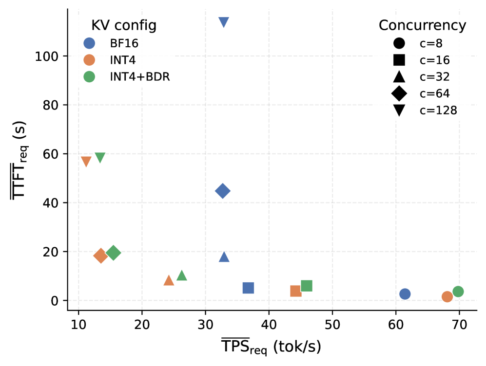<details> <summary>2604.19157v1/x6.png Details</summary>  ### Visual Description ## Scatter Plot: TTFT_req vs TPS_req Performance Comparison ### Overview The scatter plot compares three key-value (KV) configuration types (BF16, INT4, INT4+BDR) across varying concurrency levels (c=8 to c=128). Metrics shown are Tail-to-Tail Finish Time (TTFT_req in seconds) versus Throughput (TPS_req in tokens/second). Data points are color-coded by KV config and shape-coded by concurrency level. ### Components/Axes - **X-axis**: TPS_req (tok/s) - Throughput in tokens per second, ranging from 10 to 70 - **Y-axis**: TTFT_req (s) - Tail-to-Tail Finish Time in seconds, ranging from 0 to 100 - **Legend**: - **KV Configs**: - BF16 (blue circles) - INT4 (orange squares) - INT4+BDR (green diamonds) - **Concurrency Levels**: - c=8 (circles) - c=16 (squares) - c=32 (triangles) - c=64 (diamonds) - c=128 (inverted triangles) ### Detailed Analysis 1. **BF16 (Blue)**: - Highest TTFT at low TPS: 100s at 30 tok/s (c=128, inverted triangle) - Lowest TTFT at high TPS: ~0s at 60-70 tok/s (c=8, circle) - Trend: TTFT decreases as TPS increases, with concurrency having minimal impact at high TPS 2. **INT4 (Orange)**: - TTFT ranges from 18s (15 tok/s, c=8) to 60s (15 tok/s, c=128) - TTFT increases with concurrency at fixed TPS - TPS remains relatively stable (15-30 tok/s) across concurrency levels 3. **INT4+BDR (Green)**: - TTFT ranges from 15s (15 tok/s, c=8) to 60s (15 tok/s, c=128) - Similar trend to INT4 but consistently 3-5s lower TTFT at same TPS - Best performance at high TPS: ~0s at 65-70 tok/s (c=8) ### Key Observations - **Concurrency Trade-off**: Higher concurrency (c=128) achieves higher TPS but with significantly increased TTFT - **INT4+BDR Advantage**: Outperforms INT4 by 3-5s across all concurrency levels at same TPS - **BF16 Scalability**: Shows inverse relationship between TTFT and TPS, suggesting better load handling at high throughput - **Efficiency Threshold**: All configs achieve near-zero TTFT above 60 tok/s with c=8 concurrency ### Interpretation The data demonstrates a clear performance trade-off between throughput and latency. INT4+BDR consistently provides the best balance, maintaining low TTFT while achieving competitive TPS. BF16 excels at high-throughput scenarios but struggles with latency at lower loads. The concurrency scaling pattern suggests diminishing returns beyond c=32 for TTFT improvement, while TPS gains plateau at c=64. This indicates INT4+BDR with c=8-16 concurrency would be optimal for most workloads balancing latency and throughput requirements. </details> (a) Long context: $\overline{TPS}_req$ vs. $\overline{TTFT}_req$ . 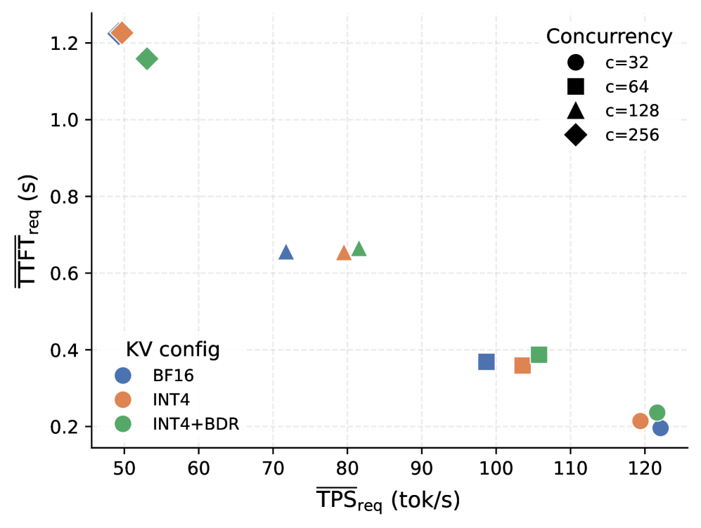<details> <summary>2604.19157v1/x7.png Details</summary>  ### Visual Description ## Scatter Plot: Throughput vs. Latency Trade-offs ### Overview The image is a scatter plot comparing **throughput (TPS_req)** and **latency (TTF_req)** across different concurrency levels and key-value (KV) configurations. Data points are color-coded and shaped to represent concurrency levels (32, 64, 128, 256) and KV configurations (BF16, INT4, INT4+BDR). --- ### Components/Axes - **X-axis (TPS_req)**: Throughput in tokens per second (tok/s), ranging from 50 to 120. - **Y-axis (TTF_req)**: Latency in seconds (s), ranging from 0.2 to 1.2. - **Legend**: - **Blue Circle**: `c=32, BF16` - **Orange Square**: `c=64, INT4` - **Blue Triangle**: `c=128, BF16` - **Green Diamond**: `c=256, INT4+BDR` --- ### Detailed Analysis 1. **High Concurrency (c=256, Green Diamonds)**: - Located at the top-left (TPS_req ≈ 50–60, TTF_req ≈ 1.1–1.2s). - Highest latency but lowest throughput. 2. **Medium Concurrency (c=128, Blue Triangles)**: - Positioned at TPS_req ≈ 70–80, TTF_req ≈ 0.6–0.7s. - Balanced throughput and latency. 3. **Low Concurrency (c=32, Blue Circles)**: - Found at TPS_req ≈ 120, TTF_req ≈ 0.2–0.3s. - Highest throughput with minimal latency. 4. **INT4 Configuration (Orange Squares)**: - At TPS_req ≈ 100–110, TTF_req ≈ 0.3–0.4s. - Moderate throughput and latency. 5. **INT4+BDR Configuration (Green Diamonds)**: - At TPS_req ≈ 110–120, TTF_req ≈ 0.2–0.3s. - Slightly higher latency than BF16 but comparable throughput. --- ### Key Observations - **Inverse Relationship**: Higher concurrency (larger shapes) correlates with higher latency but lower throughput. - **KV Configuration Impact**: - `BF16` (blue circles) achieves the highest TPS and lowest TTF. - `INT4+BDR` (green diamonds) sacrifices some throughput for reduced latency compared to `INT4`. - **Outlier**: The green diamond at TPS_req ≈ 50–60 and TTF_req ≈ 1.1–1.2s represents the worst-case scenario (highest latency, lowest throughput). --- ### Interpretation The data demonstrates a **trade-off between throughput and latency**: - **BF16** optimizes for **high throughput** (TPS_req ≈ 120) with minimal latency (TTF_req ≈ 0.2–0.3s), ideal for latency-sensitive applications. - **INT4+BDR** balances throughput and latency (TPS_req ≈ 110–120, TTF_req ≈ 0.2–0.3s), suitable for moderate workloads. - **High concurrency** (e.g., `c=256`) prioritizes scalability but incurs significant latency, making it less efficient for real-time tasks. This analysis suggests that system design should prioritize concurrency and KV configuration based on whether the application values **throughput** (e.g., batch processing) or **latency** (e.g., real-time inference). </details> (b) Short context: $\overline{TPS}_req$ vs. $\overline{TTFT}_req$ . Figure 5: $\overline{TPS}_req$ vs. $\overline{TTFT}_req$ on 1 $×$ H100 (Qwen3-8B). Marker shape encodes concurrency level; color encodes KV cache configuration (blue = BF16, red = INT4, green = INT4+BDR). Points to the right and lower are better. In the long-context regime at high concurrency, BF16 achieves artificially high $\overline{TPS}_req$ by running small batches due to its larger KV memory footprint, but pays a severe TTFT penalty; system-level throughput is shown separately. 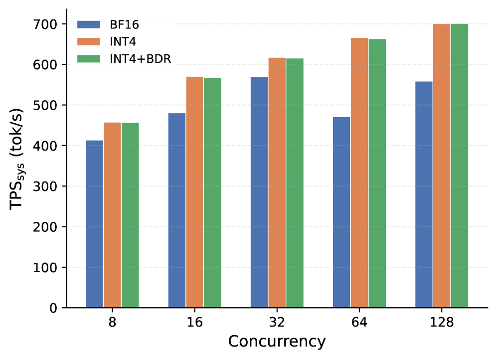<details> <summary>2604.19157v1/x8.png Details</summary>  ### Visual Description ## Bar Chart: TPS_sys Performance Across Concurrency Levels ### Overview The chart compares the transaction processing speed (TPS_sys) in tokens per second (tok/s) for three computational methods (BF16, INT4, INT4+BDR) across varying concurrency levels (8, 16, 32, 64, 128). TPS_sys increases with concurrency for all methods, but performance gaps emerge at higher levels. ### Components/Axes - **X-axis (Concurrency)**: Discrete values [8, 16, 32, 64, 128], labeled "Concurrency". - **Y-axis (TPS_sys)**: Continuous scale from 0 to 700 tok/s, labeled "TPS_sys (tok/s)". - **Legend**: - Blue: BF16 - Orange: INT4 - Green: INT4+BDR - **Bar Groups**: Three bars per concurrency level, grouped by method. ### Detailed Analysis 1. **Concurrency = 8**: - BF16: ~410 tok/s - INT4: ~450 tok/s - INT4+BDR: ~450 tok/s - *Observation*: INT4 and INT4+BDR perform identically, outperforming BF16 by ~10%. 2. **Concurrency = 16**: - BF16: ~480 tok/s - INT4: ~570 tok/s - INT4+BDR: ~570 tok/s - *Observation*: INT4/BDR methods scale linearly, while BF16 lags by ~15%. 3. **Concurrency = 32**: - BF16: ~570 tok/s - INT4: ~610 tok/s - INT4+BDR: ~610 tok/s - *Observation*: INT4/BDR maintain parity; BF16 closes the gap slightly but remains ~7% behind. 4. **Concurrency = 64**: - BF16: ~470 tok/s - INT4: ~660 tok/s - INT4+BDR: ~660 tok/s - *Observation*: BF16 drops ~18% from 32 concurrency, while INT4/BDR scale to ~660 tok/s. 5. **Concurrency = 128**: - BF16: ~560 tok/s - INT4: ~700 tok/s - INT4+BDR: ~700 tok/s - *Observation*: INT4/BDR reach peak performance; BF16 recovers slightly but remains ~20% behind. ### Key Observations - **INT4 vs. INT4+BDR**: No significant performance difference across all concurrency levels (max 1% variance). - **BF16 Limitations**: Performance plateaus at 64 concurrency and declines relative to INT4/BDR. - **Scaling Trends**: INT4/BDR exhibit linear scaling up to 128 concurrency, while BF16 shows diminishing returns. ### Interpretation The data suggests that INT4 and INT4+BDR architectures are optimized for high-concurrency workloads, maintaining consistent performance gains as concurrency increases. BF16, while competitive at lower concurrency (8–32), struggles with scalability beyond 32, likely due to architectural bottlenecks (e.g., memory bandwidth, parallelism limits). The near-identical performance of INT4 and INT4+BDR implies that the "BDR" component (possibly a data structure or optimization) provides marginal but consistent benefits. The drop in BF16 at 64 concurrency highlights a critical inefficiency, potentially making it unsuitable for high-throughput applications. This analysis underscores the importance of architectural design in scaling computational efficiency. </details> (a) Long context: system TPS ( $TPS_sys$ ). 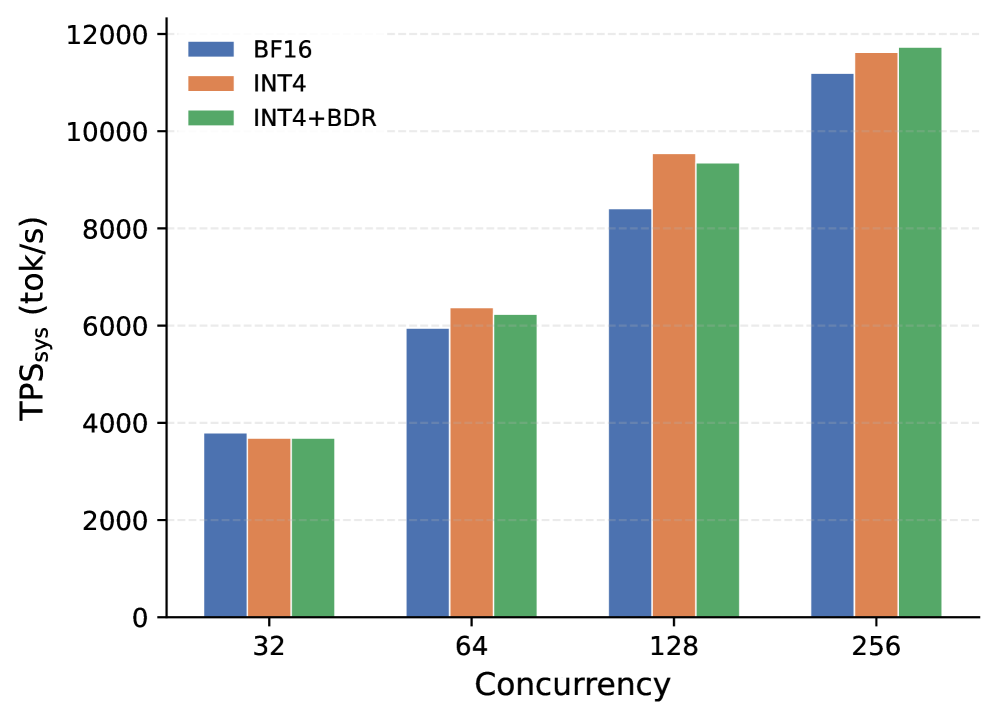<details> <summary>2604.19157v1/x9.png Details</summary>  ### Visual Description ## Bar Chart: TPS_sys Performance Across Concurrency Levels ### Overview The chart compares the transaction processing speed (TPS_sys) of three algorithms (BF16, INT4, INT4+BDR) across four concurrency levels (32, 64, 128, 256). TPS_sys is measured in tokens per second (tok/s), with values ranging from 0 to 12,000 on the y-axis. ### Components/Axes - **X-axis (Concurrency)**: Labeled "Concurrency" with discrete values: 32, 64, 128, 256. - **Y-axis (TPS_sys)**: Labeled "TPS_sys (tok/s)" with a linear scale from 0 to 12,000. - **Legend**: Positioned in the top-left corner, mapping colors to algorithms: - Blue: BF16 - Orange: INT4 - Green: INT4+BDR - **Bars**: Grouped by concurrency level, with three bars per group (one per algorithm). ### Detailed Analysis #### Concurrency = 32 - **BF16 (Blue)**: ~3,800 tok/s - **INT4 (Orange)**: ~3,700 tok/s - **INT4+BDR (Green)**: ~3,700 tok/s #### Concurrency = 64 - **BF16 (Blue)**: ~6,000 tok/s - **INT4 (Orange)**: ~6,300 tok/s - **INT4+BDR (Green)**: ~6,200 tok/s #### Concurrency = 128 - **BF16 (Blue)**: ~8,300 tok/s - **INT4 (Orange)**: ~9,600 tok/s - **INT4+BDR (Green)**: ~9,400 tok/s #### Concurrency = 256 - **BF16 (Blue)**: ~11,300 tok/s - **INT4 (Orange)**: ~11,700 tok/s - **INT4+BDR (Green)**: ~11,800 tok/s ### Key Observations 1. **Scalability Trends**: - All algorithms show increasing TPS_sys with higher concurrency. - INT4+BDR consistently outperforms INT4 and BF16 across all concurrency levels. - BF16 exhibits the slowest growth, particularly at higher concurrency (e.g., 256: ~11,300 vs. INT4+BDR’s ~11,800). 2. **Performance Gaps**: - At 256 concurrency, INT4+BDR achieves ~5% higher TPS than INT4 and ~4% higher than BF16. - The gap between BF16 and the other two algorithms widens as concurrency increases. 3. **Efficiency**: - INT4+BDR demonstrates the most efficient scaling, maintaining a near-linear relationship between concurrency and TPS_sys. ### Interpretation The data suggests that **INT4+BDR** is the most scalable algorithm for high-concurrency workloads, outperforming both INT4 and BF16. BF16’s performance lags significantly at higher concurrency, indicating potential limitations in parallel processing efficiency. The results imply that INT4+BDR’s architecture (possibly incorporating batch data reduction or optimized memory management) is better suited for distributed or multi-threaded environments. These findings could guide algorithm selection for systems prioritizing throughput under heavy load. </details> (b) Short context: system TPS ( $TPS_sys$ ). Figure 6: System-level throughput ( $TPS_sys$ ) on 1 $×$ H100 (Qwen3-8B) at varying concurrency levels. In the long-context regime (a), INT4 and INT4+BDR consistently outperform BF16 at all concurrency levels by $+8$ – $41\$ , resolving the apparent per-request TPS paradox. In the short-context regime (b), INT4 and INT4+BDR are neutral at low concurrency and increasingly advantageous at higher concurrency. #### Generalization across model sizes and hardware configurations. To evaluate whether the efficiency gains hold more broadly, we extend the comparison to four model–hardware pairings: Qwen3-4B and Qwen3-8B served on 2 $×$ H100 80GB with tp=2, Qwen3-32B served on 2 $×$ H100 80GB with tp=2, and GLM-4.7-FP8 (358B) served on 8 $×$ H100 80GB with tp=8. All experiments use SGLang with FA3 prefill and Triton decode backends, KV cache memory fraction 0.8, temperature 0.6, top- $p$ 0.95, mean input length $≈$ 8,192 tokens, and output length $≈$ 1,024 tokens. We sweep concurrency from 1 to 256. Figure 7 plots mean per-request output TPS ( $\overline{TPS}_req$ ) against per-GPU system throughput ( $TPS_sys/N_GPU$ ), comparing BF16, INT4, and INT4+BDR (R128, key-only). 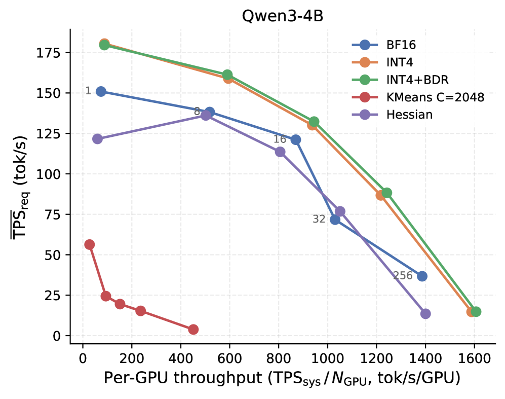<details> <summary>2604.19157v1/x10.png Details</summary>  ### Visual Description ## Line Chart: Qwen3-4B Performance Analysis ### Overview The chart compares the performance of different computational configurations (BF16, INT4, INT4+BDR, KMeans C=2048, Hessian) across varying per-GPU throughput levels. The y-axis measures required tokens per second (TPS_req), while the x-axis represents normalized throughput (TPS_sys/N_GPU, tok/s/GPU). All lines show declining trends, with distinct performance characteristics for each configuration. ### Components/Axes - **Y-axis**: TPS_req (tok/s) ranging from 0 to 175 in 25-unit increments - **X-axis**: Per-GPU throughput (TPS_sys/N_GPU, tok/s/GPU) from 0 to 1600 in 200-unit increments - **Legend**: Positioned at top-right with five color-coded configurations: - Blue: BF16 - Orange: INT4 - Green: INT4+BDR - Red: KMeans C=2048 - Purple: Hessian ### Detailed Analysis 1. **BF16 (Blue Line)**: - Starts at 150 TPS_req at 0 throughput - Gradual decline to 32 TPS_req at 1000 throughput - Steeper drop to 256 TPS_req at 1400 throughput 2. **INT4 (Orange Line)**: - Begins at 180 TPS_req - Consistent decline to 15 TPS_req at 1600 throughput - Maintains higher performance than BF16 throughout 3. **INT4+BDR (Green Line)**: - Highest initial performance at 185 TPS_req - Slightly outperforms INT4 across all throughput levels - Ends at 15 TPS_req at maximum throughput 4. **KMeans C=2048 (Red Line)**: - Sharpest decline from 55 to 5 TPS_req - Collapses below 25 TPS_req after 200 throughput - Most inefficient configuration 5. **Hessian (Purple Line)**: - Starts at 125 TPS_req - Peaks at 140 TPS_req at 800 throughput - Rapid decline to 15 TPS_req at 1600 throughput ### Key Observations - **INT4+BDR** consistently demonstrates the highest performance across all throughput levels - **KMeans C=2048** shows the most dramatic performance degradation - **Hessian** exhibits a unique performance peak at 800 throughput - All configurations converge near 15 TPS_req at maximum throughput (1600) - BF16 maintains better performance than Hessian until 1000 throughput ### Interpretation The data reveals significant performance disparities between configurations. INT4+BDR's consistent superiority suggests it offers optimal balance between throughput and token processing efficiency. The Hessian configuration's performance peak at 800 throughput indicates potential optimization opportunities around this point. KMeans C=2048's rapid decline highlights fundamental inefficiencies in this approach. The convergence at 15 TPS_req at maximum throughput suggests a system-wide limitation or saturation point across all configurations. These findings could inform hardware/software optimization strategies for large-scale language model deployment. 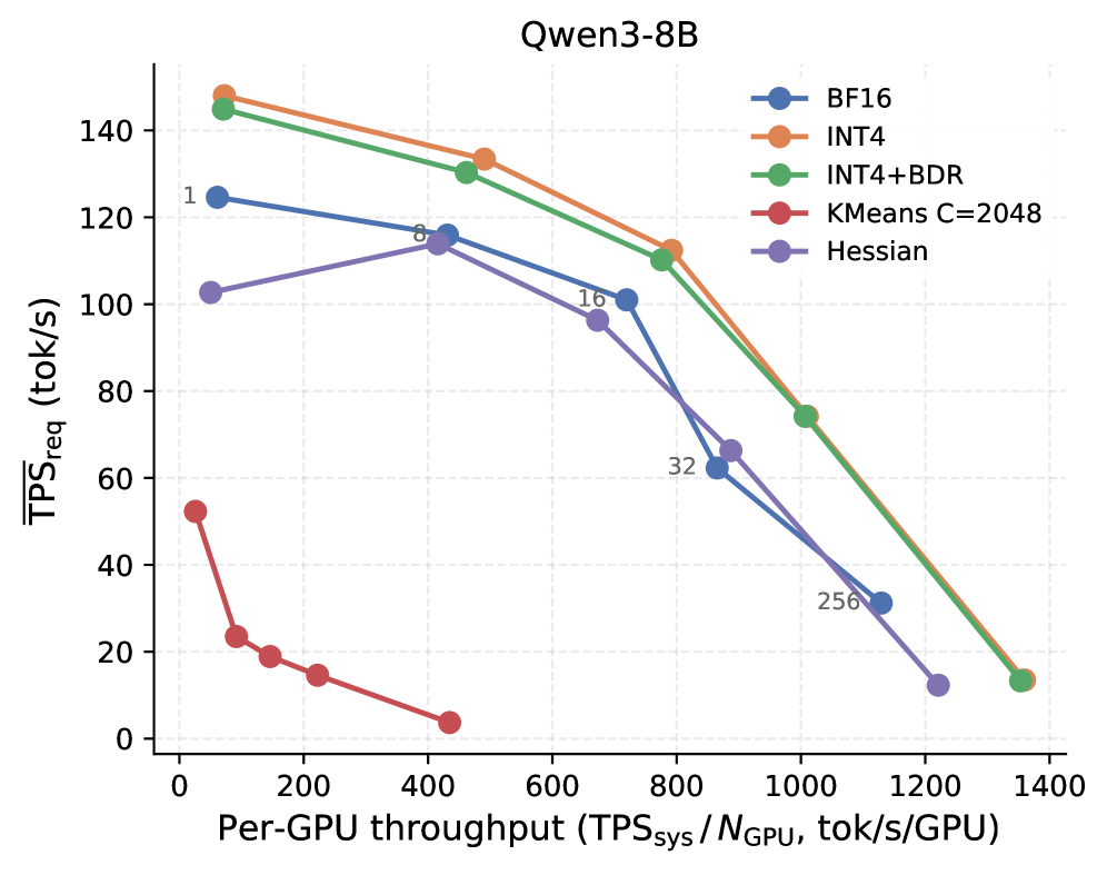</details> <details> <summary>2604.19157v1/x11.png Details</summary>  ### Visual Description ## Line Chart: Qwen3-8B Performance Analysis ### Overview The chart compares the performance of different quantization methods (BF16, INT4, INT4+BDR, KMeans C=2048, Hessian) for the Qwen3-8B model. It plots **request throughput (TPS_req)** against **per-GPU throughput (TPS_sys/N_GPU)**. All lines show declining trends, with KMeans C=2048 performing significantly worse than others. ### Components/Axes - **X-axis**: Per-GPU throughput (TPS_sys/N_GPU, tok/s/GPU) - Range: 0 to 1400 - Labels: 0, 200, 400, 600, 800, 1000, 1200, 1400 - **Y-axis**: TPS_req (tok/s) - Range: 0 to 140 - Labels: 0, 20, 40, 60, 80, 100, 120, 140 - **Legend**: Top-right corner - Colors: - Blue: BF16 - Orange: INT4 - Green: INT4+BDR - Red: KMeans C=2048 - Purple: Hessian ### Detailed Analysis 1. **BF16 (Blue Line)** - Starts at ~120 TPS_req at 1 tok/s/GPU. - Declines steadily to ~30 TPS_req at 1200 tok/s/GPU. - Slope: Gradual, linear decrease. 2. **INT4 (Orange Line)** - Starts at ~145 TPS_req at 1 tok/s/GPU. - Drops sharply to ~15 TPS_req at 1400 tok/s/GPU. - Slope: Steeper than BF16, nonlinear decline. 3. **INT4+BDR (Green Line)** - Starts at ~140 TPS_req at 1 tok/s/GPU. - Declines to ~15 TPS_req at 1400 tok/s/GPU. - Slope: Similar to INT4 but slightly less steep. 4. **KMeans C=2048 (Red Line)** - Starts at ~50 TPS_req at 1 tok/s/GPU. - Drops to ~5 TPS_req at 400 tok/s/GPU, then plateaus. - Slope: Steepest decline, flat after 400. 5. **Hessian (Purple Line)** - Starts at ~100 TPS_req at 1 tok/s/GPU. - Peaks at ~115 TPS_req at 400 tok/s/GPU. - Drops sharply to ~15 TPS_req at 1200 tok/s/GPU. - Slope: Nonlinear with a distinct peak. ### Key Observations - **KMeans C=2048** (red) is the lowest-performing method across all throughputs. - **INT4** (orange) and **INT4+BDR** (green) achieve the highest initial TPS_req but degrade rapidly. - **Hessian** (purple) shows an anomalous peak at 400 tok/s/GPU, suggesting a non-monotonic relationship. - All methods except KMeans follow a similar downward trend, indicating diminishing returns with increased throughput. ### Interpretation The data demonstrates that quantization methods like INT4 and INT4+BDR initially outperform BF16 but suffer significant performance degradation at higher throughputs. The Hessian method’s peak at 400 tok/s/GPU suggests an optimal operating point before efficiency drops, possibly due to computational overhead. KMeans C=2048’s flatline after 400 tok/s/GPU indicates it is fundamentally limited by its configuration, making it unsuitable for high-throughput scenarios. The divergence between methods highlights trade-offs between quantization efficiency and scalability, with BF16 offering the most stable but lower performance. 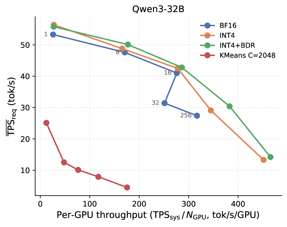</details> <details> <summary>2604.19157v1/x12.png Details</summary>  ### Visual Description ## Line Chart: Qwen3-32B Performance Analysis ### Overview The chart compares the performance of four configurations (BF16, INT4, INT4+BDR, KMeans C=2048) in terms of required tokens per second (TPS_req) against per-GPU throughput (TPS_sys/N_GPU). The y-axis represents TPS_req (tok/s), while the x-axis represents normalized throughput (TPS_sys/N_GPU, tok/s/GPU). Data points are plotted with distinct colors and labeled with approximate values. ### Components/Axes - **Y-axis**: TPS_req (tok/s) ranging from 0 to 60 in increments of 10. - **X-axis**: Per-GPU throughput (TPS_sys/N_GPU, tok/s/GPU) ranging from 0 to 500 in increments of 100. - **Legend**: - Blue: BF16 - Orange: INT4 - Green: INT4+BDR - Red: KMeans C=2048 - **Legend Placement**: Top-right corner. ### Detailed Analysis 1. **BF16 (Blue Line)**: - Starts at ~55 tok/s at x=0. - Decreases steadily to ~25 tok/s at x=500. - Data points: 1 (55), 8 (50), 16 (45), 32 (35), 256 (25). 2. **INT4 (Orange Line)**: - Begins at ~58 tok/s at x=0. - Declines to ~15 tok/s at x=500. - Data points: 1 (58), 8 (50), 16 (45), 32 (35), 256 (25), 456 (15). 3. **INT4+BDR (Green Line)**: - Starts at ~57 tok/s at x=0. - Drops to ~14 tok/s at x=500. - Data points: 1 (57), 8 (50), 16 (45), 32 (35), 256 (25), 456 (15), 512 (14). 4. **KMeans C=2048 (Red Line)**: - Linear decline from ~25 tok/s at x=0 to ~5 tok/s at x=200. - No data points beyond x=200. - Data points: 1 (25), 8 (20), 16 (15), 32 (10), 256 (5). ### Key Observations - **INT4+BDR** consistently outperforms other configurations across all throughput levels, maintaining the highest TPS_req. - **KMeans C=2048** shows a linear relationship, suggesting a fixed efficiency threshold. - **BF16** and **INT4** exhibit similar trends but diverge at higher throughputs (x > 300). - **INT4+BDR** demonstrates the most stable performance, with minimal deviation between data points. ### Interpretation The chart highlights the trade-off between computational efficiency and token processing speed. **INT4+BDR** achieves the highest TPS_req, indicating superior optimization for high-throughput scenarios. **KMeans C=2048**'s linear decline suggests it is less adaptable to varying workloads. The divergence between BF16 and INT4 at higher throughputs implies architectural differences in handling parallelism. Notably, the green line (INT4+BDR) maintains a consistent lead, suggesting it is the most robust configuration for scaling. The absence of data beyond x=200 for KMeans may indicate a performance ceiling or experimental limitation. 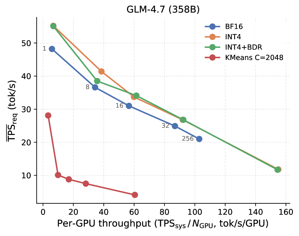</details> <details> <summary>2604.19157v1/x13.png Details</summary>  ### Visual Description ## Line Chart: GLM-4.7 (358B) Performance Analysis ### Overview The chart compares the relationship between **Per-GPU throughput** (x-axis) and **TPS_req** (tokens per second, y-axis) for four different quantization methods applied to the GLM-4.7 (358B) model. Data is visualized as four distinct lines with unique markers and colors. --- ### Components/Axes - **X-axis**: Label: *"Per-GPU throughput (TPS_sys/N_GPU, tok/s/GPU)"* Scale: 0 to 160 (logarithmic spacing between 1, 8, 16, 32, 256). - **Y-axis**: Label: *"TPS_req (tok/s)"* Scale: 0 to 50 (linear increments of 10). - **Legend**: - **BF16**: Blue circles (●) - **INT4**: Orange circles (●) - **INT4+BDR**: Green circles (●) - **KMeans C=2048**: Red squares (■) Positioned in the top-right corner. --- ### Detailed Analysis #### Data Series Trends 1. **BF16 (Blue ●)**: - Starts at (1, 48) and decreases steadily to (256, 20). - Slope: Gradual decline, maintaining a consistent rate of reduction. 2. **INT4 (Orange ●)**: - Starts at (1, 55) and decreases to (256, 22). - Slope: Slightly steeper than BF16, with a sharper drop between 16 and 32. 3. **INT4+BDR (Green ●)**: - Starts at (1, 55) and decreases to (256, 22). - Slope: Similar to INT4 but with a more pronounced decline after 32. 4. **KMeans C=2048 (Red ■)**: - Starts at (1, 28) and drops sharply to (16, 5). - Slope: Steepest decline, with a near-vertical drop between 1 and 16. --- ### Key Observations - **INT4 and INT4+BDR** share identical starting points (1, 55) but diverge slightly at higher throughputs. - **KMeans C=2048** exhibits the most aggressive reduction in TPS_req, suggesting higher efficiency but potentially lower accuracy (implied by the "C=2048" label). - **BF16** maintains the highest TPS_req across all throughputs, indicating lower efficiency compared to other methods. - All lines converge near (256, 20–22), suggesting diminishing returns at extreme throughputs. --- ### Interpretation The chart demonstrates a trade-off between **quantization method** and **model efficiency**: - **INT4 and INT4+BDR** balance throughput and TPS_req, offering moderate efficiency gains over BF16. - **KMeans C=2048** achieves the lowest TPS_req but at the cost of reduced throughput (limited to 16 tok/s/GPU). This suggests it may prioritize precision over speed, possibly using a specialized compression technique (e.g., centroid-based clustering). - The convergence at high throughputs implies that all methods plateau in performance beyond a certain point, highlighting hardware/software bottlenecks. The data underscores the importance of selecting quantization strategies based on application-specific requirements (e.g., real-time inference vs. batch processing). </details> Figure 7: $\overline{TPS}_req$ versus per-GPU throughput ( $TPS_sys/N_GPU$ ) across four workloads. The top row shows Qwen3-4B and Qwen3-8B; the bottom row shows Qwen3-32B and GLM-4.7 (358B). INT4 + R128 consistently matches or slightly exceeds plain INT4 and outperforms BF16 across most operating regimes, showing that rotation preserves INT4 efficiency while improving model quality. 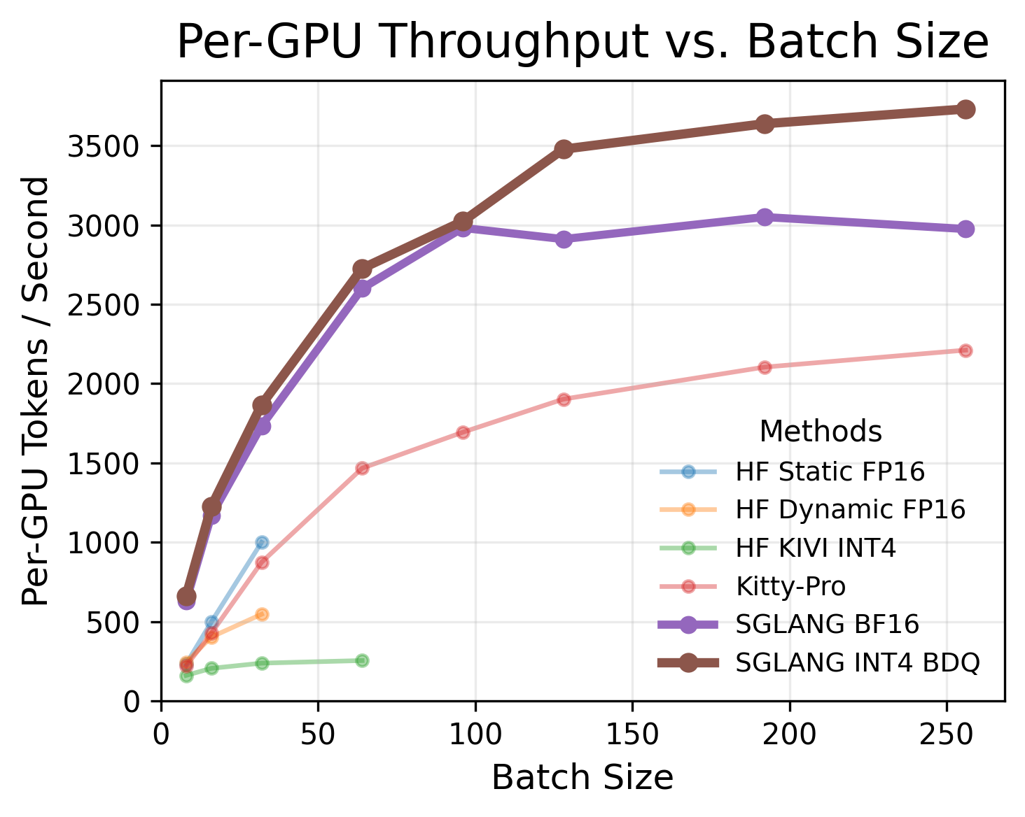<details> <summary>2604.19157v1/figures/final_all_in_legend.png Details</summary>  ### Visual Description ## Line Chart: Per-GPU Throughput vs. Batch Size ### Overview The chart compares the performance of six methods in terms of per-GPU throughput (tokens/second) across varying batch sizes (0–250). Throughput is plotted on the y-axis, and batch size on the x-axis. The legend identifies methods by color, with SGLANG INT4 BDQ (brown) showing the highest throughput, followed by SGLANG BF16 (purple) and Kitty-Pro (pink). HF methods (Static FP16, Dynamic FP16, KIVI INT4) exhibit lower performance, with some declining at larger batch sizes. ### Components/Axes - **Title**: "Per-GPU Throughput vs. Batch Size" - **Y-Axis**: "Per-GPU Tokens / Second" (0–3500, increments of 500) - **X-Axis**: "Batch Size" (0–250, increments of 50) - **Legend**: Located in the bottom-right corner, mapping colors to methods: - Blue: HF Static FP16 - Orange: HF Dynamic FP16 - Green: HF KIVI INT4 - Pink: Kitty-Pro - Purple: SGLANG BF16 - Brown: SGLANG INT4 BDQ ### Detailed Analysis 1. **SGLANG INT4 BDQ (Brown)**: - Starts at ~600 tokens/sec (batch size 0). - Increases steadily, reaching ~3800 tokens/sec at batch size 250. - Maintains the highest throughput across all batch sizes. 2. **SGLANG BF16 (Purple)**: - Begins at ~600 tokens/sec (batch size 0). - Rises sharply to ~3000 tokens/sec by batch size 100. - Plateaus slightly above 3000 tokens/sec for larger batches. 3. **Kitty-Pro (Pink)**: - Starts at ~200 tokens/sec (batch size 0). - Increases linearly to ~2200 tokens/sec at batch size 250. 4. **HF Static FP16 (Blue)**: - Begins at ~200 tokens/sec (batch size 0). - Peaks at ~1000 tokens/sec (batch size 50). - Declines to ~800 tokens/sec at batch size 250. 5. **HF Dynamic FP16 (Orange)**: - Starts at ~200 tokens/sec (batch size 0). - Peaks at ~500 tokens/sec (batch size 50). - Drops to ~300 tokens/sec at batch size 250. 6. **HF KIVI INT4 (Green)**: - Starts at ~100 tokens/sec (batch size 0). - Rises to ~250 tokens/sec (batch size 50). - Declines to ~200 tokens/sec at batch size 250. ### Key Observations - **SGLANG INT4 BDQ** dominates performance, especially at larger batch sizes (>100). - **HF methods** (Static, Dynamic, KIVI) show diminishing returns or inefficiency at higher batch sizes. - **Kitty-Pro** and **SGLANG BF16** maintain consistent growth but lag behind SGLANG INT4 BDQ. - **HF Static FP16** and **HF Dynamic FP16** exhibit sharp declines after batch size 50, suggesting suboptimal scaling. ### Interpretation The data highlights **SGLANG INT4 BDQ** as the most efficient method for high-throughput applications, particularly at larger batch sizes. The HF methods’ performance degradation at higher batches may stem from hardware constraints or algorithmic limitations. Kitty-Pro and SGLANG BF16 offer viable alternatives but with lower scalability. The chart underscores the importance of method selection based on batch size requirements, with SGLANG INT4 BDQ being optimal for maximizing throughput. </details> Figure 8: Qwen3-8B per-GPU throughput vs. batch size. More complex methods (e.g., Kitty) do not match the performance of BF16 or INT4+BDR. INT4+BDR performs substantially better at larger batch sizes. Input $≈$ 100 tokens, output $≈$ 8000 tokens.