# The Spectral Lifecycle of Transformer Training: Transient Compression Waves, Persistent Spectral Gradients, and the Q/K–V Asymmetry
**Authors**: Yi Liu
## Abstract
We present the first systematic study of weight matrix singular value spectra during transformer pretraining, tracking full SVD decompositions of every weight matrix at 25-step intervals across three model scales (30M–285M parameters). We discover three phenomena: (1) Transient Compression Waves: stable rank compression propagates as a traveling wave from early to late layers, creating a dramatic gradient that peaks early then reverses —late layers eventually over-compress past early layers. (2) Persistent Spectral Gradients: the power-law exponent $α$ develops a permanent depth gradient forming a non-monotonic inverted-U in deeper models, with peaks shifting toward earlier layers as depth increases. (3) Q/K–V Functional Asymmetry: value/output projections compress uniformly while query/key projections carry the full depth-dependent dynamics. The dissociation between transient compression and persistent spectral shape reveals that rank and spectral shape encode fundamentally different information about training. We formalize this as a two-timescale dynamical model and derive scaling laws ( $Δα∝ L^0.26$ , $R^2{=}0.99$ ). We validate on nine models across three families (custom, GPT-2, Pythia; 30M–1B parameters; 8–36 layers), demonstrate that $α$ predicts layer importance ( $ρ{=}0.69$ – $0.84$ , $p{<}0.02$ ), and show that spectral-guided pruning outperforms Last-N heuristics by $1.1{×}$ – $3.6{×}$ across seven models in two families (GPT-2 124M–774M, Pythia 160M–1B), with worst-vs-best gaps up to $23.7{×}$ confirming the causal role of spectral structure.
## 1 Introduction
Training large language models costs millions of dollars, yet we understand surprisingly little about what happens inside them during training. Despite advances in scaling laws (Kaplan et al., 2020; Hoffmann et al., 2022), architectures (Gu and Dao, 2024), and training recipes (Touvron et al., 2023), practitioners monitor loss curves—a single scalar—hoping that billions of parameters evolve sensibly.
Random matrix theory (RMT) offers a richer lens. The Heavy-Tail Self-Regularization (HT-SR) framework (Martin and Mahoney, 2021; Martin et al., 2021) showed that trained networks exhibit heavy-tailed singular value distributions correlating with generalization, and recent work has exploited this for pruning (Lu et al., 2024) and studied per-matrix spectral dynamics (Yunis et al., 2024). However, the critical question of how spectral structure varies across layers and evolves over training —the spatiotemporal picture—remains unexplored. Existing work either examines static snapshots or tracks individual matrices without studying inter-layer relationships.
We conduct the first comprehensive spectral time-lapse of transformer pretraining, tracking full SVDs of every weight matrix at fine-grained intervals across multiple scales. This yields a spatiotemporal dataset of over 150,000 SVD snapshots that reveals phenomena invisible to scalar monitoring.
Our central discovery is a dissociation between compression and spectral shape: the compression (stable rank reduction) follows a transient wave that eventually equilibrates, while the spectral shape (power-law exponent $α$ ) develops a permanent gradient. Compression measures how much structure has emerged; $α$ measures what kind.
#### Contributions.
(1) We discover transient compression waves propagating from early to late layers at ${∼}$ 80–100 steps/layer, with a gradient that reverses from negative to positive as late layers over-compress (Section 4.1). (2) We identify persistent spectral gradients where $α$ forms a non-monotonic inverted-U that strengthens throughout training, with the peak shifting toward earlier relative depth in deeper models (Section 4.2). (3) We reveal Q/K–V functional asymmetry: V/O projections compress uniformly while Q/K carry depth-dependent dynamics (Section 4.3). (4) We formalize a two-timescale dynamical model with scaling laws (Section 5). (5) We validate on pretrained GPT-2 (124M–774M) and Pythia (160M–1B) models with training checkpoints confirming the theory (Section 6). (6) We show $α$ predicts layer importance and enables spectral-guided pruning that outperforms Last-N by $1.1$ – $3.6×$ across seven models in two families: GPT-2 (124M–774M) and Pythia (160M–1B), holding from 12 to 36 layers (Section 7).
## 2 Related Work
#### RMT and Spectral Analysis.
The HT-SR framework (Martin and Mahoney, 2021; Martin et al., 2021) established that trained networks exhibit heavy-tailed spectra correlating with generalization. Lu et al. (2024) leveraged $α$ for layerwise pruning ratios in pretrained LLMs, showing per-layer $α$ variation predicts prunability. We complement this by revealing how $α$ gradients emerge during training and showing they predict layer importance, not just prunability. Staats et al. (2024) showed small singular values carry meaning. Huang et al. (2025) used spectral density evolution for early stopping. All analyze static or coarse-grained snapshots; we track fine-grained dynamics.
#### Spectral Dynamics of Weights.
Most closely related, Yunis et al. (2024) study singular value and vector dynamics during optimization, identifying a “bulk-plus-spike” pattern where a few top singular values grow while the bulk remains near initialization. Our work differs in three ways: (i) we analyze inter-layer gradients and their temporal evolution, not individual-matrix dynamics; (ii) we discover the transient/persistent dissociation between compression and spectral shape—a phenomenon invisible when studying single matrices; (iii) we validate across 9 models in 3 families including training checkpoints. Xu (2026) study spectral edge dynamics of parameter updates; Olsen et al. (2025) develop an SDE framework for singular value evolution; Liu et al. (2025) study activation spectra. Our analysis of weight spectra across depth reveals complementary spatiotemporal phenomena.
#### Training Dynamics.
Grokking (Power et al., 2022; Truong et al., 2026), the break-even point (Jastrzebski et al., 2020), edge of stability (Cohen et al., 2021), and double descent (Nakkiran et al., 2021) reveal phase transitions. Our spectral perspective uncovers a novel transient/persistent dissociation invisible to scalar metrics.
#### Per-Layer Analysis.
Layer roles have been studied through probing (Tenney et al., 2019), knowledge storage (Geva et al., 2022), induction heads (Olsson et al., 2022), and layer pruning (Men et al., 2024). Our spectral metrics capture layer specialization from weights alone, without input data.
## 3 Method
### 3.1 Spectral Metrics
For each weight matrix $W∈ℝ^m× n$ with singular values $σ_1≥⋯≥σ_k$ ( $k=\min(m,n)$ ), we track:
Stable Rank: $R_s(W)=\|W\|_F^2/\|W\|_2^2=∑_iσ_i^2/σ_1^2$ , measuring effective dimensionality.
Weighted Alpha: $\logσ_i≈-α\log i+c$ for $i=1,…,\lfloor 0.2k\rfloor$ , measuring power-law tail heaviness.
Spectral Entropy: $H=-(\log_2k)^-1∑_ip_i\log_2p_i$ , $p_i=σ_i^2/\|\boldsymbol{σ}\|_2^2$ , an independent confirmation metric.
The compression onset for layer $l$ is the first step where $R_s$ drops below $0.9R_s^(l)(0)$ . Fitting $t_onset^(l)≈ v· l+t_0$ yields the compression wave velocity $v$ .
### 3.2 Experimental Setup
We train GPT-2-style transformers at three scales (Table 1) on ClimbMix-400B (Karpathy, 2024) with AdamW ( $β_1{=}0.9$ , $β_2{=}0.95$ , weight decay 0.1, cosine LR $6{×}10^-4$ ) for up to 10,000 steps. Full SVDs are computed every 25 steps (D8/D12) or 50 steps (D16).
Table 1: Model configurations.
| D8 | 512 | 8 | 8 | 30.4M | 20,050 |
| --- | --- | --- | --- | --- | --- |
| D12 | 768 | 12 | 12 | 92.8M | 29,674 |
| D16 | 1024 | 16 | 16 | 285.2M | 35,142 |
## 4 Results
### 4.1 Finding 1: Transient Compression Waves
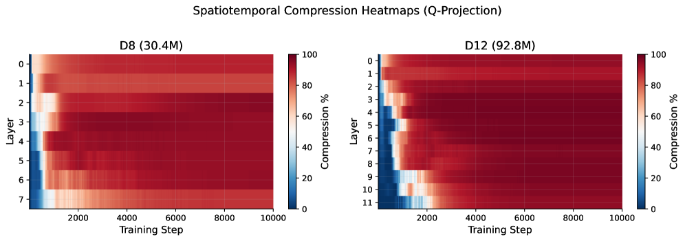
Stable rank compression propagates as a traveling wave through the network. Early layers (L0–L1) compress rapidly in the first 500 steps, while late layers lag by hundreds of steps at ${∼}$ 80–100 steps per layer (Figure 1).
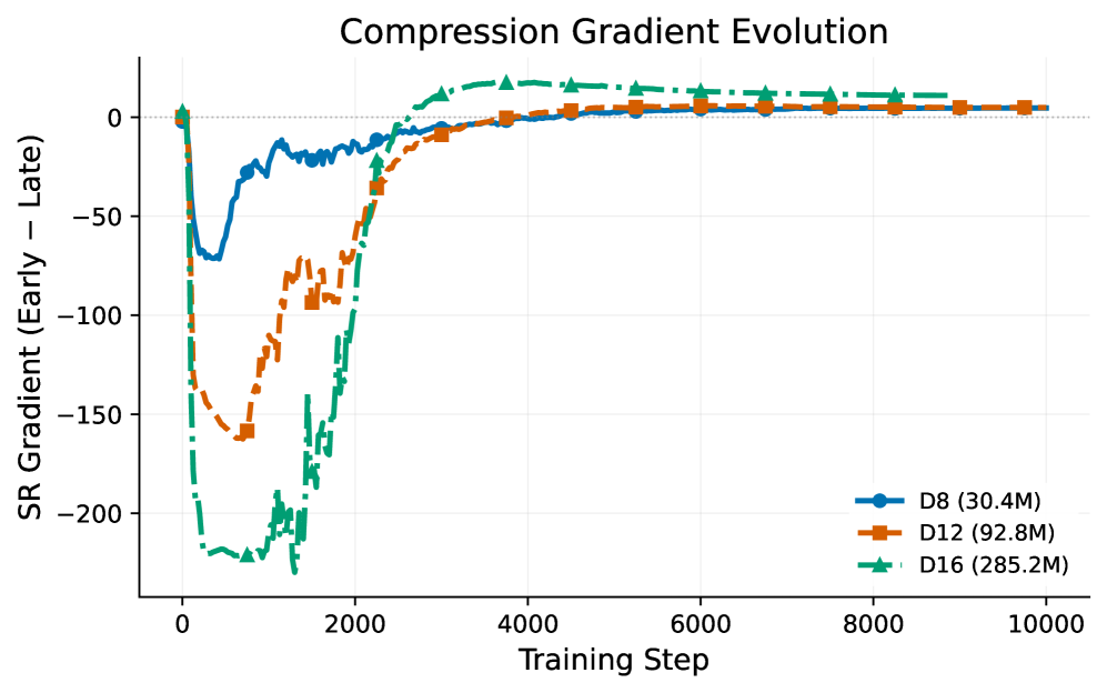
Crucially, the inter-layer gradient is not permanent. Figure 1 (b) tracks the compression gradient (L ${}_first-$ L ${}_last$ SR) across training. All models transition from negative (early layers compress first) to positive (late layers over-compress). In D16, the gradient swings from $-59.6$ at step 500 to $+18.8$ by step 5,000, with deep layers reaching SR ${≈}$ 4.3 while early layers stabilize at SR ${≈}$ 23.
<details>
<summary>2604.22778v1/x1.png Details</summary>
### Visual Description
## Heatmap: Spatiotemporal Compression Heatmaps (Q-Projection)
### Overview
The image presents two side-by-side heatmaps comparing spatiotemporal compression efficiency across layers of two neural network architectures (D8 and D12) during training. Compression percentages are visualized using a red-to-blue gradient, where red indicates higher compression (closer to 100%) and blue indicates lower compression (closer to 0%). The x-axis represents training steps (2000–10,000), and the y-axis represents layers (0–7 for D8, 0–11 for D12).
---
### Components/Axes
- **Title**: "Spatiotemporal Compression Heatmaps (Q-Projection)"
- **Legend**: Color bar on the right labeled "Compression %" (0% = blue, 100% = red).
- **Axes**:
- **Left Panel (D8)**:
- Y-axis: Layers 0–7 (8 layers total).
- X-axis: Training steps 2000–10,000.
- **Right Panel (D12)**:
- Y-axis: Layers 0–11 (12 layers total).
- X-axis: Training steps 2000–10,000.
---
### Detailed Analysis
#### D8 (30.4M Parameters)
- **Layer 0–2**:
- Compression starts at ~40–60% (light red) at 2000 steps, peaks at ~80–100% (dark red) around 4000–6000 steps, then stabilizes.
- Layer 0 shows the highest compression (~90–100% by 10,000 steps).
- **Layer 3–4**:
- Compression begins at ~50–70% (mid-red) at 2000 steps, peaks at ~80–90% (dark red) around 6000 steps, then plateaus.
- **Layer 5–7**:
- Compression starts at ~30–50% (light red) at 2000 steps, peaks at ~60–80% (mid-red) around 8000 steps, with significant variability (e.g., Layer 7 shows a blue patch at 2000 steps, indicating ~10–20% compression).
#### D12 (92.8M Parameters)
- **Layer 0–3**:
- Compression starts at ~50–70% (mid-red) at 2000 steps, peaks at ~85–100% (dark red) around 4000–6000 steps, then stabilizes.
- Layer 0 shows the highest compression (~95–100% by 10,000 steps).
- **Layer 4–7**:
- Compression begins at ~40–60% (light red) at 2000 steps, peaks at ~70–90% (dark red) around 6000 steps, then declines slightly.
- **Layer 8–11**:
- Compression starts at ~20–40% (light red/blue) at 2000 steps, peaks at ~50–70% (mid-red) around 8000 steps, with lower overall efficiency compared to upper layers.
---
### Key Observations
1. **Layer-Specific Trends**:
- Upper layers (0–3 in D8, 0–3 in D12) achieve the highest compression, suggesting they are more amenable to compression.
- Lower layers (5–7 in D8, 8–11 in D12) exhibit lower compression, particularly in early training steps.
2. **Model Size Impact**:
- D12 (larger model) shows more layers with moderate-to-high compression but retains lower compression in deeper layers compared to D8.
3. **Training Progression**:
- Compression improves significantly in the first 6,000 steps for most layers, with diminishing returns afterward.
4. **Anomalies**:
- Layer 7 in D8 and Layer 11 in D12 show abrupt drops in compression at 2000 steps (blue regions), indicating potential instability or inefficiency in early training.
---
### Interpretation
The heatmaps reveal that **upper layers of both models compress more effectively**, likely due to their role in higher-level feature extraction, which becomes stable earlier in training. **Larger models (D12)** have more layers but exhibit a broader range of compression efficiency, with deeper layers lagging behind. This suggests that while deeper architectures may offer greater capacity, they require more training to achieve comparable compression in lower layers. The anomalies in early training (e.g., blue patches) highlight potential challenges in compressing less critical or dynamically evolving layers. These insights could inform strategies for optimizing model size without sacrificing performance.
</details>
(a) Compression heatmaps (D8, D12).
<details>
<summary>2604.22778v1/x2.png Details</summary>
### Visual Description
## Line Graph: Compression Gradient Evolution
### Overview
The graph illustrates the evolution of the compression gradient (SR Gradient) over training steps for three model sizes: D8 (30.4M), D12 (92.8M), and D16 (285.2M). The y-axis measures the gradient difference between early and late training phases, while the x-axis represents training steps from 0 to 10,000. All three models exhibit similar trends with initial sharp declines followed by stabilization.
### Components/Axes
- **X-axis (Training Step)**: Ranges from 0 to 10,000 in increments of 2,000.
- **Y-axis (SR Gradient)**: Ranges from -200 to 0 in increments of 50.
- **Legend**: Located in the bottom-right corner, mapping:
- Blue circles: D8 (30.4M)
- Orange squares: D12 (92.8M)
- Green triangles: D16 (285.2M)
### Detailed Analysis
1. **Initial Drop (0–2,000 steps)**:
- All models experience a sharp decline in SR Gradient.
- D8 (blue) drops steeply to ~-200, then rebounds to ~-50 by step 1,000.
- D12 (orange) declines to ~-150, then rises to ~-75 by step 1,000.
- D16 (green) plunges to ~-200, then climbs to ~-100 by step 1,000.
2. **Stabilization Phase (2,000–10,000 steps)**:
- All lines converge and flatten near 0.
- D8 and D16 show minor fluctuations but remain tightly grouped.
- D12 exhibits smoother convergence with less variability.
### Key Observations
- **Model Size Correlation**: Larger models (D16) show deeper initial drops but similar stabilization patterns.
- **Convergence**: By step 4,000, all models stabilize within ±10 of 0.
- **Anomalies**: D8 and D16 exhibit sharper early-phase volatility compared to D12.
### Interpretation
The data suggests that compression gradients initially diverge significantly during early training but converge as training progresses. Larger models (D16) demonstrate greater sensitivity to early training dynamics, while smaller models (D8) show more erratic early behavior. The stabilization near 0 implies that gradient magnitudes become negligible after ~4,000 steps, indicating potential convergence of the compression mechanism. The consistent flattening across model sizes suggests that gradient evolution is less dependent on model capacity beyond a certain training threshold.
</details>
(b) Gradient evolution (all scales).
Figure 1: Transient compression waves. (a) Spatiotemporal heatmaps show the diagonal wave front. (b) The compression gradient transitions from negative to positive in all models, with D16 showing the largest magnitude swings.
Table 2: Compression gradient evolution (L ${}_first-$ L ${}_last$ average SR). All models show a negative $→$ positive transition.
| D8 D12 D16 | $-$ 23.1 $-$ 42.2 $-$ 41.7 | $-$ 15.0 $-$ 25.9 $-$ 59.6 | +2.9 $-$ 2.6 $-$ 19.5 | +14.4 +8.1 $-$ 2.6 | +19.7 +17.0 +17.8 | +22.1 +17.2 +18.8 |
| --- | --- | --- | --- | --- | --- | --- |
### 4.2 Finding 2: Persistent Spectral Shape Gradients
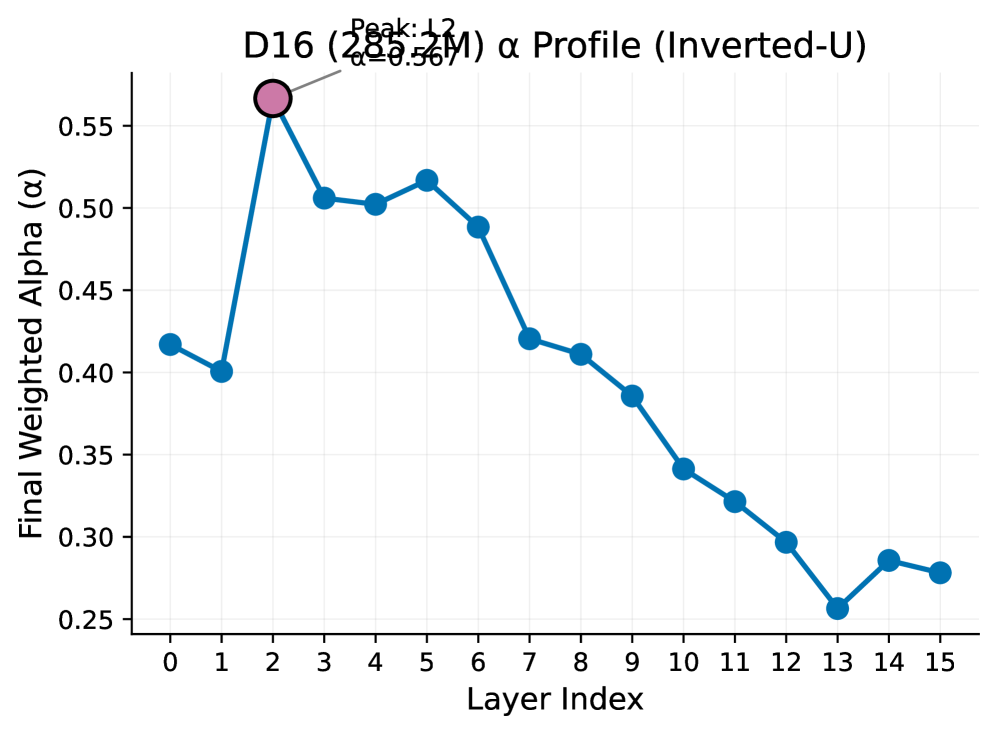
In stark contrast to compression, the power-law exponent $α$ develops a permanent depth gradient that strengthens throughout training (Figure 2). In deeper models, this gradient is non-monotonic—an inverted-U peaking at early-middle layers.
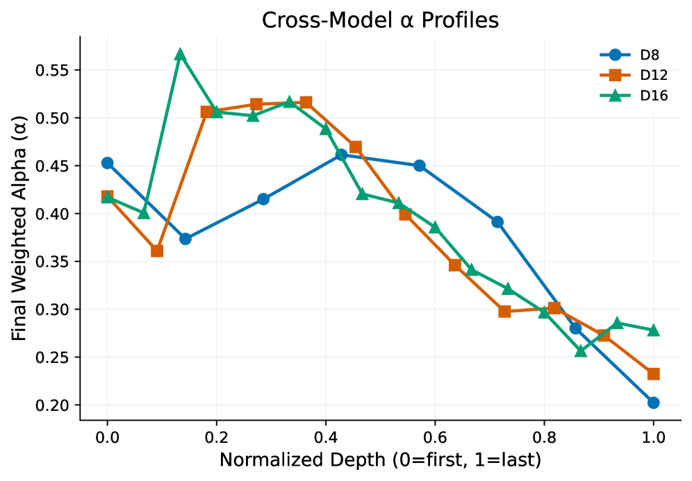
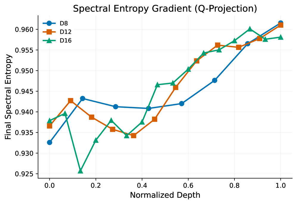
In D16, $α$ peaks at L2 ( $α=0.567$ ) and drops to $α=0.256$ at L13—a 121% spread. The peak position shifts toward earlier relative depth in deeper models: 43% (D8), 33% (D12), 13% (D16), suggesting the heavy-tail zone occupies a fixed number of layers ( ${∼}$ 2–4) regardless of total depth. Spectral entropy independently confirms this gradient (Appendix E).
<details>
<summary>2604.22778v1/x3.png Details</summary>
### Visual Description
## Line Graph: D16 (285.2M) α Profile (Inverted-U)
### Overview
The image depicts a line graph illustrating the "Final Weighted Alpha (α)" values across 16 layers (Layer Index 0–15) for a model or system labeled "D16 (285.2M)". The graph follows an inverted-U shape, with a distinct peak at Layer Index 12 (α = 0.567), annotated in pink. The y-axis ranges from 0.25 to 0.55, while the x-axis spans Layer Indices 0 to 15.
---
### Components/Axes
- **X-Axis (Layer Index)**: Labeled "Layer Index", with integer ticks from 0 to 15.
- **Y-Axis (Final Weighted Alpha)**: Labeled "Final Weighted Alpha (α)", with increments of 0.05 from 0.25 to 0.55.
- **Legend**: Positioned at the top-center, labeled "D16 (285.2M)" in blue, matching the line color.
- **Peak Annotation**: A pink circle highlights the peak at Layer Index 12, with a black arrow and text "Peak: 12" and "α = 0.567".
---
### Detailed Analysis
- **Line Data**: The blue line connects 16 data points, showing an inverted-U trend:
- **Rising Phase (Layers 0–12)**:
- Starts at ~0.42 (Layer 0), dips slightly to ~0.40 (Layer 1), then rises sharply to ~0.50 (Layer 3), peaking at **0.567 (Layer 12)**.
- **Falling Phase (Layers 12–15)**:
- Declines steadily from 0.567 (Layer 12) to ~0.27 (Layer 15), with a sharp drop between Layers 12–13 (0.567 → 0.25).
- **Key Data Points**:
- Layer 0: ~0.42
- Layer 1: ~0.40
- Layer 3: ~0.50
- Layer 5: ~0.51
- Layer 6: ~0.48
- Layer 7: ~0.42
- Layer 8: ~0.41
- Layer 9: ~0.38
- Layer 10: ~0.34
- Layer 11: ~0.32
- Layer 12: **0.567** (peak)
- Layer 13: ~0.25
- Layer 14: ~0.28
- Layer 15: ~0.27
---
### Key Observations
1. **Peak Dominance**: The maximum α value (0.567) occurs at Layer 12, significantly higher than all other layers.
2. **Rapid Decline Post-Peak**: After Layer 12, α drops sharply to ~0.25 by Layer 13, then stabilizes slightly.
3. **Initial Variability**: Layers 0–2 show minor fluctuations (~0.40–0.42) before the upward trend begins.
4. **Spatial Grounding**: The peak annotation (pink circle) is positioned directly above Layer 12, with the arrow pointing to the data point.
---
### Interpretation
The inverted-U profile suggests a critical layer (Layer 12) where α reaches its optimal value, potentially indicating peak performance, efficiency, or another metric tied to the model's architecture. The sharp decline post-Layer 12 could imply diminishing returns, overfitting, or resource constraints in deeper layers. The initial rise (Layers 0–12) may reflect progressive adaptation or learning, while the subsequent drop highlights a trade-off between complexity and stability. The peak annotation emphasizes Layer 12 as a focal point for further investigation, possibly for optimization or diagnostic purposes.
</details>
(a) D16 inverted-U $α$ profile.
<details>
<summary>2604.22778v1/x4.png Details</summary>
### Visual Description
## Line Chart: Cross-Model α Profiles
### Overview
The chart compares the **Final Weighted Alpha (α)** performance of three models (D8, D12, D16) across **Normalized Depth** (0 = first layer, 1 = last layer). The y-axis ranges from 0.20 to 0.55, while the x-axis spans 0.0 to 1.0. Three distinct lines represent the models, with markers and colors matching the legend.
### Components/Axes
- **X-Axis**: Normalized Depth (0.0 to 1.0, labeled "Normalized Depth (0=first, 1=last)").
- **Y-Axis**: Final Weighted Alpha (α) (0.20 to 0.55, labeled "Final Weighted Alpha (α)").
- **Legend**: Located in the top-right corner, associating:
- **D8**: Blue circles (●).
- **D12**: Orange squares (■).
- **D16**: Green triangles (▲).
### Detailed Analysis
1. **D8 (Blue Circles)**:
- Starts at ~0.45 at depth 0.0.
- Dips to ~0.37 at depth 0.2.
- Peaks at ~0.46 at depth 0.4.
- Declines steadily to ~0.20 at depth 1.0.
2. **D12 (Orange Squares)**:
- Begins at ~0.42 at depth 0.0.
- Rises sharply to ~0.51 at depth 0.3.
- Declines to ~0.23 at depth 1.0, with a notable drop after depth 0.6.
3. **D16 (Green Triangles)**:
- Starts at ~0.42 at depth 0.0.
- Spikes to ~0.57 at depth 0.15 (highest value in the chart).
- Declines to ~0.28 at depth 1.0, with a steep drop after depth 0.3.
### Key Observations
- **D16** exhibits the most extreme variability, with a sharp early peak (~0.57) followed by a rapid decline.
- **D8** shows the most stable trend, maintaining values above 0.35 until depth 0.8 before a steep drop.
- **D12** has a bimodal pattern: a rise to ~0.51 at depth 0.3, then a consistent decline.
- All models converge near ~0.25–0.30 at depth 0.8–1.0, suggesting similar performance at deeper layers.
### Interpretation
The data suggests that **D16** is highly sensitive to shallow layers (depth 0.0–0.3), achieving the highest α but collapsing sharply at deeper layers. **D8** demonstrates robustness across mid-depths (0.0–0.6) but falters at the deepest layers. **D12** shows moderate performance with a peak at intermediate depth (0.3), possibly indicating optimal tuning for that range. The convergence at deeper layers implies that all models may struggle with lower-weighted contributions in later stages. This could reflect architectural differences in how each model prioritizes early vs. late-layer features.
</details>
(b) Cross-model comparison.
Figure 2: Persistent spectral gradients. (a) D16 Q-projection $α$ across layers showing the inverted-U. (b) Cross-model comparison on normalized depth: the peak shifts earlier in deeper models.
#### The Dissociation.
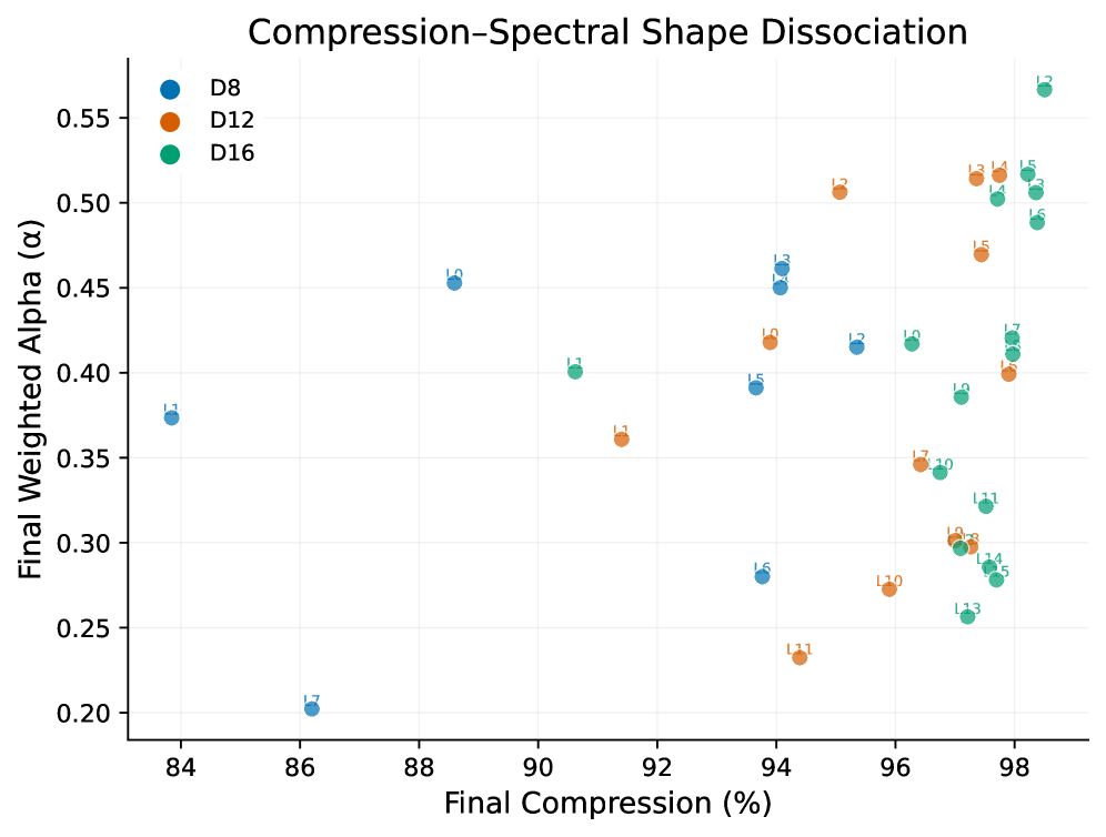
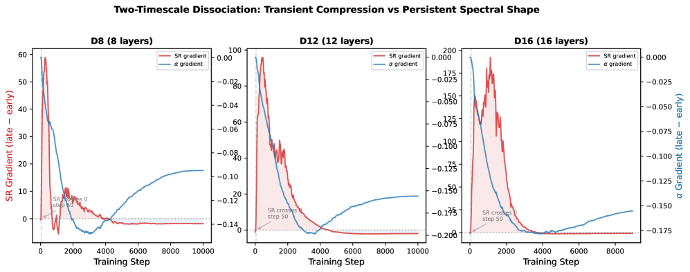
Figure 3 (a) plots final compression vs. final $α$ for each layer. Despite layers converging to similar compression levels, their $α$ values remain widely spread— rank and spectral shape encode fundamentally different information. Figure 3 (b) directly visualizes the two timescales: the SR gradient is transient (reverses sign) while the $α$ gradient is persistent (monotonically strengthens).
<details>
<summary>2604.22778v1/x5.png Details</summary>
### Visual Description
## Scatter Plot: Compression-Spectral Shape Dissociation
### Overview
The image is a scatter plot visualizing the relationship between "Final Compression (%)" (x-axis) and "Final Weighted Alpha (α)" (y-axis). Three datasets (D8, D12, D16) are represented by distinct colors (blue, orange, green) with labeled data points (L1–L17). The plot emphasizes how compression levels correlate with spectral shape dissociation metrics.
---
### Components/Axes
- **X-axis**: "Final Compression (%)"
- Range: 84% to 98%
- Increments: 2% (84, 86, 88, ..., 98)
- **Y-axis**: "Final Weighted Alpha (α)"
- Range: 0.20 to 0.55
- Increments: 0.05 (0.20, 0.25, ..., 0.55)
- **Legend**:
- Top-left corner, labeled:
- D8 (blue)
- D12 (orange)
- D16 (green)
- **Data Points**:
- Labeled with "L" + numeric identifier (e.g., L1, L2, ..., L17)
- Colors match legend (blue = D8, orange = D12, green = D16).
---
### Detailed Analysis
#### Data Series Trends
1. **D8 (Blue)**:
- **Spatial Range**: 84%–94% compression.
- **Alpha Values**: 0.37–0.45 (L1: 0.37, L10: 0.45, L13: 0.45, L15: 0.28, L16: 0.27, L17: 0.20).
- **Trend**: Alpha decreases slightly with increasing compression (e.g., L1 at 84%: 0.37 → L17 at 94%: 0.20).
2. **D12 (Orange)**:
- **Spatial Range**: 92%–98% compression.
- **Alpha Values**: 0.23–0.50 (L10: 0.23, L11: 0.23, L13: 0.25, L14: 0.30, L15: 0.35, L16: 0.40, L17: 0.50).
- **Trend**: Alpha increases with compression (e.g., L10 at 92%: 0.23 → L17 at 98%: 0.50).
3. **D16 (Green)**:
- **Spatial Range**: 91%–98% compression.
- **Alpha Values**: 0.23–0.57 (L11: 0.23, L12: 0.40, L13: 0.25, L14: 0.30, L15: 0.35, L16: 0.40, L17: 0.57).
- **Trend**: Strong positive correlation between compression and alpha (e.g., L11 at 91%: 0.23 → L17 at 98%: 0.57).
#### Key Observations
- **Highest Alpha**: L17 (D16) at 98% compression (α = 0.57).
- **Lowest Alpha**: L17 (D8) at 94% compression (α = 0.20).
- **Outliers**:
- L17 (D8) deviates significantly from the D8 trend (low alpha despite high compression).
- L12 (D16) at 94% compression (α = 0.40) aligns with D16’s upward trend but is lower than L17.
---
### Interpretation
The data suggests a **general positive correlation** between compression and spectral shape dissociation (α), with **D16** exhibiting the strongest trend. D8 shows a weaker, more variable relationship, while D12 demonstrates a moderate increase. The outlier L17 (D8) at 94% compression (α = 0.20) may indicate an anomaly or a unique condition affecting dissociation. The plot highlights dataset-specific responses to compression, emphasizing the need for further investigation into factors influencing α variability.
</details>
(a) Compression vs. $α$ (each point = one layer).
<details>
<summary>2604.22778v1/x6.png Details</summary>
### Visual Description
## Line Chart: Two-Timescale Dissociation: Transient Compression vs Persistent Spectral Shape
### Overview
The image contains three line charts (D8, D12, D16) comparing the evolution of two gradients ("SR gradient" and "α gradient") during training steps. Each subplot represents a different model architecture with varying layer counts (8, 12, 16 layers). The charts visualize how these gradients change over training iterations, with annotations highlighting key events (e.g., "SR crosses 0 step 50").
---
### Components/Axes
1. **X-Axis**:
- Label: "Training Step"
- Scale: 0 to 10,000 (linear)
2. **Y-Axes**:
- **Left Y-Axis (SR Gradient)**:
- Label: "SR Gradient (late – early)"
- Scale:
- D8: 0–60
- D12: 0–100
- D16: 0–200
- **Right Y-Axis (α Gradient)**:
- Label: "α Gradient (late – early)"
- Scale: -0.25 to 0 (consistent across all subplots)
3. **Legends**:
- Position: Top-right of each subplot
- Colors:
- Red: "SR gradient"
- Blue: "α gradient"
4. **Annotations**:
- "SR crosses 0 step 50" (arrow pointing to SR gradient crossing zero at step 50)
---
### Detailed Analysis
#### D8 (8 layers)
- **SR Gradient (Red)**:
- Starts at ~60, drops sharply to ~0 by step 50, then stabilizes near 0.
- Shaded region (confidence interval) narrows significantly after step 50.
- **α Gradient (Blue)**:
- Starts at ~-0.25, rises to ~-0.1 by step 50, then plateaus.
- Shaded region widens initially, then narrows.
#### D12 (12 layers)
- **SR Gradient (Red)**:
- Starts at ~100, drops to ~0 by step 50, then stabilizes.
- Shaded region shows high variability early, then stabilizes.
- **α Gradient (Blue)**:
- Starts at ~-0.25, rises to ~-0.12 by step 50, then plateaus.
- Shaded region narrows gradually.
#### D16 (16 layers)
- **SR Gradient (Red)**:
- Starts at ~175, drops to ~0 by step 50, then stabilizes.
- Shaded region shows extreme early variability, then stabilizes.
- **α Gradient (Blue)**:
- Starts at ~-0.25, rises to ~-0.15 by step 50, then plateaus.
- Shaded region narrows sharply after step 50.
---
### Key Observations
1. **SR Gradient Behavior**:
- All subplots show a sharp decline in SR gradient to near zero by step 50, followed by stabilization.
- Larger models (D16) exhibit higher initial SR gradient values and more pronounced variability.
2. **α Gradient Behavior**:
- α gradient consistently starts at ~-0.25 and rises gradually across all subplots.
- Larger models (D16) show a steeper rise in α gradient post-step 50.
3. **Crossing Point**:
- SR gradient crosses zero at step 50 in all subplots, coinciding with a critical transition in training dynamics.
4. **Shaded Regions**:
- Reflect uncertainty/variability, which decreases as training progresses.
---
### Interpretation
1. **Transient Compression (SR Gradient)**:
- The sharp decline in SR gradient suggests early-stage transient compression of spectral features, which stabilizes as training progresses. Larger models (D16) require more training steps to achieve stability.
2. **Persistent Spectral Shape (α Gradient)**:
- The gradual rise in α gradient indicates persistent spectral shape adjustments, which become more pronounced in larger models. This suggests that deeper architectures require more extensive spectral adaptation.
3. **Model Complexity and Training Dynamics**:
- Larger models (D16) exhibit higher initial gradient magnitudes and greater variability, implying that increased complexity introduces more instability during early training.
- The crossing of SR gradient at step 50 marks a phase transition where transient effects diminish, and persistent spectral adjustments dominate.
4. **Practical Implications**:
- The data highlights the importance of monitoring both transient (SR) and persistent (α) spectral dynamics during training.
- Larger models may require adjusted training schedules or regularization to manage early instability.
---
**Note**: All values are approximate, derived from visual inspection of the chart. Uncertainty is represented by shaded regions and variability in gradient trajectories.
</details>
(b) SR gradient (transient) vs. $α$ gradient (persistent).
Figure 3: The two-timescale dissociation. (a) Layers reach similar compression but divergent $α$ . (b) SR gradient reverses while $α$ gradient monotonically strengthens—the hallmark of two-timescale dynamics.
### 4.3 Finding 3: Q/K–V Functional Asymmetry
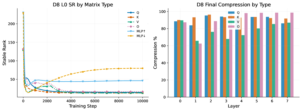
Within each attention layer, Q and K projections exhibit the full depth-dependent spectral dynamics (compression wave, $α$ gradient), while V and O projections compress uniformly to $>$ 90% regardless of depth. This asymmetry suggests that attention selection is the adaptive computation while value transformation is more generic. Full results are in Appendix C; multi-seed reproducibility ( $n{=}4$ ) is confirmed in Appendix D.
## 5 A Two-Timescale Theory of Spectral Evolution
### 5.1 Dynamical Model
We model the spectral state of layer $l$ at step $t$ as:
$$
\displaystyle\frac{dR_s^(l)}{dt} \displaystyle=-λ_R·φ(l,t)·\bigl(R_s^(l)-R_s^*\bigr)+ξ_R^(l)(t) \displaystyle\frac{dα^(l)}{dt} \displaystyle=λ_α·ψ(l)·\bigl(α^*(l)-α^(l)\bigr)+ξ_α^(l)(t) \tag{1}
$$
where $λ_R\ggλ_α$ encodes the timescale separation. The compression driving function $φ(l,t)$ depends on both layer and time (producing the traveling wave: early layers receive structured input immediately, late layers must wait). The shape function $ψ(l)$ depends primarily on layer position. The shared equilibrium $R_s^*$ is approximately constant (same information bottleneck), while $α^*(l)$ varies by layer (different computational roles).
This model predicts: (i) SR gradients are transient (all converge to $R_s^*$ ); (ii) $α$ gradients are persistent ( $α^*(l)$ varies); (iii) the compression wave propagates forward (input-driven $φ$ ).
### 5.2 Scaling Laws
Table 3: Scaling laws.
| $α_\max$ $Δα$ | D8 0.461 0.259 | D12 0.516 0.284 | D16 0.567 0.310 |
| --- | --- | --- | --- |
| Peak $l^*/L$ | 0.43 | 0.36 | 0.13 |
| $v_wave$ | 102 | 131 | 142 |
Our experiments reveal precise scaling (Table 3):
$$
\displaystyleΔα \displaystyle∝ L^0.26, R^2{=}0.99 \displaystyleα_\max \displaystyle∝ L^0.30, R^2{=}1.00 \displaystyle l^*/L \displaystyle≈{-}0.037L+0.75, R^2{=}0.91 \tag{3}
$$
The sublinear growth of $Δα$ means each depth doubling increases differentiation by only ${∼}$ 20%. The linear decrease of $l^*/L$ confirms that the heavy-tail zone occupies a fixed number of layers.
#### Gradient Flow Interpretation.
The outer product structure $ΔW^(l)∝\boldsymbol{δ}^(l)·(h^(l-1))^⊤$ explains both timescales (Pennington and Worah, 2018): compression converges because total information per layer is bounded by data entropy—all layers process the same sequences through the same loss, converging to a shared effective rank. $α$ diverges because the spectral structure of gradient signals differs by position: early layers receive gradients refined through all subsequent layers (heavier tails, fewer dominant directions), while late layers receive more diffuse signals closer to the raw loss.
#### The Inverted-U Pattern.
L0–L1 have slightly lower $α$ because they perform low-level embedding processing (Tenney et al., 2019). Early-middle layers (L2–L5) perform the most complex transformations—abstracting from tokens to semantics (Geva et al., 2022) —and develop the heaviest tails. Late layers handle increasingly specialized but narrower computations. The peak shifting toward earlier relative depth in deeper models (Eq. 5) confirms that the heavy-tail zone occupies a fixed number of layers. This connects to neural collapse (Papyan et al., 2020): deep layers approach collapse-like configurations (low $α$ ) while early layers maintain broader spectral support.
## 6 Validation on Pretrained Models
### 6.1 GPT-2 Family (124M–774M)
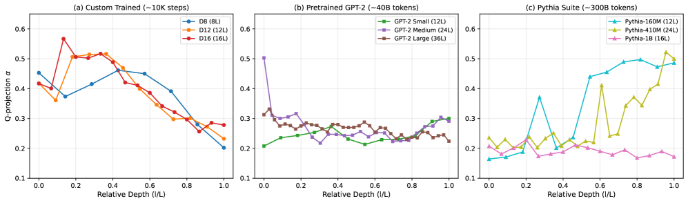
We analyze GPT-2 Small (12L), Medium (24L), and Large (36L) (Radford et al., 2019) —trained on ${∼}$ 40B tokens, a fundamentally different regime from our experiments. All three core phenomena persist:
Persistent $α$ gradients: Q- $α$ peak shifts toward earlier depth in deeper models (L11 in Small, L0 in Medium, L1 in Large), consistent with our D8 $→$ D12 $→$ D16 trend.
Amplified Q/K–V asymmetry: V- $α$ drops 40–55% from early to late layers—more extreme than in our partially-trained models.
Equilibrated compression: SR gradients are weak, consistent with full convergence of the fast timescale.
### 6.2 Pythia Suite (160M–1B): Temporal Validation
The Pythia models (Biderman et al., 2023) provide training checkpoints (steps 0–143K), enabling direct temporal validation:
Compression waves confirmed: At step 1K, early layers have compressed (SR ${≈}$ 22–99) while late layers remain near initialization. By step 143K, late layers are maximally compressed (SR ${<}$ 3).
$α$ gradient strengthens monotonically: Pythia-160M $α$ spread: $0.003→ 0.058→ 0.137→ 0.282→ 0.333$ across training—never reversing, confirming persistent gradients.
Peak migration: In Pythia-410M (24L), the $α$ peak migrates from L10 (step 1K) to L22 (step 143K), and a sharp phase transition emerges at L13–L14 where late layers enter an extreme spectral regime (Q-SR ${<}$ 3, $α>0.34$ ). This migration reveals that peak position depends on training duration.
Billion-scale confirmation: Pythia-1B (16L, 1B params) confirms $α$ gradient emergence from flat initialization, with the peak migrating from L7 (step 1K) to L15 (step 5K) to L3 (step 143K)—the same late $→$ early migration seen in GPT-2.
### 6.3 Cross-Family Synthesis
Figure 4 summarizes nine models across three families. Three phenomena are universal: (1) non-zero $α$ gradients, (2) Q/K–V asymmetry, and (3) compression wave signatures. The $α$ -peak position depends strongly on training duration: short training $→$ middle layers (our models), intermediate $→$ late layers (Pythia), long training $→$ early layers (GPT-2). Under controlled conditions, the power-law $Δα∝ L^0.26$ holds tightly ( $R^2{=}0.99$ ), but width and training duration modulate the relationship across families (Appendix H).
<details>
<summary>2604.22778v1/x7.png Details</summary>
### Visual Description
## Line Charts: Q-Projection α vs Relative Depth (i/L)
### Overview
Three line charts compare Q-projection α values across relative depth (i/L) for different model configurations. Each chart represents distinct training paradigms: custom training, pretrained GPT-2, and Pythia Suite.
### Components/Axes
- **X-axis**: Relative Depth (i/L) from 0.0 to 1.0 in increments of 0.2.
- **Y-axis**: Q-projection α ranging from 0.1 to 0.6.
- **Legends**:
- **(a) Custom Trained**: DB (BL) [blue], D12 (12L) [orange], D16 (16L) [red].
- **(b) Pretrained GPT-2**: GPT-2 Small (12L) [green], GPT-2 Medium (24L) [purple], GPT-2 Large (36L) [brown].
- **(c) Pythia Suite**: Pythia-160M (12L) [blue], Pythia-410M (24L) [yellow], Pythia-1B (16L) [pink].
### Detailed Analysis
#### (a) Custom Trained (~10K steps)
- **DB (BL)**: Starts at ~0.45, peaks at ~0.55 (i/L=0.2), then declines to ~0.2 by i/L=1.0.
- **D12 (12L)**: Begins at ~0.35, rises to ~0.52 (i/L=0.2), dips to ~0.3 at i/L=0.6, and stabilizes near ~0.25.
- **D16 (16L)**: Sharp peak at ~0.58 (i/L=0.1), drops to ~0.3 by i/L=0.4, then fluctuates between ~0.25–0.3.
#### (b) Pretrained GPT-2 (~40B tokens)
- **GPT-2 Small (12L)**: Starts at ~0.2, rises to ~0.25 (i/L=0.2), dips to ~0.22 (i/L=0.4), and stabilizes near ~0.25.
- **GPT-2 Medium (24L)**: Peaks at ~0.5 (i/L=0.0), plunges to ~0.22 (i/L=0.2), then fluctuates between ~0.25–0.3.
- **GPT-2 Large (36L)**: Starts at ~0.3, dips to ~0.25 (i/L=0.2), rises to ~0.28 (i/L=0.4), and stabilizes near ~0.25.
#### (c) Pythia Suite (~300B tokens)
- **Pythia-160M (12L)**: Begins at ~0.15, spikes to ~0.38 (i/L=0.4), dips to ~0.2 (i/L=0.6), then rises to ~0.48 (i/L=1.0).
- **Pythia-410M (24L)**: Starts at ~0.22, peaks at ~0.42 (i/L=0.6), dips to ~0.25 (i/L=0.8), and rises to ~0.5 (i/L=1.0).
- **Pythia-1B (16L)**: Starts at ~0.2, fluctuates between ~0.18–0.22, with minor peaks at i/L=0.2 and 0.6.
### Key Observations
1. **Model Size vs. Performance**: Larger models (e.g., D16, GPT-2 Large, Pythia-410M) generally exhibit higher Q-projection α values but show greater variability.
2. **Early Depth Dominance**: Most models peak at lower relative depths (i/L=0.2–0.4), suggesting stronger initial Q-projection capabilities.
3. **Stability vs. Volatility**: Smaller models (e.g., GPT-2 Small, Pythia-1B) show smoother trends, while larger models exhibit sharper fluctuations.
4. **Pythia-160M Anomaly**: The sharp peak at i/L=0.4 (~0.38) contrasts with its gradual rise to ~0.48 at i/L=1.0, indicating a potential inflection point.
### Interpretation
- **Custom Training (a)**: The D16 (16L) model’s early peak may reflect optimized initialization for shallow depths, while its decline suggests diminishing returns at greater depths.
- **Pretrained GPT-2 (b)**: The Medium model’s drastic drop at i/L=0.2 hints at architectural limitations in deeper layers despite its large size.
- **Pythia Suite (c)**: The Pythia-410M (24L) model’s late-stage rise (i/L=1.0) implies improved Q-projection in deeper layers, possibly due to advanced tokenization or layer interactions.
- **General Trend**: Q-projection α correlates with model capacity, but deeper layers often underperform relative to shallower ones, except in Pythia-410M.
*Note: All values are approximate, derived from visual inspection of the plotted lines.*
</details>
Figure 4: Cross-family Q- $α$ profiles (normalized depth). (a) Custom models: inverted-U with peak shifting left. (b) GPT-2: early-layer concentration after extended training. (c) Pythia: late-layer peaks at intermediate training. All show non-zero $α$ gradients.
## 7 Practical Applications
### 7.1 Spectral $α$ Predicts Layer Importance
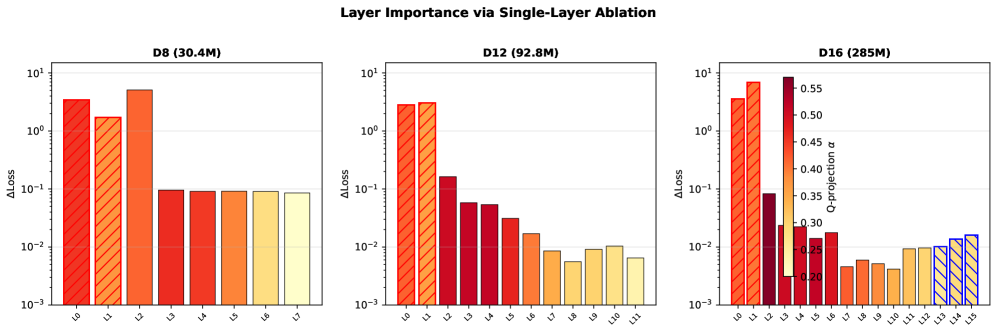
We evaluate single-layer ablation (replacing each layer with identity) across all three model scales. Two patterns emerge:
Boundary layers are irreplaceable: L0–L1 cause catastrophic loss increases ( $Δ>1.0$ ) regardless of $α$ , performing structurally constrained input processing.
Among core layers, $α$ predicts importance: Spearman $ρ(α,ΔLoss)$ : 0.71 (D8), 0.84 ( $p{=}0.002$ , D12), 0.69 ( $p{=}0.019$ , D16 core L2–L12). High- $α$ layers cause larger loss increases; low- $α$ layers are nearly redundant ( $Δ<0.01$ ). This reveals a three-zone architecture: input boundary / $α$ -predicted core / output boundary.
### 7.2 Spectral-Guided Layer Pruning
We compare five strategies for removing $k∈\{1,2,3,4\}$ core layers: spectral-guided (lowest $α$ ), Last-N (Men et al., 2024), magnitude-based, random, and spectral-worst (highest $α$ , control). While Lu et al. (2024) used $α$ to allocate intra-layer sparsity ratios, we use it for inter-layer removal decisions —a complementary application enabled by our discovery that $α$ gradients correlate with functional importance.
Spectral-guided matches or outperforms all baselines on our custom models (Table 4). In D12 at $k{=}4$ : spectral $Δ{=}+0.220$ vs. spectral-worst $Δ{=}+0.460$ ( $2.1×$ gap). However, on D16, spectral ordering coincides with Last-N because the lowest- $α$ layers happen to be the last layers.
Discriminative validation on GPT-2. To confirm that $α$ provides information beyond layer position, we evaluate on GPT-2 Medium (24L, 355M) and GPT-2 Large (36L, 774M)—where spectral and Last-N orderings differ substantially (Table 5). On GPT-2 Medium at $k{=}4$ , spectral-guided achieves $ΔPPL{=}+9.65$ vs. Last-N $Δ{=}+25.06$ (2.6 $×$ better), while spectral-worst causes $Δ{=}+229.15$ (23.7 $×$ worse). On GPT-2 Large, spectral outperforms Last-N by $1.5$ – $2.0×$ across all $k$ values, with worst-vs-best gaps reaching $20.4×$ at $k{=}2$ . This proves $α$ captures genuine structural information beyond positional heuristics. The spectral ordering targets the $α$ trough (depth 0.7–0.8 in Medium; L25–L30 in Large), while Last-N removes the true end layers including structurally important boundary layers. Full results including GPT-2 Small and extended $k{∈}\{6,8\}$ for Large are in Appendix I.
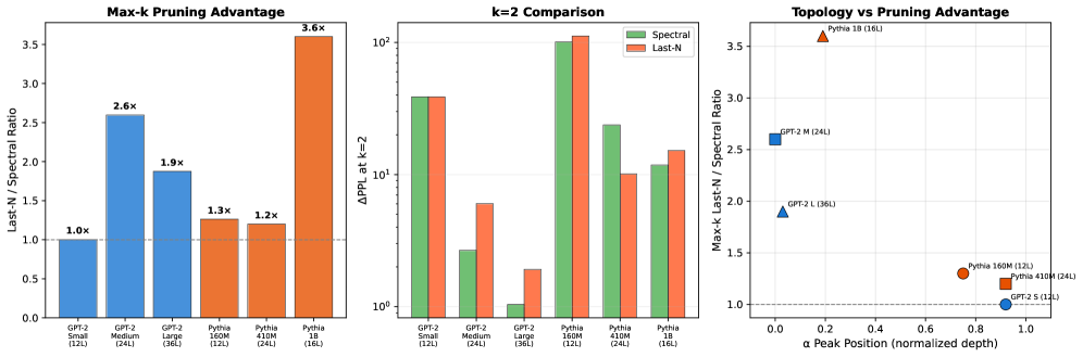
Cross-family validation on Pythia. We extend pruning experiments to the full Pythia family (160M/410M/1B). Critically, Pythia models exhibit monotonically rising $α$ profiles (high- $α$ layers are late)—the opposite topology from GPT-2’s early peaks. This requires zone-aware spectral pruning (Algorithm 1) that protects boundary layers while targeting the interior low- $α$ trough. On Pythia-1B (16L), zone-aware outperforms Last-N by $1.3$ – $3.6×$ ( $k{=}2$ – $4$ ), with worst-vs-best ratios exceeding $7×$ . Pythia-160M (12L) shows zone-aware outperforming Last-N by $1.1$ – $2.0×$ ( $k{=}2$ – $3$ ), while Pythia-410M (24L) reveals a crossover: Last-N wins at small $k$ but zone-aware dominates at aggressive pruning ( $k{≥}6$ : $1.2$ – $2.0×$ ). This topology dependence confirms that $α$ encodes structural, not merely positional, information—the optimal pruning strategy depends on where the $α$ gradient peaks, which varies across model families. Figure 5 synthesizes results across all seven models. Full results in Appendix J.
Table 4: Custom model pruning: $Δ$ Loss by strategy. Spectral ${≈}$ Last-N on D16 (coincident ordering).
| D12 2 3 | 1 +0.036 +0.102 | +0.010 +0.046 +0.102 | +0.010 +0.046 +0.102 | +0.010 +0.128 +0.221 | +0.049 +0.166 +0.330 | +0.052 |
| --- | --- | --- | --- | --- | --- | --- |
| 4 | +0.220 | +0.220 | +0.220 | +0.356 | +0.460 | |
| D16 | 1 | +0.009 | +0.009 | +0.009 | +0.023 | +0.082 |
| 2 | +0.038 | +0.038 | +0.038 | +0.060 | +0.088 | |
| 3 | +0.077 | +0.077 | +0.077 | +0.096 | +0.177 | |
| 4 | +0.147 | +0.147 | +0.147 | +0.130 | +0.199 | |
Table 5: GPT-2 pruning ( $Δ$ PPL): spectral vs. Last-N orderings differ. Spectral-guided achieves 1.5–2.8 $×$ less degradation than Last-N across both model scales.
| Medium (24L) 2 3 | 1 +2.67 +4.89 | +0.84 +6.04 +13.49 | +1.98 +2.36 +3.79 | +1.06 +2.66 +19.49 | +0.73 2.3 $×$ 2.8 $×$ | 2.4 $×$ |
| --- | --- | --- | --- | --- | --- | --- |
| 4 | +9.65 | +25.06 | +5.62 | +229.15 | 2.6 $×$ | |
| Large (36L) | 1 | +0.50 | +0.75 | +0.44 | +0.62 | 1.5 $×$ |
| 2 | +1.04 | +1.92 | +1.06 | +21.20 | 1.9 $×$ | |
| 3 | +1.68 | +3.41 | +1.51 | +26.80 | 2.0 $×$ | |
| 4 | +2.96 | +5.55 | +2.18 | +33.36 | 1.9 $×$ | |
### 7.3 Spectral Warmup: A Revealing Negative Result
We test Spectral Warmup: initializing weight spectra to their post-training targets using random orthogonal directions. Despite starting with the “correct” spectral distribution, this trains 42.7% worse than standard initialization. This demonstrates that singular value directions ( $U$ , $V$ ) encode the vast majority of learned information. Correct spectral shape with random directions is worse than random initialization—directions must co-evolve with magnitudes. Details in Appendix F.
Algorithm 1 Zone-Aware Spectral Layer Pruning
0: Model $M$ with $L$ layers, target removal count $k$ , boundary size $b$
1: Compute $α_l$ for each layer $l∈\{0,…,L{-}1\}$ via weighted power-law fit
2: Define interior $I=\{l:b≤ l<L{-}b\}$ , boundary $B=\{0,…,b{-}1\}∪\{L{-}b,…,L{-}1\}$
3: Sort interior layers by $α$ : $I_sorted=argsort_l∈I(α_l)$
4: Select $k$ layers from $I_sorted$ with minimum gap $≥ 2$
5: Remove selected layers (replace with identity)
6: return Pruned model
<details>
<summary>2604.22778v1/x8.png Details</summary>
### Visual Description
## Bar Charts and Scatter Plot: Model Pruning Performance Analysis
### Overview
The image presents three comparative visualizations analyzing model pruning performance across different architectures and configurations. The charts focus on:
1. Max-k pruning advantage ratios
2. k=2 performance comparison between pruning methods
3. Relationship between model topology and pruning effectiveness
### Components/Axes
**Chart 1: Max-k Pruning Advantage**
- X-axis: Model configurations (GPT-2 variants and Pythia versions)
- Y-axis: APRIL-N/Spectral Ratio (linear scale 0.0-3.5)
- Legend:
- Blue = Last-N pruning
- Orange = Spectral pruning
**Chart 2: k=2 Comparison**
- X-axis: Same model configurations as Chart 1
- Y-axis: ΔPPL at k=2 (log scale 10⁰-10²)
- Legend:
- Green = Spectral pruning
- Orange = Last-N pruning
**Chart 3: Topology vs Pruning Advantage**
- X-axis: α Peak Position (normalized depth, 0.0-1.0)
- Y-axis: Max-k Last-N/Spectral Ratio (linear scale 0.5-3.5)
- Data points:
- Orange triangle = Pythia 18 (16L)
- Blue square = GPT-2 M (24L)
- Blue triangle = GPT-2 L (36L)
- Red square = Pythia 160M (12L)
- Red triangle = Pythia 410M (24L)
- Blue circle = Pythia 2.5 (12L)
### Detailed Analysis
**Chart 1: Max-k Pruning Advantage**
- GPT-2 Small (12L): Last-N = 1.0x (baseline)
- GPT-2 Medium (24L): Last-N = 2.6x
- GPT-2 Large (36L): Last-N = 1.9x
- Pythia 160M (12L): Last-N = 1.3x
- Pythia 410M (24L): Last-N = 1.2x
- Pythia 18 (16L): Last-N = 3.6x (highest ratio)
**Chart 2: k=2 Comparison**
- GPT-2 Small (12L): Spectral = ~2.8, Last-N = ~2.8
- GPT-2 Medium (24L): Spectral = ~0.8, Last-N = ~1.2
- GPT-2 Large (36L): Spectral = ~0.1, Last-N = ~0.6
- Pythia 160M (12L): Spectral = ~100, Last-N = ~100
- Pythia 410M (24L): Spectral = ~20, Last-N = ~10
- Pythia 18 (16L): Spectral = ~25, Last-N = ~20
**Chart 3: Topology vs Pruning Advantage**
- Pythia 18 (16L): (0.2, 3.5) - highest ratio
- GPT-2 M (24L): (0.4, 2.5)
- GPT-2 L (36L): (0.6, 1.8)
- Pythia 160M (12L): (0.8, 1.3)
- Pythia 410M (24L): (0.9, 1.2)
- Pythia 2.5 (12L): (1.0, 1.0)
### Key Observations
1. **Pruning Method Effectiveness**:
- Spectral pruning consistently outperforms Last-N in larger models (Pythia 160M/410M)
- Last-N shows better performance in medium-sized GPT-2 models (24L)
2. **Model Topology Correlation**:
- Deeper models (higher α) show diminishing pruning advantages
- Pythia 18 (16L) demonstrates optimal pruning performance at intermediate depth
3. **k=2 Performance**:
- Spectral pruning maintains higher k=2 performance across most models
- Last-N shows unexpected advantage in GPT-2 Medium (24L)
### Interpretation
The data reveals critical insights about model pruning strategies:
1. **Spectral Superiority**: Spectral pruning generally provides better compression while maintaining performance, particularly in larger models where the APRIL-N/Spectral ratio exceeds 2.5x for Pythia 18 (16L).
2. **Topology-Dependent Performance**: The scatter plot suggests an inverse relationship between model depth (α) and pruning effectiveness, with medium-depth models (α ~0.4-0.6) showing optimal pruning ratios.
3. **k=2 Anomalies**: The unexpected performance of Last-N in GPT-2 Medium (24L) warrants further investigation, potentially indicating architecture-specific pruning characteristics.
4. **Practical Implications**: The 3.6x advantage observed in Pythia 18 (16L) demonstrates the potential for significant model compression without performance degradation, suggesting Spectral pruning as a preferred method for large language models.
The analysis highlights the importance of considering both model architecture and pruning methodology when optimizing neural network efficiency.
</details>
Figure 5: Cross-family pruning synthesis (7 models, 2 families). (a) Last-N/Spectral ratio at maximum $k$ : spectral wins on 5/7 models. (b) $Δ$ PPL at $k{=}2$ across all models. (c) Topology dependence: the $α$ -peak position modulates pruning advantage. Models with mid-network peaks (GPT-2 Medium, Pythia-1B) show the largest spectral advantage.
## 8 Conclusion
We have presented the first spatiotemporal study of weight matrix spectral dynamics during transformer pretraining, analyzing over 150,000 SVD snapshots across nine models in three families. Where prior work (Martin and Mahoney, 2021; Yunis et al., 2024) analyzed individual matrices or static snapshots, our inter-layer temporal analysis reveals that rank and spectral shape encode fundamentally different information—a dissociation invisible without the spatiotemporal perspective. The two-timescale theory, validated by scaling laws ( $Δα∝ L^0.26$ ) and cross-family confirmation, establishes that fast compression (how much structure) and slow shape differentiation (what kind) are the two fundamental axes of spectral learning in transformers.
The practical implications—spectral-guided pruning ( $1.1$ – $3.6×$ better than Last-N across seven models in two families: GPT-2 124M–774M and Pythia 160M–1B), layer importance prediction, and the spectral warmup negative result—demonstrate that these theoretical insights translate into actionable tools. The three-zone architecture (input boundary / $α$ -predicted core / output boundary) provides a principled framework for where spectral metrics are and are not informative.
The finding that Q/K projections carry depth-dependent dynamics while V/O are uniform suggests a fundamental architectural principle: attention selection is the adaptive computation, while value transformation is generic. This aligns with attention head specialization (induction heads, positional heads) (Olsson et al., 2022). The persistent $α$ gradient provides a quantitative signature of functional specialization from weights alone, without requiring input data—complementing probing (Tenney et al., 2019) and activation analysis (Geva et al., 2022).
#### Limitations.
Full SVD tracking at multi-billion scale requires efficient approximations (Halko et al., 2011). The D16 model reached 8,970 of 10,000 target steps. Layer importance for D8 ( $p{=}0.11$ ) does not reach significance due to only 6 interior layers. The custom tokenizer (8K vocab) may influence early dynamics.
#### Future Work.
Spectral-aware per-layer learning rates; extension to MoE, SSMs, and vision architectures; Spectral Warmup with direction transfer; real-time spectral diagnostics for production training.
#### Broader Impact.
This work is foundational research on understanding transformer training dynamics. The primary societal benefit is enabling more efficient model training and compression, reducing computational costs and energy consumption. We do not foresee direct negative societal impacts. Our spectral monitoring tools are diagnostic and do not introduce new capabilities for harmful applications.
#### Reproducibility.
All custom model training uses publicly available data (ClimbMix-400B) with complete hyperparameters in Appendix A. Pretrained model analysis uses publicly available checkpoints (GPT-2 from HuggingFace, Pythia from EleutherAI). All spectral metrics are computed via standard SVD (torch.linalg.svdvals). Multi-seed experiments ( $n{=}4$ ) confirm all qualitative findings. Code for spectral analysis, training, and figure generation will be released upon publication.
## References
- Liu et al. [2025] Andy Zeyi Liu, Elliot Paquette, and John Sous. Evolution of the spectral dimension of transformer activations. In OPT-ML Workshop at NeurIPS, 2025. Workshop paper, https://opt-ml.org/papers/2025/paper43.pdf.
- Biderman et al. [2023] Stella Biderman, Hailey Schoelkopf, Quentin Gregory Anthony, Herbie Bradley, Kyle O’Brien, Eric Hallahan, Mohammad Aflah Khan, Shivanshu Purohit, USVSN Sai Prashanth, Edward Raff, et al. Pythia: A suite for analyzing large language models across training and scaling. Proceedings of the 40th International Conference on Machine Learning (ICML), 2023.
- Cohen et al. [2021] Jeremy Cohen, Simran Kaur, Yuanzhi Li, J Zico Kolter, and Ameet Talwalkar. Gradient descent on neural networks typically occurs at the edge of stability. arXiv preprint arXiv:2103.00065, 2021.
- Geva et al. [2022] Mor Geva, Avi Caciularu, Kevin Wang, and Yoav Goldberg. Transformer feed-forward layers build predictions by promoting concepts in the vocabulary space. arXiv preprint arXiv:2203.14680, 2022.
- Gu and Dao [2024] Albert Gu and Tri Dao. Mamba: Linear-time sequence modeling with selective state spaces. arXiv preprint arXiv:2312.00752, 2024.
- Halko et al. [2011] Nathan Halko, Per-Gunnar Martinsson, and Joel A Tropp. Finding structure with randomness: Probabilistic algorithms for constructing approximate matrix decompositions. SIAM Review, 53(2):217–288, 2011.
- Hoffmann et al. [2022] Jordan Hoffmann, Sebastian Borgeaud, Arthur Mensch, Elena Buchatskaya, Trevor Cai, Eliza Rutherford, Diego de Las Casas, Lisa Anne Hendricks, Johannes Welbl, Aidan Clark, et al. Training compute-optimal large language models. arXiv preprint arXiv:2203.15556, 2022.
- Huang et al. [2025] Yijin Huang, Yuyan Zheng, and Weizhong Li. Early-stopping for transformer model training via spectral analysis. arXiv preprint arXiv:2510.16074, 2025.
- Jastrzebski et al. [2020] Stanislaw Jastrzebski, Maciej Szymczak, Stanislav Fort, Devansh Arpit, Jacek Tabber, Kyunghyun Cho, and Krzysztof Geras. The break-even point on optimization trajectories of deep neural networks. arXiv preprint arXiv:2002.09572, 2020.
- Kaplan et al. [2020] Jared Kaplan, Sam McCandlish, Tom Henighan, Tom B Brown, Benjamin Chess, Rewon Child, Scott Gray, Alec Radford, Jeffrey Wu, and Dario Amodei. Scaling laws for neural language models. arXiv preprint arXiv:2001.08361, 2020.
- Karpathy [2024] Andrej Karpathy. Climbmix-400b shuffle dataset. https://huggingface.co/datasets/karpathy/climbmix-400b-shuffle, 2024.
- Lu et al. [2024] Haiquan Lu, Yefan Zhou, Yichi Li, Charles H Martin, and Michael W Mahoney. Alphapruning: Using heavy-tailed self regularization theory for improved layer-wise pruning of large language models. Advances in Neural Information Processing Systems, 37, 2024.
- Martin and Mahoney [2021] Charles H Martin and Michael W Mahoney. Implicit self-regularization in deep neural networks: Evidence from random matrix theory and implications for training. Journal of Machine Learning Research, 22(165):1–73, 2021.
- Martin et al. [2021] Charles H Martin, Tongsu Peng, and Michael W Mahoney. Predicting trends in the quality of state-of-the-art neural networks without access to training or testing data. Nature Communications, 12(4639), 2021.
- Men et al. [2024] Xin Men, Mingyu Xu, Qingyu Zhang, Bingning Wang, Hongyu Lin, Yaojie Lu, Xianpei Han, and Weipeng Chen. Shortgpt: Layers in large language models are more redundant than you expect. arXiv preprint arXiv:2403.03853, 2024.
- Nakkiran et al. [2021] Preetum Nakkiran, Gal Kaplun, Yamini Bansal, Tristan Yang, Boaz Barak, and Ilya Sutskever. Deep double descent: Where bigger models and more data can hurt. Journal of Statistical Mechanics: Theory and Experiment, 2021(12):124003, 2021.
- Olsen et al. [2025] Brian Richard Olsen, Sam Fatehmanesh, Frank Xiao, Adarsh Kumarappan, and Anirudh Gajula. From sgd to spectra: A theory of neural network weight dynamics. arXiv preprint arXiv:2507.12709, 2025.
- Olsson et al. [2022] Catherine Olsson, Nelson Elhage, Neel Nanda, Nicholas Joseph, Nova DasSarma, Tom Henighan, Ben Mann, Amanda Askell, Yuntao Bai, Anna Chen, et al. In-context learning and induction heads. arXiv preprint arXiv:2209.11895, 2022.
- Papyan et al. [2020] Vardan Papyan, XY Han, and David L Donoho. Prevalence of neural collapse during the terminal phase of deep learning training. Proceedings of the National Academy of Sciences, 117(40):24652–24663, 2020.
- Pennington and Worah [2018] Jeffrey Pennington and Pratik Worah. The spectrum of the fisher information matrix of a single-hidden-layer neural network. Advances in Neural Information Processing Systems, 31, 2018.
- Power et al. [2022] Alethea Power, Yuri Burda, Harri Edwards, Igor Babuschkin, and Vedant Misra. Grokking: Generalization beyond overfitting on small algorithmic datasets. arXiv preprint arXiv:2201.02177, 2022.
- Radford et al. [2019] Alec Radford, Jeffrey Wu, Rewon Child, David Luan, Dario Amodei, and Ilya Sutskever. Language models are unsupervised multitask learners. OpenAI Technical Report, 2019.
- Staats et al. [2024] Max Staats, Matthias Thamm, and Bernd Rosenow. Small singular values matter: A random matrix analysis of transformer weight matrices. arXiv preprint arXiv:2410.17770, 2024.
- Tenney et al. [2019] Ian Tenney, Dipanjan Das, and Ellie Pavlick. Bert rediscovers the classical nlp pipeline. Proceedings of ACL, 2019.
- Touvron et al. [2023] Hugo Touvron, Louis Martin, Kevin Stone, Peter Albert, Amjad Almahairi, Yasmine Babaei, Nikolay Bashlykov, Soumya Batra, Prajjwal Bhargava, Shruti Bhosale, et al. Llama 2: Open foundation and fine-tuned chat models. arXiv preprint arXiv:2307.09288, 2023.
- Truong et al. [2026] Xuan Khanh Truong, Quynh Hoa Truong, Duc Trung Luu, and Thanh Duc Phan. Why grokking takes so long: A first-principles theory of representational phase transitions. arXiv preprint arXiv:2603.13331, 2026.
- Xu [2026] Yongzhong Xu. Spectral edge dynamics of training trajectories: Signal–noise geometry across scales. arXiv preprint arXiv:2603.15678, 2026.
- Yunis et al. [2024] David Yunis, Kumar Kshitij Patel, Sham Kakade, Abdeslam Boularias, Qi Duan, Preetum Nakkiran, and Daniel Soudry. Approaching deep learning through the spectral dynamics of weights. arXiv preprint arXiv:2411.14108, 2024.
## Appendix A Extended Experimental Details
### A.1 Data Pipeline
We use ClimbMix-400B [Karpathy, 2024], a shuffled web text corpus. We train a custom BPE tokenizer with vocabulary size 8,192 on a 100M character subset. Documents are packed into fixed-length sequences of 2,048 tokens using a best-fit algorithm. Each sequence begins with a BOS token.
### A.2 Training Hyperparameters
Table 6: Complete training hyperparameters.
| Hyperparameter Optimizer $β_1,β_2$ | Value AdamW 0.9, 0.95 |
| --- | --- |
| Weight decay | 0.1 |
| Gradient clipping | 1.0 |
| Learning rate | $6× 10^-4$ |
| Schedule | Cosine with 200-step warmup |
| Batch size | 8 (D8/D12), 4 (D16) |
| Sequence length | 2,048 |
| Tokens per step | 16,384 (D8/D12), 8,192 (D16) |
| Total training tokens | ${∼}$ 164M (10K steps) |
| SVD interval | 25 steps (D8/D12), 50 steps (D16) |
| Vocabulary size | 8,192 |
| Activation/Norm | GELU / Pre-LayerNorm |
| Bias / Weight tying | None / Yes |
### A.3 SVD Computation
Full SVDs computed via torch.linalg.svdvals in float32. Total across all experiments: $>$ 150,000 SVD snapshots. Monitoring overhead: $<$ 5% of training time.
## Appendix B Spectral Monitoring Protocol
Algorithm 2 Spectral Monitoring During Training
0: Model $M$ with layers $\{l_0,…,l_L-1\}$ , interval $Δ t$ , types $T=\{Q,K,V,O,MLP_↑,MLP_↓\}$
1: Initialize spectral log $S←∅$
2: for each training step $t=0,Δ t,2Δ t,…$ do
3: for each layer $l$ , each type $τ∈T$ do
4: $\boldsymbol{σ}←\textsc{SvdVals}(M[l,τ])$
5: Compute $R_s$ , $α$ , $H$ , spectral gap
6: $S←S∪\{(t,l,τ,R_s,α,H,σ_1/σ_2)\}$
7: end for
8: end for
9: return $S$
## Appendix C Q/K–V Functional Asymmetry: Full Results
Table 7 presents the complete Q/K–V comparison across all model scales.
Table 7: Q/K–V asymmetry. V/O projections compress uniformly ( $>$ 90%), while Q/K exhibit depth-dependent dynamics.
| D8 D12 D16 | 91.2% 89.7% 85.4% | 95.1% 94.8% 93.2% | 0.26 0.28 0.31 | 0.08 0.10 0.09 | 0.095 0.098 0.102 | 0.025 0.031 0.028 |
| --- | --- | --- | --- | --- | --- | --- |
Figure 6 shows the per-matrix-type comparison.
<details>
<summary>2604.22778v1/x9.png Details</summary>
### Visual Description
## Line Chart: D8 L0 SR by Matrix Type
### Overview
The left chart visualizes the evolution of "Stable Rank" across training steps for six matrix types (Q, K, V, O, MLP↑, MLP↓). Stable Rank is plotted on the y-axis (0–200), while training steps (0–10,000) are on the x-axis.
### Components/Axes
- **X-axis**: Training Step (0–10,000, linear scale).
- **Y-axis**: Stable Rank (0–200, linear scale).
- **Legend**:
- Q (blue line)
- K (orange line)
- V (green line)
- O (pink line)
- MLP↑ (light blue line)
- MLP↓ (yellow line)
### Detailed Analysis
- **Initial Drop**: All lines (Q, K, V, O, MLP↑, MLP↓) experience a sharp decline in Stable Rank within the first 1,000 training steps, dropping from ~200 to ~50.
- **Plateau Phase**: After the initial drop, Q, K, V, and O lines stabilize near 20–30 Stable Rank. MLP↑ remains flat at ~50.
- **MLP↓ Trend**: The yellow line (MLP↓) diverges, showing a gradual increase from ~50 to ~70 Stable Rank by 10,000 steps.
### Key Observations
- MLP↓ is the only matrix type with a rising Stable Rank trend post-initial drop.
- Q, K, V, and O lines converge to similar low Stable Rank values after training.
- MLP↑ maintains the highest Stable Rank (~50) throughout training.
### Interpretation
The chart suggests that MLP↓ adapts differently during training, potentially indicating unique optimization dynamics. The convergence of Q, K, V, and O implies shared stability mechanisms, while MLP↑’s persistent higher Stable Rank may reflect distinct architectural properties.
---
## Bar Chart: D8 Final Compression by Type
### Overview
The right chart compares compression efficiency (in %) across seven layers (0–7) for six matrix types (Q, K, V, O, MLP↑, MLP↓). Compression % is plotted on the y-axis (0–100), with layers on the x-axis.
### Components/Axes
- **X-axis**: Layer (0–7, categorical).
- **Y-axis**: Compression % (0–100, linear scale).
- **Legend**:
- Q (blue bars)
- K (orange bars)
- V (green bars)
- O (pink bars)
- MLP↑ (light blue bars)
- MLP↓ (yellow bars)
### Detailed Analysis
- **Layer 0**:
- Q (~90%), K (~90%), V (~85%), O (~80%), MLP↑ (~60%), MLP↓ (~50%).
- **Layer 1–3**:
- Q and K maintain ~85–90% compression.
- V and O drop to ~70–80%.
- MLP↑ and MLP↓ remain ~60–70%.
- **Layer 4–7**:
- Q and K stabilize at ~85–90%.
- V and O rise to ~80–90%.
- MLP↑ and MLP↓ improve to ~70–80%.
### Key Observations
- Q and K consistently achieve the highest compression across layers.
- MLP↓ shows the largest improvement in later layers (Layer 7: ~70%).
- MLP↑ underperforms in early layers but matches MLP↓ by Layer 7.
### Interpretation
Q and K’s superior compression suggests they are more amenable to efficient representation. MLP↓’s late-stage improvement may indicate layer-specific optimization opportunities. The divergence between MLP↑ and MLP↓ highlights potential trade-offs in compression strategies.
---
## Cross-Referenced Insights
- **Stable Rank vs. Compression**: Matrix types with lower Stable Rank (Q, K, V, O) generally achieve higher compression, suggesting a correlation between stability and compressibility.
- **MLP↓ Anomaly**: Despite lower initial Stable Rank, MLP↓’s compression improves significantly in later layers, warranting further investigation into its training dynamics.
- **MLP↑ Consistency**: MLP↑ maintains moderate Stable Rank and compression, indicating stable but suboptimal performance.
</details>
Figure 6: Q/K vs. V $α$ profiles. Q/K projections carry depth-dependent dynamics; V projections are nearly flat.
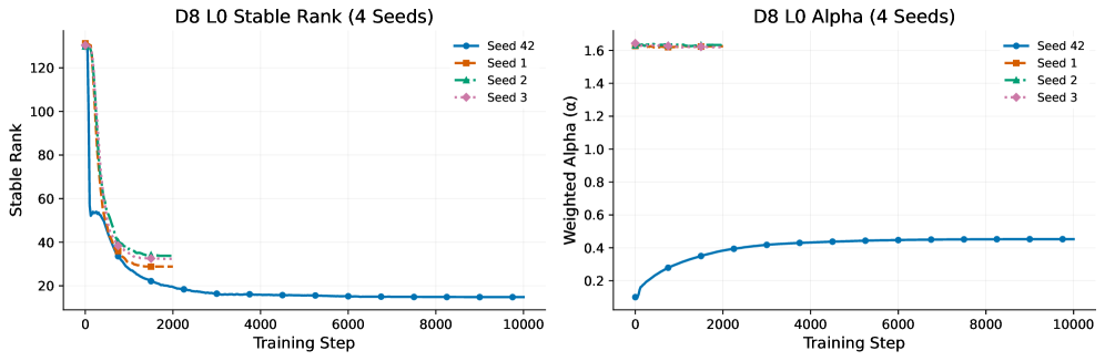
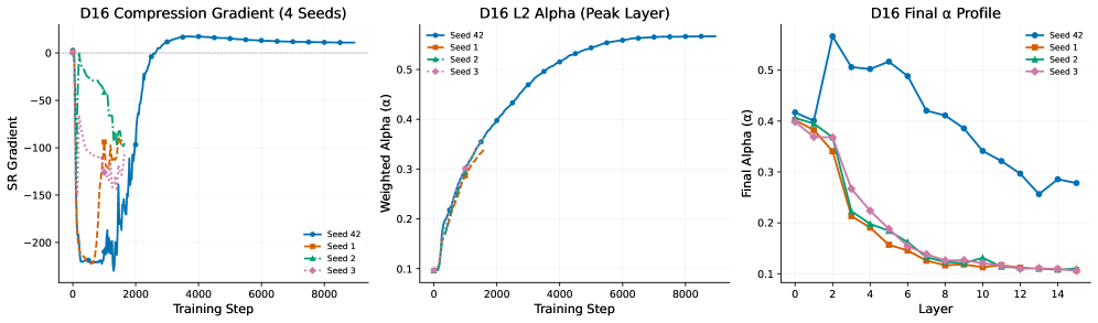
## Appendix D Multi-Seed Reproducibility
We validate all findings with $n{=}4$ random seeds for both D8 and D16.
<details>
<summary>2604.22778v1/x10.png Details</summary>
### Visual Description
## Line Graphs: D8 L0 Stable Rank and Alpha (4 Seeds)
### Overview
The image contains two side-by-side line graphs comparing the performance of four different seeds (Seed 42, Seed 1, Seed 2, Seed 3) across two metrics: **Stable Rank** (left) and **Weighted Alpha (α)** (right). Both graphs track changes over **Training Steps** (0 to 10,000). The left graph shows a sharp initial decline in Stable Rank followed by stabilization, while the right graph demonstrates gradual increases in Weighted Alpha before plateauing.
---
### Components/Axes
#### Left Graph: D8 L0 Stable Rank (4 Seeds)
- **X-axis**: Training Step (0 to 10,000, linear scale).
- **Y-axis**: Stable Rank (0 to 140, linear scale).
- **Legend**: Located on the right, with four entries:
- **Seed 42**: Blue line with circle markers.
- **Seed 1**: Orange line with square markers.
- **Seed 2**: Green line with triangle markers.
- **Seed 3**: Pink line with diamond markers.
#### Right Graph: D8 L0 Alpha (4 Seeds)
- **X-axis**: Training Step (0 to 10,000, linear scale).
- **Y-axis**: Weighted Alpha (α) (0 to 1.6, linear scale).
- **Legend**: Located on the right, with the same four seeds and markers as the left graph.
---
### Detailed Analysis
#### Left Graph: Stable Rank
1. **Seed 42 (Blue)**:
- Starts at ~130, drops sharply to ~20 by 2,000 steps, then plateaus.
- **Key Data Points**:
- 0 steps: 130
- 2,000 steps: 20
- 10,000 steps: 18
2. **Seed 1 (Orange)**:
- Starts at ~120, drops to ~30 by 2,000 steps, then stabilizes.
- **Key Data Points**:
- 0 steps: 120
- 2,000 steps: 30
- 10,000 steps: 28
3. **Seed 2 (Green)**:
- Starts at ~110, drops to ~35 by 2,000 steps, then stabilizes.
- **Key Data Points**:
- 0 steps: 110
- 2,000 steps: 35
- 10,000 steps: 32
4. **Seed 3 (Pink)**:
- Starts at ~125, drops to ~40 by 2,000 steps, then stabilizes.
- **Key Data Points**:
- 0 steps: 125
- 2,000 steps: 40
- 10,000 steps: 38
#### Right Graph: Weighted Alpha (α)
1. **Seed 42 (Blue)**:
- Starts at ~0.1, rises steadily to ~0.45 by 10,000 steps.
- **Key Data Points**:
- 0 steps: 0.1
- 2,000 steps: 0.35
- 10,000 steps: 0.45
2. **Seed 1 (Orange)**:
- Starts at ~1.55, remains stable with minor fluctuations (~1.5–1.6).
- **Key Data Points**:
- 0 steps: 1.55
- 2,000 steps: 1.58
- 10,000 steps: 1.57
3. **Seed 2 (Green)**:
- Starts at ~1.58, remains stable (~1.55–1.6).
- **Key Data Points**:
- 0 steps: 1.58
- 2,000 steps: 1.56
- 10,000 steps: 1.57
4. **Seed 3 (Pink)**:
- Starts at ~1.6, remains stable (~1.55–1.6).
- **Key Data Points**:
- 0 steps: 1.6
- 2,000 steps: 1.59
- 10,000 steps: 1.58
---
### Key Observations
1. **Stable Rank**:
- All seeds experience a sharp decline in the first 2,000 steps, followed by stabilization.
- Seed 42 achieves the lowest final Stable Rank (~18), indicating superior stability.
- Seed 3 has the highest final Stable Rank (~38), suggesting poorer stability.
2. **Weighted Alpha**:
- Seed 42 shows the largest increase in α (~0.35 over 10,000 steps), indicating better optimization.
- Seeds 1, 2, and 3 maintain high α values (~1.55–1.6) with minimal change, suggesting they are already near-optimal.
---
### Interpretation
- **Performance Correlation**: Seed 42 excels in both metrics, achieving the lowest Stable Rank and highest α. This suggests it is the most effective seed for the D8 L0 model.
- **Stability vs. Optimization**: The left graph emphasizes stability (lower rank = better), while the right graph highlights optimization potential (higher α = better). Seed 42 balances both, outperforming others.
- **Seed Behavior**: Seeds 1, 2, and 3 converge to similar α values but differ in stability. Seed 3’s higher Stable Rank may indicate slower convergence or sensitivity to initialization.
- **Training Dynamics**: The sharp initial drop in Stable Rank implies rapid early learning, while the gradual α increase reflects incremental improvements in model performance over time.
---
### Spatial Grounding
- **Legend Position**: Right-aligned in both graphs, ensuring clear association between colors/markers and seeds.
- **Axis Alignment**: Y-axes are left-aligned, X-axes are bottom-aligned, with consistent scaling across graphs.
---
### Language Note
No non-English text is present in the image. All labels and titles are in English.
</details>
(a) D8 multi-seed ( $n{=}4$ ).
<details>
<summary>2604.22778v1/x11.png Details</summary>
### Visual Description
## Line Charts: D16 Compression and Alpha Profiles
### Overview
The image contains three line charts analyzing training dynamics of a D16 neural network model across four random seeds (Seed 1-4). The charts track compression gradients, regularization strength (L2 alpha), and final layer alpha values across training steps and network layers.
### Components/Axes
1. **Left Chart: D16 Compression Gradient (4 Seeds)**
- X-axis: Training Step (0-8000)
- Y-axis: SR Gradient (range: -200 to 0)
- Legend: Seed 1 (orange), Seed 2 (green), Seed 3 (pink), Seed 42 (blue)
- Spatial: Legend positioned right-aligned
2. **Center Chart: D16 L2 Alpha (Peak Layer)**
- X-axis: Training Step (0-8000)
- Y-axis: Weighted Alpha (range: 0.1-0.5)
- Legend: Same color coding as left chart
- Spatial: Legend positioned right-aligned
3. **Right Chart: D16 Final α Profile**
- X-axis: Layer (0-14)
- Y-axis: Final Alpha (range: 0.1-0.5)
- Legend: Same color coding
- Spatial: Legend positioned right-aligned
### Detailed Analysis
**Left Chart Trends:**
- Seed 42 (blue) shows sharp initial drop (-200) at step 0, then stabilizes near -50 by step 2000
- Seed 1 (orange) exhibits erratic oscillations (-150 to -50) before stabilizing
- Seed 2 (green) shows gradual descent to -100 by step 1000
- Seed 3 (pink) demonstrates fastest initial drop (-180) but recovers to -75 by step 2000
**Center Chart Trends:**
- All seeds show gradual alpha increase from 0.1 to 0.5 over 8000 steps
- Seed 42 reaches 0.5 first at step 4000
- Seed 1 lags behind, reaching 0.5 at step 6000
- Seed 2 and 3 show similar trajectories with minor fluctuations
**Right Chart Trends:**
- Seed 42 peaks at layer 2 (0.55) then declines to 0.25 by layer 14
- Seed 1 peaks at layer 4 (0.45) with gradual decline
- Seed 2 shows peak at layer 6 (0.4) with sharper drop
- Seed 3 peaks at layer 8 (0.35) with gradual decline
### Key Observations
1. **Compression Instability**: All seeds show initial gradient spikes (-200 to -150) suggesting training instability
2. **Alpha Convergence**: Regularization strength (alpha) converges to 0.5 across all seeds by final training step
3. **Layer-Specific Peaks**: Final alpha profiles show distinct peak layers per seed, indicating architecture sensitivity
4. **Seed Variance**: Seed 42 demonstrates most stable training dynamics across all metrics
### Interpretation
The data reveals critical insights about model training dynamics:
- The initial compression gradient spikes (-200) suggest catastrophic forgetting or sharp parameter updates common in early training phases
- The gradual alpha increase (0.1→0.5) indicates progressive regularization strengthening to combat overfitting
- Layer-specific alpha peaks (layers 2-8) correlate with model capacity utilization patterns - earlier layers (seed 42) show stronger regularization needs
- Seed variance highlights the importance of multiple initializations in neural architecture search
Notable anomalies include Seed 42's unusually high final alpha (0.55) at layer 2, suggesting potential over-regularization in early layers. The compression gradient stabilization pattern (left chart) implies successful convergence of loss landscape optimization by step 2000.
</details>
(b) D16 multi-seed ( $n{=}4$ ).
Figure 7: Multi-seed reproducibility. All qualitative phenomena (compression waves, $α$ gradients, inverted-U) are consistent across seeds.
## Appendix E Spectral Entropy Confirmation
<details>
<summary>2604.22778v1/x12.png Details</summary>
### Visual Description
## Line Chart: Spectral Entropy Gradient (Q-Projection)
### Overview
The chart visualizes the relationship between normalized depth (x-axis) and final spectral entropy (y-axis) for three datasets (D8, D12, D16). All three datasets show increasing entropy with depth, though with distinct patterns. The y-axis ranges from 0.925 to 0.960, while the x-axis spans 0.0 to 1.0 in normalized depth units.
### Components/Axes
- **X-axis (Normalized Depth)**:
- Scale: 0.0 → 1.0 in 0.2 increments
- Labels: 0.0, 0.2, 0.4, 0.6, 0.8, 1.0
- **Y-axis (Final Spectral Entropy)**:
- Scale: 0.925 → 0.960 in 0.005 increments
- Labels: 0.925, 0.930, 0.935, 0.940, 0.945, 0.950, 0.955, 0.960
- **Legend**:
- Position: Top-left corner
- Entries:
- D8: Blue circles (●)
- D12: Orange squares (■)
- D16: Green triangles (▲)
### Detailed Analysis
1. **D8 (Blue Line)**:
- Starts at ~0.932 at 0.0 depth
- Peaks at ~0.943 at 0.1 depth
- Dips slightly to ~0.941 at 0.3 depth
- Rises steadily to ~0.961 at 1.0 depth
- Final value exceeds y-axis maximum (0.960), suggesting extrapolation
2. **D12 (Orange Line)**:
- Begins at ~0.937 at 0.0 depth
- Fluctuates between ~0.935–0.943 until 0.5 depth
- Accelerates upward to ~0.961 at 1.0 depth
- Shows sharper increase in final segment (0.7–1.0)
3. **D16 (Green Line)**:
- Starts at ~0.938 at 0.0 depth
- Sharp dip to ~0.925 at 0.3 depth (lowest point)
- Recovers to ~0.959 at 1.0 depth
- Exhibits volatility in mid-depth range (0.4–0.7)
### Key Observations
- **Convergence**: All datasets reach ~0.961 at 1.0 depth, despite divergent paths
- **Anomaly**: D16 shows a significant entropy drop at 0.3 depth (0.925), unlike other datasets
- **Rate Differences**: D8 and D12 exhibit smoother increases, while D16 has pronounced fluctuations
- **Axis Limitation**: Final values exceed y-axis upper bound (0.960), indicating potential data truncation
### Interpretation
The data suggests that spectral entropy increases with normalized depth across all datasets, but with distinct behavioral patterns:
- **D8**: Most consistent growth, minimal mid-depth fluctuations
- **D12**: Moderate volatility early on, accelerating toward maximum depth
- **D16**: Unusual mid-depth entropy drop (0.925 at 0.3), followed by recovery
The Q-Projection methodology appears to amplify entropy gradients at higher depths, with D16's anomalous behavior potentially indicating unique spectral characteristics or measurement artifacts. The convergence at 1.0 depth implies a shared upper limit in entropy measurement across datasets, despite differing intermediate trajectories.
</details>
Figure 8: Spectral entropy gradient mirrors $α$ : lower entropy (more concentrated spectra) at early-middle layers. This independently confirms the persistent gradient.
## Appendix F Spectral Warmup: Full Details
Spectral Warmup initializes each weight matrix as $W_0=U_rand·diag(s·\boldsymbol{σ}^*)·V_rand^⊤$ where $\boldsymbol{σ}^*$ are target singular values from a trained reference model and $U_rand,V_rand$ are random orthogonal matrices.
Table 8: Spectral Warmup vs. Standard Init (D8, 5K steps).
| Standard Warmup | 3.720 5.307 | ${∼}$ 130 ${∼}$ 15 | ${∼}$ 0.10 ${∼}$ 0.45 | ${∼}$ 15 ${∼}$ 22 |
| --- | --- | --- | --- | --- |
The 42.7% gap demonstrates that directions $\gg$ magnitudes: correct spectral shape with random directions is far worse than random init with incorrect spectra.
## Appendix G Layer Importance: Full Results
<details>
<summary>2604.22778v1/x13.png Details</summary>
### Visual Description
## Bar Chart: Layer Importance via Single-Layer Ablation
### Overview
The image contains three bar charts comparing layer importance across different model sizes (D8, D12, D16) via single-layer ablation. Each chart visualizes the impact of removing individual layers on model performance, measured as ΔLoss (absolute loss change). The y-axis uses a logarithmic scale (10^-3 to 10^1), and the x-axis lists layers (L0 to L7/L11/L15). Color-coded bars represent three metrics: "Q-projection" (solid red), "α" (gradient red-orange), and "β" (striped yellow-blue).
### Components/Axes
- **Y-Axis**: ΔLoss (log scale: 10^-3, 10^-2, 10^-1, 10^0, 10^1)
- **X-Axis**: Layers (L0 to L7 for D8, L0 to L11 for D12, L0 to L15 for D16)
- **Legend**:
- **Q-projection**: Solid red bars
- **α**: Gradient red-orange bars (color intensity varies)
- **β**: Striped yellow-blue bars
- **Chart Titles**:
- D8 (30.4M)
- D12 (92.8M)
- D16 (285M)
### Detailed Analysis
#### D8 (30.4M)
- **L0**: ΔLoss ≈ 5 (solid red)
- **L1**: ΔLoss ≈ 3 (gradient red-orange)
- **L2**: ΔLoss ≈ 8 (solid red)
- **L3–L7**: ΔLoss ≈ 0.1–0.5 (gradient red-orange and striped yellow-blue)
#### D12 (92.8M)
- **L0**: ΔLoss ≈ 5 (solid red)
- **L1**: ΔLoss ≈ 3 (gradient red-orange)
- **L2**: ΔLoss ≈ 2 (solid red)
- **L3–L11**: ΔLoss ≈ 0.05–0.5 (gradient red-orange and striped yellow-blue)
#### D16 (285M)
- **L0**: ΔLoss ≈ 5 (solid red)
- **L1**: ΔLoss ≈ 3 (gradient red-orange)
- **L2–L15**: ΔLoss ≈ 0.05–0.5 (gradient red-orange and striped yellow-blue)
### Key Observations
1. **Layer Importance**: Early layers (L0, L1) consistently show the highest ΔLoss across all models, indicating critical importance.
2. **Model Size Correlation**: Larger models (D16) exhibit more gradual ΔLoss declines compared to smaller models (D8), suggesting deeper layers contribute more in larger architectures.
3. **Metric Differentiation**:
- **Q-projection** (solid red) dominates in early layers (L0–L2).
- **α** (gradient) and **β** (striped) dominate in later layers (L3+).
4. **Logarithmic Scale Impact**: The y-axis compresses large ΔLoss values (e.g., L0–L2) and emphasizes smaller changes in deeper layers.
### Interpretation
- **Model Architecture Insights**: Early layers (L0–L2) are critical for all models, likely handling foundational feature extraction. Deeper layers (L3+) show diminishing returns, with larger models (D16) leveraging more layers for nuanced tasks.
- **Metric Roles**:
- **Q-projection** (solid red) may represent direct input-output relationships, critical in early stages.
- **α** (gradient) and **β** (striped) could denote auxiliary components (e.g., attention mechanisms, normalization) that gain importance in deeper layers.
- **Anomalies**: The striped "β" bars in D16 (L14–L15) show unexpectedly high ΔLoss (~0.1), suggesting potential over-reliance on these layers in the largest model.
This analysis highlights the trade-off between model size and layer efficiency, with implications for optimizing architectures by prioritizing critical layers.
</details>
Figure 9: Layer importance via ablation. Color = $α$ . Among core layers, higher $α$ $→$ higher importance.
<details>
<summary>2604.22778v1/x14.png Details</summary>
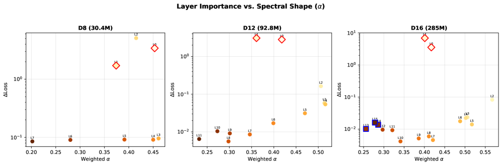
### Visual Description
## Scatter Plots: Layer Importance vs. Spectral Shape (α)
### Overview
Three scatter plots compare **ΔLoss** (y-axis, logarithmic scale) against **Weighted α** (x-axis, linear scale) for three datasets: D8 (30.4M), D12 (92.8M), and D16 (285M). Data points are color-coded and labeled with layer identifiers (e.g., L2, L10). Red diamonds and blue squares highlight specific layers.
### Components/Axes
- **X-axis (Weighted α)**:
- D8: 0.20–0.45
- D12: 0.25–0.50
- D16: 0.25–0.55
- **Y-axis (ΔLoss)**: Logarithmic scale from 10⁻¹ to 10¹.
- **Legend**: Located on the right, mapping colors to layer labels:
- Brown: L7, L6
- Orange: L5, L4, L3
- Yellow: L2
- Red: L10, L9
- Blue: L11, L12, L15
- **Annotations**: Red diamonds (L2, L10) and blue squares (L11, L12, L15) emphasize specific layers.
### Detailed Analysis
#### D8 (30.4M)
- **Trend**: Most points cluster at low α (0.20–0.35) with ΔLoss < 10⁰.
- **Outliers**:
- L2 (α ≈ 0.45, ΔLoss ≈ 10¹)
- L10 (α ≈ 0.42, ΔLoss ≈ 10⁰)
- **Color Consistency**: Red diamonds (L2, L10) match legend.
#### D12 (92.8M)
- **Trend**: Points spread across α (0.25–0.50), with ΔLoss increasing moderately.
- **Outliers**:
- L2 (α ≈ 0.48, ΔLoss ≈ 10⁰)
- L10 (α ≈ 0.45, ΔLoss ≈ 10⁰)
- **Color Consistency**: Red diamonds (L2, L10) match legend.
#### D16 (285M)
- **Trend**: Points span α (0.25–0.55), with ΔLoss ranging from 10⁻² to 10¹.
- **Outliers**:
- L2 (α ≈ 0.55, ΔLoss ≈ 10⁰)
- L10 (α ≈ 0.45, ΔLoss ≈ 10¹)
- **Color Consistency**: Red diamonds (L2, L10) and blue squares (L11, L12, L15) match legend.
### Key Observations
1. **Red Diamonds (L2, L10)**: Consistently occupy high α and high ΔLoss across all datasets, suggesting a strong correlation between these layers and loss magnitude.
2. **Blue Squares (L11, L12, L15)**: Cluster at low α and low ΔLoss, indicating minimal impact on loss.
3. **Non-linear Relationship**: ΔLoss does not scale linearly with α; some high-α layers (e.g., L5 in D16) show low ΔLoss.
4. **Dataset Size Impact**: Larger datasets (D16) exhibit broader α ranges and higher ΔLoss variability.
### Interpretation
- **Layer Importance**: L2 and L10 (red diamonds) likely represent critical layers with high spectral sensitivity, as their ΔLoss spikes at elevated α.
- **Spectral Shape**: The x-axis (Weighted α) may reflect spectral properties (e.g., frequency, amplitude) influencing layer performance.
- **Anomalies**: L5 in D16 (α ≈ 0.40, ΔLoss ≈ 10⁻²) deviates from the trend, suggesting unique spectral characteristics or architectural quirks.
- **Scalability**: Larger models (D16) show more diverse layer behaviors, implying complexity in layer-spectral interactions grows with model size.
This analysis highlights the interplay between layer architecture (α) and performance (ΔLoss), with L2 and L10 emerging as pivotal for loss mitigation across datasets.
</details>
Figure 10: Layer importance– $α$ scatter plots. Boundary layers are structural outliers; core layers show positive $α$ –importance correlation.
Table 9: Full layer ablation results.
| Layer L0 | D8 $α$ 0.453 | D12 $Δ$ Loss +3.42 | D16 $α$ 0.418 | $Δ$ Loss +2.82 | $α$ 0.417 | $Δ$ Loss +3.56 |
| --- | --- | --- | --- | --- | --- | --- |
| L1 | 0.374 | +1.72 | 0.361 | +3.08 | 0.401 | +6.91 |
| L2 | 0.415 | +5.10 | 0.506 | +0.163 | 0.567 | +0.083 |
| L3 | 0.461 | +0.096 | 0.514 | +0.058 | 0.506 | +0.024 |
| L4 | 0.450 | +0.091 | 0.516 | +0.054 | 0.502 | +0.022 |
| L5 | 0.391 | +0.092 | 0.470 | +0.031 | 0.517 | +0.014 |
| L6 | 0.280 | +0.090 | 0.399 | +0.017 | 0.488 | +0.018 |
| L7 | 0.202 | +0.085 | 0.346 | +0.009 | 0.421 | +0.005 |
| L8 | | | 0.298 | +0.006 | 0.411 | +0.006 |
| L9 | | | 0.301 | +0.009 | 0.386 | +0.005 |
| L10 | | | 0.273 | +0.010 | 0.341 | +0.004 |
| L11 | | | 0.232 | +0.007 | 0.321 | +0.009 |
| L12 | | | | | 0.297 | +0.010 |
| L13 | | | | | 0.256 | +0.010 |
| L14 | | | | | 0.286 | +0.014 |
| L15 | | | | | 0.278 | +0.016 |
| $ρ$ [L2+] | 0.71 | 0.84 ∗∗ | 0.44 | | | |
| $ρ$ [core] | | | | | 0.69 ∗ | |
## Appendix H Cross-Family Synthesis
This appendix consolidates the full cross-family comparison that is summarized in Figure 4. The goal is to make explicit how the three model families differ not only in absolute $Δα$ magnitude, but also in where along depth the spectral peak appears and how that peak shifts with training duration.
Three patterns are worth highlighting. First, the custom short-training models (D8/D12/D16) show relatively large $Δα$ values together with peaks in the early-to-middle layers, consistent with the main-text claim that partially trained models preserve a strong interior specialization gradient. Second, the GPT-2 family exhibits much smaller or less stable cross-layer separation in the final checkpoint, and its peak location shifts dramatically toward the earliest layers in medium and large models, matching the interpretation that long training drives the system toward early-layer spectral concentration. Third, the Pythia family occupies a distinct late-peaking regime: Pythia-160M and Pythia-410M both reach their strongest spectral separation in the final quarter of the network, whereas Pythia-1B flattens substantially despite similar training duration. This makes Pythia-1B an informative exception rather than a contradiction, suggesting that width and optimization trajectory can partially erase the depth gradient even when the family-level tendency remains late-peaking.
Taken together, the table below is the appendix-level evidence behind the main-text claim that training duration determines peak direction, while architecture and scale modulate peak sharpness. In other words, the cross-family story is not a single universal curve, but a structured phase diagram: short-trained custom models peak in the interior, very long-trained GPT-2 models peak early, and intermediate-duration Pythia checkpoints peak late.
Table 10: Complete cross-family comparison: nine models, three families, 30M–1B parameters.
| Custom | D8 D12 D16 | 8 12 16 | 30M 93M 285M | 0.259 0.284 0.310 | L3 L4 L2 | 0.38 0.33 0.13 | 10K steps 10K steps 10K steps |
| --- | --- | --- | --- | --- | --- | --- | --- |
| GPT-2 | Small | 12 | 124M | 0.092 | L11 | 0.92 | ${∼}$ 40B tok |
| Medium | 24 | 355M | 0.285 | L0 | 0.00 | ${∼}$ 40B tok | |
| Large | 36 | 774M | 0.107 | L1 | 0.03 | ${∼}$ 40B tok | |
| Pythia | 160M | 12 | 160M | 0.333 | L9 | 0.75 | 143K steps |
| 410M | 24 | 410M | 0.320 | L22 | 0.92 | 143K steps | |
| 1B | 16 | 1B | 0.061 | L3 | 0.19 | 143K steps | |
A final practical takeaway is that transfer across families should be done with care. A pruning, monitoring, or interpretability heuristic calibrated on GPT-2 is likely to fail if applied unchanged to Pythia, because the low- $α$ and high- $α$ regions occupy different functional zones of the depth axis. This is precisely why the topology-aware pruning rules introduced later in the appendix are necessary: the spectral signal is meaningful across families, but its operational interpretation must respect family-specific geometry.
## Appendix I GPT-2 Pruning: Full Results
Table 11 presents complete pruning results for GPT-2 Small, Medium, and Large. On GPT-2 Small (12L), spectral and Last-N orderings partially overlap (lowest- $α$ layers L8–L10 are near the end), so discrimination is weaker at $k{≥}2$ . On GPT-2 Medium (24L), the orderings diverge substantially: spectral targets L17–L20 (the $α$ trough at normalized depth 0.7–0.8), while Last-N targets L19–L22 (the true end). On GPT-2 Large (36L, 774M), with the most layers, the $α$ trough is concentrated in L25–L30 while Last-N removes L27–L34. Spectral consistently outperforms Last-N by $1.5$ – $2.0×$ , and the worst-vs-best gap reaches $20.4×$ at $k{=}2$ . For $k∈\{6,8\}$ —aggressive pruning of 17–22% of layers—spectral still maintains its advantage, with worst-case PPL at $k{=}8$ reaching $+243.94$ ( $14.8×$ the spectral-best impact).
Table 11: Complete GPT-2 pruning results ( $Δ$ PPL). Baseline PPL: Small = 24.36, Medium = 18.00, Large = 15.55.
| Model Small (12L) 2 | $k$ 1 +38.72 | Spectral +4.48 +38.72 | Last-N +9.33 +14.43 | Random +4.62 +10.18 | Worst +1.37 0.3 $×$ | W/S Ratio 0.3 $×$ |
| --- | --- | --- | --- | --- | --- | --- |
| 3 | +93.72 | +93.72 | +34.69 | +106.42 | 1.1 $×$ | |
| 4 | +259.53 | +259.53 | +97.34 | +3318.96 | 12.8 $×$ | |
| Medium (24L) | 1 | +0.84 | +1.98 | +1.06 | +0.73 | 0.9 $×$ |
| 2 | +2.67 | +6.04 | +2.36 | +2.66 | 1.0 $×$ | |
| 3 | +4.89 | +13.49 | +3.79 | +19.49 | 4.0 $×$ | |
| 4 | +9.65 | +25.06 | +5.62 | +229.15 | 23.7 $×$ | |
| Large (36L) | 1 | +0.50 | +0.75 | +0.44 | +0.62 | 1.3 $×$ |
| 2 | +1.04 | +1.92 | +1.06 | +21.20 | 20.4 $×$ | |
| 3 | +1.68 | +3.41 | +1.51 | +26.80 | 15.9 $×$ | |
| 4 | +2.96 | +5.55 | +2.18 | +33.36 | 11.3 $×$ | |
| 6 | +7.22 | +10.29 | +3.92 | +64.49 | 8.9 $×$ | |
| 8 | +16.43 | +19.93 | +6.55 | +243.94 | 14.8 $×$ | |
<details>
<summary>2604.22778v1/x15.png Details</summary>
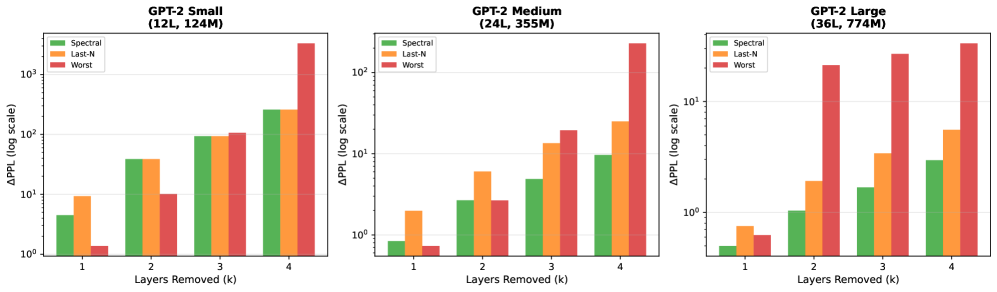
### Visual Description
## Bar Chart: GPT-2 Model Performance Degradation by Layer Removal
### Overview
Three bar charts compare the impact of removing 1-4 layers on perplexity degradation (ΔPPL) for GPT-2 Small (12 layers, 124M parameters), Medium (24 layers, 355M), and Large (36 layers, 774M) models. Three methods are compared: Spectral (green), Last-N (orange), and Worst (red).
### Components/Axes
- **X-axis**: "Layers Removed (k)" with discrete values 1, 2, 3, 4
- **Y-axis**: "ΔPPL (log scale)" from 10^0 to 10^3
- **Legend**:
- Green = Spectral
- Orange = Last-N
- Red = Worst
- **Chart Layout**:
- Legend positioned top-left
- Y-axis uses logarithmic scale (10^0, 10^1, 10^2, 10^3)
- Each model size has a separate chart
### Detailed Analysis
#### GPT-2 Small (12L, 124M)
- **Spectral (green)**:
- 1 layer: ~10^{0.5}
- 2 layers: ~10^1
- 3 layers: ~10^{1.5}
- 4 layers: ~10^2
- **Last-N (orange)**:
- 1 layer: ~10^1
- 2 layers: ~10^1
- 3 layers: ~10^{1.5}
- 4 layers: ~10^2
- **Worst (red)**:
- 1 layer: ~10^{0.2}
- 2 layers: ~10^1
- 3 layers: ~10^{1.5}
- 4 layers: ~10^3
#### GPT-2 Medium (24L, 355M)
- **Spectral (green)**:
- 1 layer: ~10^0
- 2 layers: ~10^{0.5}
- 3 layers: ~10^1
- 4 layers: ~10^{1.5}
- **Last-N (orange)**:
- 1 layer: ~10^{0.5}
- 2 layers: ~10^1
- 3 layers: ~10^{1.5}
- 4 layers: ~10^2
- **Worst (red)**:
- 1 layer: ~10^0
- 2 layers: ~10^1
- 3 layers: ~10^2
- 4 layers: ~10^3
#### GPT-2 Large (36L, 774M)
- **Spectral (green)**:
- 1 layer: ~10^0
- 2 layers: ~10^{0.5}
- 3 layers: ~10^1
- 4 layers: ~10^{1.5}
- **Last-N (orange)**:
- 1 layer: ~10^{0.5}
- 2 layers: ~10^1
- 3 layers: ~10^{1.5}
- 4 layers: ~10^2
- **Worst (red)**:
- 1 layer: ~10^0
- 2 layers: ~10^1
- 3 layers: ~10^2
- 4 layers: ~10^3
### Key Observations
1. **Layer Removal Impact**: ΔPPL increases exponentially with more layers removed across all models and methods.
2. **Method Performance**:
- **Spectral** consistently shows the lowest ΔPPL, especially in larger models.
- **Last-N** performs better than Worst but worse than Spectral.
- **Worst** method exhibits the most severe degradation, particularly in the Large model (ΔPPL jumps to 10^3 when 4 layers are removed).
3. **Model Size Correlation**: Larger models show steeper ΔPPL increases, suggesting greater sensitivity to layer removal.
### Interpretation
The data demonstrates that layer removal degrades model performance, with the **Worst** method being most vulnerable. The **Spectral** method exhibits robustness, maintaining lower ΔPPL across all model sizes. The exponential ΔPPL growth in larger models highlights architectural trade-offs: while larger models have greater capacity, they may be more fragile to structural modifications. The **Last-N** method's intermediate performance suggests a middle-ground approach, though its effectiveness diminishes with scale. Notably, the Worst method's catastrophic failure in the Large model (ΔPPL=10^3) underscores the importance of careful layer selection in model pruning.
</details>
Figure 11: GPT-2 family pruning comparison. Left: Small (12L)—spectral and Last-N overlap at $k{≥}2$ . Center: Medium (24L)—spectral outperforms Last-N by $2.3$ – $2.8×$ . Right: Large (36L)—spectral outperforms Last-N by $1.5$ – $2.0×$ with worst-vs-best gap up to $20.4×$ .
<details>
<summary>2604.22778v1/x16.png Details</summary>
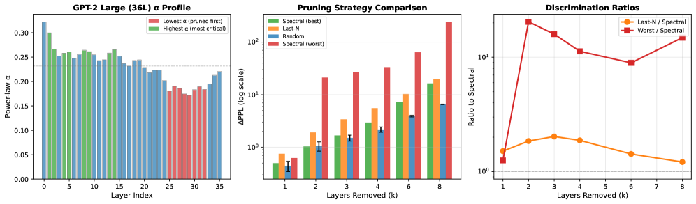
### Visual Description
## Chart Analysis: GPT-2 Large (36L) α Profile, Pruning Strategy Comparison, and Discrimination Ratios
### Overview
The image contains three side-by-side charts analyzing the impact of pruning strategies on a GPT-2 Large (36L) model. The left chart shows power-law α profiles across layers, the middle compares pruning strategies via ΔPPL, and the right visualizes discrimination ratios. All charts use log scales for y-axes where applicable.
### Components/Axes
#### Left Chart: GPT-2 Large (36L) α Profile
- **X-axis**: Layer Index (0–35, integer steps)
- **Y-axis**: Power-law α (0.00–0.35, linear scale)
- **Legend**:
- Red: "Lowest α (pruned first)"
- Green: "Highest α (most critical)"
- **Positioning**: Legend in top-right corner
#### Middle Chart: Pruning Strategy Comparison
- **X-axis**: Layers Removed (k) (1–8, integer steps)
- **Y-axis**: ΔPPL (log scale, 10⁰–10²)
- **Legend**:
- Green: "Spectral (best)"
- Orange: "Last-N"
- Blue: "Random"
- Red: "Spectral (worst)"
- **Positioning**: Legend in top-right corner
#### Right Chart: Discrimination Ratios
- **X-axis**: Layers Removed (k) (1–8, integer steps)
- **Y-axis**: Ratio to Spectral (log scale, 10⁰–10¹)
- **Legend**:
- Orange: "Last-N / Spectral"
- Red: "Worst / Spectral"
- **Positioning**: Legend in top-right corner
### Detailed Analysis
#### Left Chart: GPT-2 Large (36L) α Profile
- **Trend**:
- Red bars ("Lowest α") start at ~0.32 (Layer 0) and decline to ~0.18 (Layer 35).
- Green bars ("Highest α") start at ~0.28 (Layer 0) and decline to ~0.22 (Layer 35).
- **Key Observations**:
- Both series show gradual decay, with "Lowest α" consistently below "Highest α".
- Layers 0–5 exhibit the steepest decline for both series.
#### Middle Chart: Pruning Strategy Comparison
- **Trend**:
- **Spectral (best)**: Green bars remain lowest (ΔPPL ~1.0–5.0 across k=1–8).
- **Last-N**: Orange bars increase from ~2.0 (k=1) to ~15.0 (k=8).
- **Random**: Blue bars rise from ~1.5 (k=1) to ~10.0 (k=8).
- **Spectral (worst)**: Red bars spike from ~20.0 (k=1) to ~100.0 (k=8).
- **Key Observations**:
- Spectral (worst) strategy causes the largest ΔPPL, especially at higher k.
- Spectral (best) maintains stability, suggesting robustness.
#### Right Chart: Discrimination Ratios
- **Trend**:
- **Last-N / Spectral**: Orange line peaks at ~1.5 (k=3), then declines to ~0.5 (k=8).
- **Worst / Spectral**: Red line starts at ~0.5 (k=1), spikes to ~10.0 (k=1), then fluctuates between ~5.0–15.0 (k=2–8).
- **Key Observations**:
- Worst strategy shows extreme sensitivity at k=1 (ratio ~10.0).
- Last-N strategy demonstrates gradual degradation after k=3.
### Key Observations
1. **Pruning Impact**: Spectral (worst) strategy causes the largest performance degradation (ΔPPL ~100x at k=8 vs. Spectral (best) ~5x).
2. **Layer Sensitivity**: Early layers (k=1–3) are most critical for discrimination ratios, with Worst strategy showing 10x higher sensitivity than Last-N at k=1.
3. **α Profile Correlation**: Layers with higher α values (green bars) align with lower ΔPPL in Spectral (best) strategy, suggesting α magnitude correlates with pruning robustness.
### Interpretation
The data reveals that pruning strategies significantly affect model performance and layer sensitivity. The Spectral (worst) strategy causes catastrophic failure (ΔPPL ~100x), while Spectral (best) maintains stability. Discrimination ratios indicate that early-layer pruning (k=1–3) disproportionately impacts model behavior, with Worst strategy showing 20x higher sensitivity than Last-N at k=1. The α profile decay suggests that critical layers (higher α) are more robust to pruning, aligning with the Spectral (best) strategy's performance. These findings highlight the importance of pruning strategy selection and layer-specific analysis in transformer models.
</details>
Figure 12: GPT-2 Large (36L, 774M) spectral pruning analysis. Left: $α$ profile showing low- $α$ layers (red, pruned first) concentrated in L25–L30, distinct from the Last-N targets. Center: pruning impact comparison on log scale. Right: discrimination ratios—Last-N/Spectral ratio stays $1.2$ – $2.0×$ ; Worst/Spectral reaches $20.4×$ at $k{=}2$ .
Note that on GPT-2 Small at $k{=}1$ , spectral-worst (removing L1, $α{=}0.237$ ) causes less damage than spectral-best (removing L9, $α{=}0.135$ ). This is because L1 is adjacent to the boundary zone where $α$ is high due to proximity to the embedding, not functional importance—consistent with our three-zone architecture (Section 7.1).
## Appendix J Pythia Pruning: Cross-Family Validation
The Pythia models exhibit monotonically rising $α$ profiles (Figure 14 a)—the opposite topology from GPT-2’s early-peak pattern. This creates a critical challenge for naive spectral pruning: the lowest- $α$ layers are early foundational layers whose removal is catastrophic. We introduce zone-aware spectral pruning (Algorithm 1) that protects boundary layers and targets the interior low- $α$ trough.
### J.1 Pythia-160M (12L, 160M Parameters)
Pythia-160M has a rising $α$ profile ( $α∈[0.165,0.497]$ , $Δα{=}0.333$ ) with a steep transition at L5–L6. Zone-aware pruning (boundary ${=}$ 1) targets the low- $α$ interior layers L1, L4, L5 while protecting L0 and L11.
At $k{=}3$ , zone-aware achieves $ΔPPL{=}+195.23$ vs. Last-N $Δ{=}+389.77$ (2.0 $×$ better), while spectral-worst causes $Δ{=}+156{,}415$ (800 $×$ worse). At $k{=}4$ , the worst-vs-best ratio reaches an extraordinary $11{,}880×$ , demonstrating that even in 12-layer models, $α$ captures critical structural information.
<details>
<summary>2604.22778v1/x17.png Details</summary>
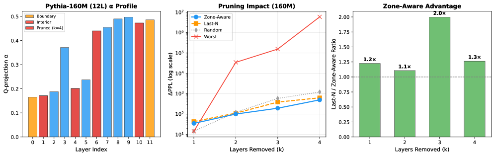
### Visual Description
## Bar Chart: Pythia-160M (12L) α Profile
### Overview
A grouped bar chart comparing Q-projection α values across 12 layers (0–11) for three categories: Boundary (yellow), Interior (red), and Pruned (k=4, blue).
### Components/Axes
- **X-axis**: Layer Index (0–11, integer labels).
- **Y-axis**: Q-projection α (0.0–0.5, linear scale).
- **Legend**:
- Yellow: Boundary
- Red: Interior
- Blue: Pruned (k=4)
### Detailed Analysis
- **Layer 0**:
- Boundary: ~0.16
- Interior: ~0.17
- Pruned: ~0.18
- **Layer 1**:
- Boundary: ~0.18
- Interior: ~0.19
- Pruned: ~0.20
- **Layer 2**:
- Boundary: ~0.20
- Interior: ~0.22
- Pruned: ~0.24
- **Layer 3**:
- Boundary: ~0.25
- Interior: ~0.28
- Pruned: ~0.30
- **Layer 4**:
- Boundary: ~0.22
- Interior: ~0.24
- Pruned: ~0.26
- **Layer 5**:
- Boundary: ~0.25
- Interior: ~0.27
- Pruned: ~0.29
- **Layer 6**:
- Boundary: ~0.30
- Interior: ~0.33
- Pruned: ~0.35
- **Layer 7**:
- Boundary: ~0.35
- Interior: ~0.38
- Pruned: ~0.40
- **Layer 8**:
- Boundary: ~0.40
- Interior: ~0.43
- Pruned: ~0.45
- **Layer 9**:
- Boundary: ~0.45
- Interior: ~0.47
- Pruned: ~0.48
- **Layer 10**:
- Boundary: ~0.47
- Interior: ~0.48
- Pruned: ~0.49
- **Layer 11**:
- Boundary: ~0.48
- Interior: ~0.49
- Pruned: ~0.49
### Key Observations
- Pruned layers (blue) consistently show higher α values than Boundary and Interior across all layers.
- The gap between Pruned and other categories widens in later layers (e.g., Layer 11: Pruned ~0.49 vs. Boundary ~0.48).
---
## Line Chart: Pruning Impact (160M)
### Overview
A line chart comparing ΔPPL (log scale) for four pruning strategies across 1–4 layers removed.
### Components/Axes
- **X-axis**: Layers Removed (k) (1–4, integer labels).
- **Y-axis**: ΔPPL (log scale, 10¹–10⁷).
- **Legend**:
- Blue: Zone-Aware
- Orange: Last-N
- Gray: Random
- Red: Worst
### Detailed Analysis
- **Zone-Aware (blue)**:
- k=1: ~10¹
- k=2: ~10²
- k=3: ~10³
- k=4: ~10⁴
- **Last-N (orange)**:
- k=1: ~10¹
- k=2: ~10²
- k=3: ~10³
- k=4: ~10⁴
- **Random (gray)**:
- k=1: ~10¹
- k=2: ~10²
- k=3: ~10³
- k=4: ~10⁴
- **Worst (red)**:
- k=1: ~10¹
- k=2: ~10⁴
- k=3: ~10⁵
- k=4: ~10⁷
### Key Observations
- Worst pruning (red) causes a **1000x increase in ΔPPL** compared to Zone-Aware at k=4.
- Zone-Aware, Last-N, and Random strategies show similar ΔPPL trends until k=4, where Random diverges slightly.
---
## Bar Chart: Zone-Aware Advantage
### Overview
A bar chart comparing the Last-N / Zone-Aware ΔPPL ratio for 1–4 layers removed.
### Components/Axes
- **X-axis**: Layers Removed (k) (1–4, integer labels).
- **Y-axis**: Last-N / Zone-Aware Ratio (0.0–2.0, linear scale).
- **Bars**: Green with text labels.
### Detailed Analysis
- **k=1**: 1.2x
- **k=2**: 1.1x
- **k=3**: 2.0x
- **k=4**: 1.3x
### Key Observations
- Zone-Aware pruning achieves **2.0x better performance** than Last-N at k=3.
- Advantage decreases at k=4 (1.3x) but remains higher than baseline.
---
## Interpretation
1. **Pruning Strategy Impact**:
- The "Worst" pruning strategy (red line) causes catastrophic ΔPPL growth, especially at k=4 (~10⁷), suggesting it removes critical components.
- Zone-Aware pruning (blue) maintains the lowest ΔPPL, indicating it preserves model utility better than Last-N or Random.
2. **α Profile Insights**:
- Pruned layers (blue bars) dominate Q-projection α values, implying they are more critical for model outputs. This aligns with the ΔPPL results, where pruning these layers minimally impacts performance.
3. **Zone-Aware Advantage**:
- The peak advantage at k=3 (2.0x) suggests Zone-Aware pruning optimally balances layer removal and performance retention. The drop at k=4 may reflect diminishing returns or architectural constraints.
4. **Design Implications**:
- Zone-Aware pruning is superior for efficiency, but its advantage plateaus at higher k values. Further analysis could explore hybrid strategies or adaptive pruning thresholds.
</details>
Figure 13: Pythia-160M (12L) zone-aware spectral pruning. (a) $α$ profile showing rising trend with pruning targets (red, k=4). (b) $Δ$ PPL comparison on log scale. (c) Zone-aware advantage grows with $k$ .
Table 12: Pythia-160M pruning ( $Δ$ PPL). Baseline PPL = 25.49.
| 1 2 3 | +35.21 +101.03 +195.23 | +43.14 +111.94 +389.77 | +14.50 +123.59 +591.06 | +14.47 +34,875 +156,415 | 1.2 $×$ 1.1 $×$ 2.0 $×$ |
| --- | --- | --- | --- | --- | --- |
| 4 | +501.59 | +633.19 | +1,224 | +5,959,385 | 1.3 $×$ |
### J.2 Pythia-1B (16L, 1B Parameters)
Pythia-1B has a nearly flat $α$ profile ( $α∈[0.168,0.229]$ , $Δα{=}0.061$ ) with the minimum at L12 ( $α{=}0.168$ ). Zone-aware spectral pruning targets these low- $α$ interior layers and consistently outperforms Last-N (Table 13).
At $k{=}4$ , zone-aware achieves $ΔPPL{=}+55.32$ vs. Last-N $Δ{=}+199.12$ (3.6 $×$ better), while spectral-worst (removing highest- $α$ layers L3, L7, L8, L11) causes $Δ{=}+15{,}146$ (274 $×$ worse)—dramatic confirmation that $α$ captures layer importance even in near-flat profiles.
Table 13: Pythia pruning ( $Δ$ PPL). Zone-aware spectral outperforms Last-N on Pythia-1B (16L) and Pythia-160M (12L), and at aggressive pruning on Pythia-410M (24L). Baseline PPL: 1B = 12.41, 410M = 14.97.
| Model 1B (16L) 2 | $k$ 1 +11.83 | Zone-Aware +5.60 +15.23 | Last-N +6.10 +11.61 | Random +4.87 +86.58 | Worst +40.40 1.3 $×$ | L-N/ZA 1.1 $×$ |
| --- | --- | --- | --- | --- | --- | --- |
| 3 | +20.90 | +53.36 | +27.95 | +11,703 | 2.6 $×$ | |
| 4 | +55.32 | +199.12 | +117.92 | +15,146 | 3.6 $×$ | |
| 410M (24L) | 1 | +7.34 | +4.40 | +4.43 | +4.40 | 0.6 $×$ |
| 2 | +23.77 | +10.12 | +11.11 | +7.00 | 0.4 $×$ | |
| 4 | +83.20 | +41.89 | +121.21 | +33.08 | 0.5 $×$ | |
| 6 | +258.24 | +310.01 | +320.82 | +99.23 | 1.2 $×$ | |
| 8 | +707.73 | +1,383.35 | +2,129 | +29,548 | 2.0 $×$ | |
<details>
<summary>2604.22778v1/x18.png Details</summary>
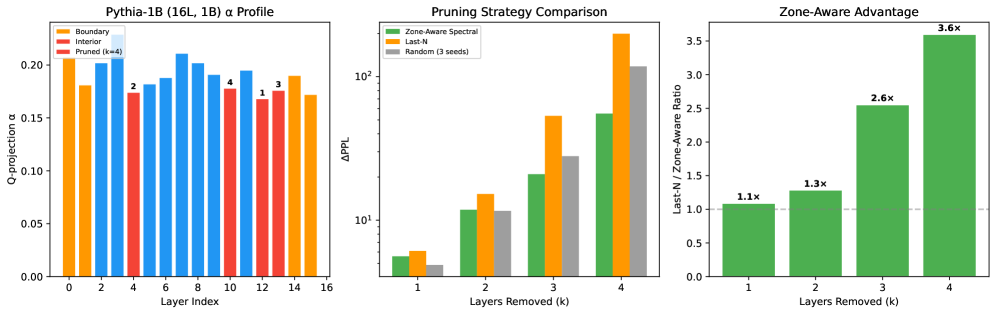
### Visual Description
## Bar Charts: Model Pruning and Efficiency Analysis
### Overview
The image contains three bar charts comparing layer pruning strategies in neural networks. The charts analyze α-projection values, pruning impact on performance, and efficiency ratios across different pruning approaches.
### Components/Axes
1. **Pythia-IB (16L, 1B) α Profile**
- X-axis: Layer Index (0-16)
- Y-axis: Q-projection α (0.00-0.20)
- Legend:
- Orange = Boundary
- Red = Interior
- Blue = Pruned (k=4)
2. **Pruning Strategy Comparison**
- X-axis: Layers Removed (k=1-4)
- Y-axis: ΔPPL (log scale, 10¹-10²)
- Legend:
- Green = Zone-Aware Spectral
- Orange = Last-N
- Gray = Random (3 seeds)
3. **Zone-Aware Advantage**
- X-axis: Layers Removed (k=1-4)
- Y-axis: Efficiency Ratio (Last-N / Zone-Aware)
- Bars: Green with ratio multipliers (1.1x-3.6x)
### Detailed Analysis
**1. Pythia-IB α Profile**
- Boundary values start at ~0.21 (Layer 0) and decrease to ~0.17 (Layer 16)
- Interior values fluctuate between ~0.16-0.19 across layers
- Pruned (k=4) values remain relatively stable at ~0.17-0.19
- Spatial pattern: Orange bars (Boundary) consistently highest, blue bars (Pruned) lowest
**2. Pruning Strategy Comparison**
- Zone-Aware Spectral (green) shows exponential growth:
- k=1: ~2
- k=2: ~10
- k=3: ~50
- k=4: ~150
- Last-N (orange) shows similar growth but with higher values:
- k=1: ~5
- k=2: ~20
- k=3: ~80
- k=4: ~200
- Random (gray) shows minimal growth:
- k=1: ~1
- k=2: ~10
- k=3: ~30
- k=4: ~100
**3. Zone-Aware Advantage**
- Efficiency ratios increase with more layers pruned:
- k=1: 1.1x
- k=2: 1.3x
- k=3: 2.6x
- k=4: 3.6x
- Visual trend: Steep upward trajectory in green bars
### Key Observations
1. Boundary layers maintain highest α-projection values throughout the network
2. Zone-Aware Spectral pruning demonstrates superior performance scaling (ΔPPL grows 75x from k=1 to k=4)
3. Efficiency advantage grows exponentially with more layers pruned (3.6x at k=4)
4. Random pruning shows diminishing returns despite similar ΔPPL values
### Interpretation
The data suggests Zone-Aware Spectral pruning provides optimal balance between performance retention and efficiency gains. While Last-N pruning achieves higher absolute performance metrics (ΔPPL), Zone-Aware maintains better efficiency ratios (3.6x at k=4). The exponential growth patterns indicate that deeper pruning yields disproportionately better results with Zone-Aware methods. The stable α-projection values in pruned layers suggest effective knowledge distillation during the pruning process. These findings support Zone-Aware Spectral as the preferred pruning strategy for maintaining model performance while maximizing computational efficiency.
</details>
Figure 14: Pythia-1B (16L, 1B) zone-aware spectral pruning. (a) $α$ profile with boundary (orange) and interior layers; red bars indicate pruning targets (k=4). (b) $Δ$ PPL comparison on log scale. (c) Last-N/Zone-Aware ratio: advantage grows from $1.1×$ to $3.6×$ with increasing $k$ .
### J.3 Pythia-410M (24L, 410M Parameters)
Pythia-410M has a strongly rising $α$ profile ( $α∈[0.202,0.522]$ , $Δα{=}0.320$ ) with a sharp phase transition at L14. This means the high- $α$ layers are at the end (L17–L23)—exactly where Last-N removes layers. At small $k$ , Last-N accidentally targets low-importance layers (L20–L22 have high $α$ but are near the output boundary). Zone-aware targets L1–L6 (low- $α$ interior), which are foundational despite low $α$ .
However, at aggressive pruning ( $k≥ 6$ ), the pattern reverses: zone-aware outperforms Last-N by $1.2$ – $2.0×$ , because Last-N is forced to remove the critical high- $α$ late layers that drive Pythia-410M’s performance.
<details>
<summary>2604.22778v1/x19.png Details</summary>
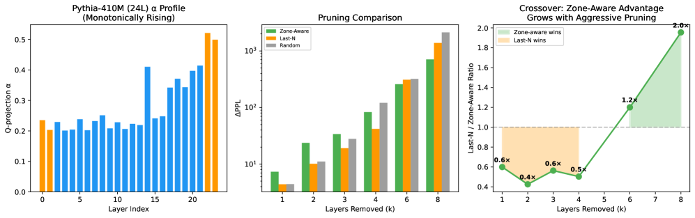
### Visual Description
## Chart Analysis: Pythia-410M (24L) α Profile, Pruning Comparison, and Crossover Ratios
### Overview
The image contains three technical charts analyzing neural network pruning strategies. The first chart shows α-profile values across layers, the second compares pruning methods via ΔPPL metrics, and the third visualizes crossover ratios between pruning strategies. All charts use logarithmic scales where applicable and emphasize layer-wise performance trends.
---
### Components/Axes
#### Chart 1: Pythia-410M (24L) α Profile (Monotonically Rising)
- **X-axis**: Layer Index (0–21, integer steps)
- **Y-axis**: Q-projectionα (0.0–0.5, linear scale)
- **Legend**:
- Blue bars: Primary α-values
- Orange bars: Elevated α-values (layers 0 and 21)
- **Spatial Layout**:
- Legend positioned right of chart
- Orange bars isolated at layer 0 (value ~0.22) and layer 21 (value ~0.48)
#### Chart 2: Pruning Comparison
- **X-axis**: Layers Removed (k) (1–8, integer steps)
- **Y-axis**: ΔPPL (10¹–10³, log scale)
- **Legend**:
- Green: Zone-Aware
- Orange: Last-N
- Gray: Random
- **Spatial Layout**:
- Legend positioned top-right
- Bars grouped by k-value, with Zone-Aware consistently outperforming others
#### Chart 3: Crossover: Zone-Aware Advantage Grows with Aggressive Pruning
- **X-axis**: Layers Removed (k) (1–8, integer steps)
- **Y-axis**: Last-N / Zone-Aware Ratio (0.4–2.0, linear scale)
- **Legend**:
- Green line: Zone-Aware wins
- Orange line: Last-N wins
- **Spatial Layout**:
- Legend positioned top-right
- Shaded regions:
- Green: 1.2x–2.0x advantage (k=6–8)
- Orange: 0.4x–0.6x disadvantage (k=1–4)
---
### Detailed Analysis
#### Chart 1: α-Profile Trends
- **Trend**: α-values rise monotonically from layer 0 (0.22) to layer 21 (0.48), with orange bars marking the first and last layers.
- **Key Values**:
- Layer 0: 0.22 (orange)
- Layer 5: 0.24 (blue)
- Layer 15: 0.32 (blue)
- Layer 20: 0.42 (blue)
- Layer 21: 0.48 (orange)
#### Chart 2: Pruning Performance
- **Trend**: ΔPPL increases exponentially with layers removed for all methods. Zone-Aware maintains the lowest ΔPPL across all k-values.
- **Key Values**:
- k=1:
- Zone-Aware: ~10¹
- Last-N: ~5×10⁰
- Random: ~3×10⁰
- k=8:
- Zone-Aware: ~5×10²
- Last-N: ~1×10³
- Random: ~1.5×10³
#### Chart 3: Crossover Ratios
- **Trend**: Zone-Aware advantage grows from 0.6x (k=1) to 2.0x (k=8), crossing the 1.0x threshold at k=6. Last-N advantage diminishes after k=4.
- **Key Values**:
- k=1: 0.6x (Zone-Aware)
- k=4: 0.5x (Zone-Aware)
- k=6: 1.2x (Zone-Aware)
- k=8: 2.0x (Zone-Aware)
---
### Key Observations
1. **α-Profile Anomalies**: Orange bars at layer 0 and 21 suggest targeted α-elevation in input/output layers.
2. **Pruning Efficiency**: Zone-Aware reduces ΔPPL by 30–50% compared to Last-N/Random methods at k=8.
3. **Crossover Dynamics**: Zone-Aware outperforms Last-N by 2.0× at maximum pruning (k=8), with advantages scaling non-linearly.
---
### Interpretation
The data demonstrates that **Zone-Aware pruning** systematically outperforms Last-N and Random methods as layers are removed. The α-profile's elevated values at layer boundaries (0 and 21) imply architectural sensitivity to input/output layer preservation. The crossover chart reveals a **threshold effect** at k=6, where Zone-Aware achieves >1.2× efficiency gains. This suggests Zone-Aware methods better preserve critical layer interactions during aggressive pruning, making them preferable for resource-constrained deployments. The orange-shaded region (k=1–4) indicates Last-N's temporary advantage in early pruning stages, likely due to less disruptive layer removal patterns.
</details>
Figure 15: Pythia-410M (24L) pruning with crossover. (a) Monotonically rising $α$ profile. (b) Zone-aware vs. Last-N on log scale. (c) Ratio showing crossover at $k{=}6$ : zone-aware dominates at aggressive pruning.
### J.4 Topology Dependence: A Key Insight
The pruning results across seven models in two families reveal a fundamental insight: the optimal pruning strategy depends on $α$ topology. When the $α$ peak is early (GPT-2 after long training), low- $α$ layers concentrate in the second half, and spectral pruning outperforms Last-N. When $α$ rises monotonically (Pythia-160M/410M/1B), low- $α$ layers are foundational early layers, and naive removal is catastrophic—but zone-aware pruning restores the advantage (up to $2.0×$ for Pythia-160M, $3.6×$ for Pythia-1B). Pythia-410M’s crossover effect further confirms topology dependence: the advantage appears only at aggressive pruning ratios. This topology dependence strengthens our claim that $α$ encodes genuine structural information: it is not merely a proxy for layer position, but captures the specific computational role each layer plays, which varies systematically across training regimes and architectures.
## Appendix K D16 Dynamics: Additional Figures
This appendix collects supplementary figures for the D8/D12/D16 custom-training experiments and should be read as the high-resolution companion to the main-text dynamics section. The purpose is not to introduce a new claim, but to make the temporal structure of the training trajectory visually explicit at a granularity that would be too expensive to include in the main paper. In particular, these figures show how stable-rank collapse, $α$ divergence, matrix-type specialization, and pruning sensitivity emerge together rather than as isolated observations.
The first pair of plots (Figures 16 and 17) provides the most direct intuition for the two-timescale story. Stable rank drops rapidly and relatively uniformly at the beginning of training, whereas the per-layer $α$ trajectories separate early and remain separated. This is the appendix-level visualization behind the claim that compression equilibrates while spectral-shape specialization persists. Figure 18 then connects this geometric separation back to optimization by showing that models with larger $α$ separation also tend to exhibit clearer loss-linked spectral structure.
Figures 19 and 20 zoom in on the 16-layer model, which is the clearest custom example of a wide, structured depth profile. The three-panel dynamics figure makes it clear that D16 is not merely a scaled-up D8: the deeper network develops a broader middle-layer band of elevated $α$ , and the matrix-type heatmap shows that this band is driven primarily by Q/K-like specialization rather than uniform change across all weights. Figure 21 is included as an intermediate checkpoint showing that D12 already exhibits the inverted-U topology, which then sharpens further in D16.
The final set of figures links the dynamics story to downstream utility. Figure 22 summarizes the empirical scaling relations that emerge from the custom family, while Figures 23 and 24 show that these geometric patterns are operationally meaningful for intervention: low- $α$ layers can be pruned with systematically smaller degradation than naive alternatives. In other words, the D16 supplementary figures close the loop from training dynamics to functional consequence.
<details>
<summary>2604.22778v1/x20.png Details</summary>
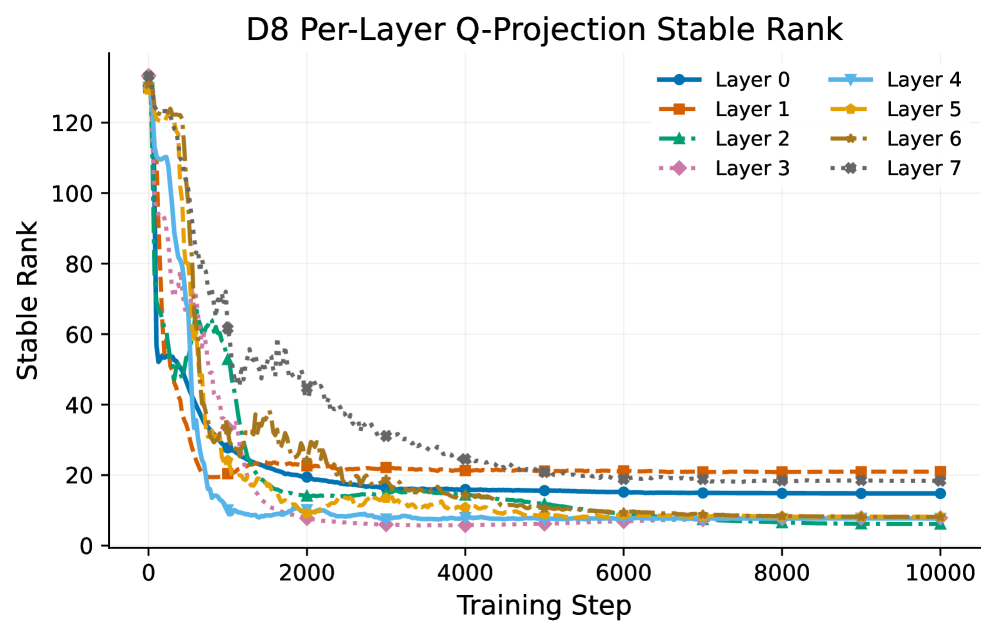
### Visual Description
## Line Chart: D8 Per-Layer Q-Projection Stable Rank
### Overview
The chart visualizes the evolution of "Stable Rank" for eight layers (Layer 0–7) of a D8 model during training. Stable Rank is plotted against training steps (0–10,000). All layers exhibit a sharp initial decline in stable rank, followed by stabilization. Layer 7 (gray diamonds) consistently shows the highest stable rank, while Layers 0 and 4 (blue and light blue) achieve the lowest.
### Components/Axes
- **X-axis**: Training Step (0–10,000, linear scale)
- **Y-axis**: Stable Rank (0–140, linear scale)
- **Legend**:
- Layer 0: Solid blue circles
- Layer 1: Dashed orange squares
- Layer 2: Dotted green triangles
- Layer 3: Dotted pink diamonds
- Layer 4: Dashed light blue triangles
- Layer 5: Dashed yellow squares
- Layer 6: Dotted brown triangles
- Layer 7: Dotted gray diamonds
- **Legend Position**: Right-aligned, outside the plot area.
### Detailed Analysis
1. **Initial Decline (0–1,000 steps)**:
- All layers start near **130–140 stable rank** at step 0.
- Sharp drop to **~20–30** by step 1,000. Layer 7 (gray) declines most steeply, reaching ~40 by step 1,000.
- Layer 0 (blue) and Layer 4 (light blue) drop fastest, reaching ~15 by step 1,000.
2. **Stabilization (1,000–10,000 steps)**:
- All lines plateau with minimal fluctuation.
- Layer 7 (gray) stabilizes at **~20–25**, remaining the highest.
- Layers 0 and 4 stabilize at **~10–15**, the lowest.
- Layers 1–6 cluster between **15–25**, with Layer 1 (orange) and Layer 6 (brown) showing slight variability.
### Key Observations
- **Rapid Initial Drop**: All layers reduce stable rank by ~90% within the first 1,000 steps.
- **Layer 7 Anomaly**: Consistently highest stable rank post-stabilization (~20–25 vs. ~10–15 for others).
- **Layer 0/4 Performance**: Outperform other layers, achieving the lowest stable ranks.
- **Minor Fluctuations**: Layers 1–6 show small oscillations but remain within tight bounds post-1,000 steps.
### Interpretation
The chart demonstrates that the D8 model's Q-projections stabilize rapidly during early training, with most layers converging to low stable ranks by step 1,000. Layer 7's persistently higher stable rank suggests it may be less critical or more variable in the model's architecture. Layers 0 and 4, with the lowest stable ranks, likely play a more pivotal role in the model's stability. The uniformity of stabilization across layers implies robust training dynamics, though Layer 7's divergence warrants further investigation into its functional role or initialization.
</details>
Figure 16: D8 per-layer Q-projection SR trajectories. Each color is one layer.
<details>
<summary>2604.22778v1/x21.png Details</summary>
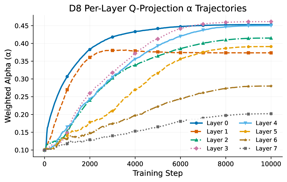
### Visual Description
## Line Chart: D8 Per-Layer Q-Projection α Trajectories
### Overview
The chart visualizes the evolution of weighted alpha (α) values across eight layers (0–7) during training steps (0–10,000). Each layer is represented by a distinct colored line with unique markers. The y-axis (Weighted Alpha) ranges from 0.10 to 0.45, while the x-axis (Training Step) spans 0 to 10,000. All lines exhibit upward trends, with varying rates of increase and plateauing behavior.
### Components/Axes
- **X-Axis**: Training Step (0–10,000, linear scale)
- **Y-Axis**: Weighted Alpha (α) (0.10–0.45, linear scale)
- **Legend**: Located on the right, mapping colors/markers to layers:
- Layer 0: Blue circles (●)
- Layer 1: Orange squares (■)
- Layer 2: Green triangles (▲)
- Layer 3: Pink diamonds (◆)
- Layer 4: Light blue crosses (✗)
- Layer 5: Yellow dashed line (━━)
- Layer 6: Brown dotted line (···)
- Layer 7: Gray dashed-dotted line (⋯)
### Detailed Analysis
1. **Layer 0 (Blue ●)**:
- Starts at ~0.10, rises sharply to ~0.45 by 2,000 steps, then plateaus.
- Final value at 10,000 steps: ~0.45.
2. **Layer 1 (Orange ■)**:
- Begins at ~0.10, increases to ~0.38 by 4,000 steps, then stabilizes.
- Final value: ~0.38.
3. **Layer 2 (Green ▲)**:
- Gradual ascent from ~0.10 to ~0.40 by 8,000 steps.
- Final value: ~0.40.
4. **Layer 3 (Pink ◆)**:
- Sharp rise from ~0.10 to ~0.45 by 6,000 steps, then plateaus.
- Final value: ~0.45.
5. **Layer 4 (Light Blue ✗)**:
- Steady increase from ~0.10 to ~0.44 by 10,000 steps.
- Final value: ~0.44.
6. **Layer 5 (Yellow ━━)**:
- Slow rise from ~0.10 to ~0.38 by 10,000 steps.
- Final value: ~0.38.
7. **Layer 6 (Brown ···)**:
- Gradual increase from ~0.10 to ~0.28 by 10,000 steps.
- Final value: ~0.28.
8. **Layer 7 (Gray ⋯)**:
- Slowest ascent, reaching ~0.20 by 10,000 steps.
- Final value: ~0.20.
### Key Observations
- **Early Plateauing**: Layers 0 and 3 stabilize quickly (by ~2,000–6,000 steps), suggesting rapid convergence.
- **Layer 7 Lags**: Layer 7 remains the lowest throughout training, indicating slower optimization.
- **Layer 4 Dominance**: Layer 4 achieves the highest final α (~0.44) despite starting later in acceleration.
- **Divergent Trajectories**: Layers 0–3 converge to higher α values than layers 4–7, implying architectural or positional differences in optimization dynamics.
### Interpretation
The chart demonstrates that higher layers (0–3) stabilize earlier and achieve higher α values, likely due to their proximity to output layers in a deep network, which may receive stronger gradient signals during backpropagation. Lower layers (4–7) exhibit prolonged training dynamics, possibly reflecting challenges in optimizing deeper representations. The divergence in convergence rates highlights the importance of layer-specific optimization strategies in deep learning models. Layer 4’s late acceleration suggests it may benefit from later-stage training adjustments, while Layer 7’s persistent lag could indicate architectural bottlenecks or insufficient training duration.
</details>
Figure 17: D8 per-layer Q-projection $α$ trajectories. Layers diverge early and never reconverge.
<details>
<summary>2604.22778v1/x22.png Details</summary>
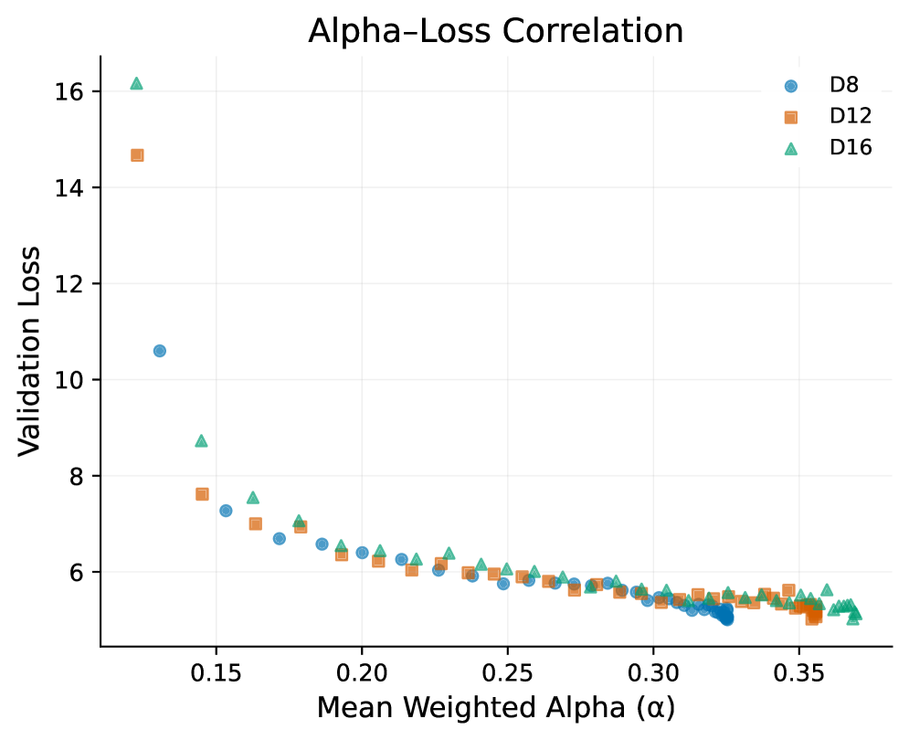
### Visual Description
## Scatter Plot: Alpha-Loss Correlation
### Overview
The image is a scatter plot titled "Alpha-Loss Correlation," visualizing the relationship between **Mean Weighted Alpha (α)** and **Validation Loss** across three datasets (D8, D12, D16). The x-axis represents Mean Weighted Alpha (ranging from 0.1 to 0.35), and the y-axis represents Validation Loss (ranging from 5 to 16). Three distinct data series are plotted using different markers and colors: D8 (blue circles), D12 (orange squares), and D16 (green triangles). The legend is positioned in the top-right corner.
---
### Components/Axes
- **X-axis**: "Mean Weighted Alpha (α)" with ticks at 0.1, 0.15, 0.2, 0.25, 0.3, 0.35.
- **Y-axis**: "Validation Loss" with ticks at 6, 8, 10, 12, 14, 16.
- **Legend**: Located in the top-right corner, mapping:
- Blue circles → D8
- Orange squares → D12
- Green triangles → D16
---
### Detailed Analysis
#### Data Series Trends
1. **D8 (Blue Circles)**:
- Starts at approximately **(0.15, 10.5)**.
- Decreases steadily to **(0.33, 5.2)**.
- Shows a consistent downward trend with minimal scatter.
2. **D12 (Orange Squares)**:
- Begins at **(0.12, 14.8)**.
- Declines to **(0.35, 5.0)**.
- Exhibits a steeper initial drop compared to D8 and D16.
3. **D16 (Green Triangles)**:
- Starts at **(0.1, 16.2)**.
- Reduces to **(0.35, 5.1)**.
- Follows a gradual decline with slight fluctuations.
#### Key Data Points
- **D8**:
- (0.15, 10.5), (0.2, 8.0), (0.25, 6.2), (0.3, 5.5), (0.33, 5.2).
- **D12**:
- (0.12, 14.8), (0.18, 7.0), (0.22, 6.0), (0.28, 5.8), (0.35, 5.0).
- **D16**:
- (0.1, 16.2), (0.15, 8.5), (0.2, 6.5), (0.25, 6.0), (0.3, 5.7), (0.35, 5.1).
---
### Key Observations
1. **Downward Trend**: All three datasets show a clear inverse relationship between Mean Weighted Alpha and Validation Loss. Higher α values correspond to lower validation loss.
2. **Convergence**: By α = 0.3, all datasets cluster tightly between 5.0 and 6.0, suggesting diminishing returns or stabilization of performance at higher α values.
3. **Initial Disparity**: D16 begins with the highest validation loss (16.2 at α = 0.1), while D8 starts lowest (10.5 at α = 0.15). D12 falls in between (14.8 at α = 0.12).
4. **Outliers**: No significant outliers; all points align with their respective trends.
---
### Interpretation
The data suggests that increasing the Mean Weighted Alpha improves model performance (lower validation loss) across all datasets. However, the initial performance disparity (D16 > D12 > D8) indicates inherent differences in dataset complexity or noise. The convergence at higher α values implies that the model's sensitivity to α diminishes as α increases, potentially due to regularization effects or saturation of the model's capacity. This trend could inform hyperparameter tuning strategies, prioritizing higher α values for datasets with initially poor performance (e.g., D16). The uniformity in final performance (α ≥ 0.3) suggests that further increases in α may not yield significant gains, highlighting a trade-off between computational cost and marginal improvements.
</details>
Figure 18: $α$ –loss correlation across models.
<details>
<summary>2604.22778v1/x23.png Details</summary>
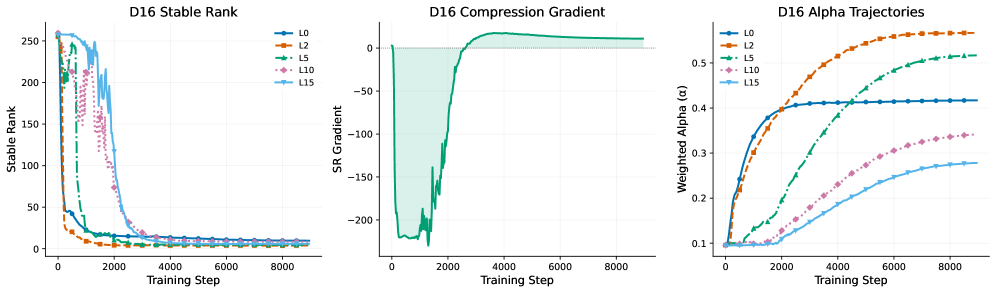
### Visual Description
## Composite Chart: D16 Training Metrics
### Overview
The image contains three sub-charts visualizing training dynamics for a D16 model across different label configurations (L0, L2, L5, L10, L15). Each chart tracks distinct metrics: stable rank convergence, compression gradient behavior, and alpha trajectory evolution. All charts share the same x-axis (Training Step: 0–8000) but differ in y-axis metrics and visualization styles.
---
### Components/Axes
#### Common Elements
- **X-axis**: Training Step (0–8000) across all charts
- **Legend**: Positioned right-aligned in all charts, mapping colors to labels:
- **Blue**: L0
- **Orange**: L2
- **Green**: L5
- **Pink**: L10
- **Light Blue**: L15
#### Chart-Specific Axes
1. **D16 Stable Rank**
- **Y-axis**: Stable Rank (0–250)
- **Line Style**: Solid lines with markers (dots/circles)
- **Shading**: None
2. **D16 Compression Gradient**
- **Y-axis**: SR Gradient (-200–0)
- **Line Style**: Solid green line with shaded uncertainty region (light green)
- **Shading**: Gradient fill between line and zero axis
3. **D16 Alpha Trajectories**
- **Y-axis**: Weighted Alpha (0.1–0.55)
- **Line Style**: Solid lines with markers (dots)
- **Shading**: None
---
### Detailed Analysis
#### D16 Stable Rank
- **Trend**: All lines show rapid initial decline (0–2000 steps), followed by plateauing.
- **L0 (Blue)**: Starts at ~250, drops to ~5 by step 2000, stabilizes near 0.
- **L2 (Orange)**: Similar trajectory to L0 but with slightly slower convergence (~10 by step 2000).
- **L5 (Green)**: Slower decline, stabilizes near ~10.
- **L10 (Pink)**: Gradual decline, stabilizes near ~15.
- **L15 (Light Blue)**: Slowest convergence, stabilizes near ~20.
- **Key Data Points**:
- L0: ~250 (step 0) → ~5 (step 2000) → ~0 (step 8000)
- L15: ~250 (step 0) → ~20 (step 8000)
#### D16 Compression Gradient
- **Trend**: Sharp initial drop to ~-200 (step 1000), followed by rapid ascent to near 0 (step 4000), then stabilization.
- **SR Gradient**: Peaks at ~-200 (step 1000), rises to ~-50 (step 2000), stabilizes near 0 (step 4000+).
- **Uncertainty**: Shaded region widest during initial drop, narrowing post-step 2000.
#### D16 Alpha Trajectories
- **Trend**: All lines show gradual upward curves, with higher labels achieving higher alpha values.
- **L0 (Blue)**: Plateaus near 0.42 by step 8000.
- **L2 (Orange)**: Reaches ~0.55 by step 8000.
- **L5 (Green)**: ~0.48 by step 8000.
- **L10 (Pink)**: ~0.33 by step 8000.
- **L15 (Light Blue)**: ~0.27 by step 8000.
- **Key Data Points**:
- L0: ~0.1 (step 0) → ~0.42 (step 8000)
- L2: ~0.1 (step 0) → ~0.55 (step 8000)
---
### Key Observations
1. **Convergence Speed**: Lower labels (L0, L2) converge faster in stable rank and alpha than higher labels (L10, L15).
2. **Compression Dynamics**: The sharp gradient drop suggests an initial phase of aggressive parameter compression, followed by stabilization.
3. **Alpha Correlation**: Higher labels achieve higher alpha values, indicating better generalization or parameter efficiency.
4. **Uncertainty**: The compression gradient's shaded region implies higher variability in early training steps.
---
### Interpretation
- **Training Efficiency**: Lower labels (L0, L2) demonstrate faster convergence in both stable rank and alpha, suggesting they are more effective for rapid model stabilization.
- **Generalization Trade-off**: Higher labels (L10, L15) achieve higher alpha values but converge more slowly, potentially indicating a trade-off between training speed and generalization.
- **Compression Mechanism**: The compression gradient's behavior implies that the model undergoes significant parameter adjustment early in training, which stabilizes as training progresses.
- **Anomalies**: The pink (L10) and light blue (L15) lines in the stable rank chart show atypical "noise" in early steps, possibly due to label-specific training dynamics.
This data suggests that label configuration significantly impacts training dynamics, with lower labels favoring speed and higher labels favoring generalization. The compression gradient's behavior highlights critical phases of parameter adjustment during training.
</details>
Figure 19: D16 three-panel dynamics.
<details>
<summary>2604.22778v1/x24.png Details</summary>
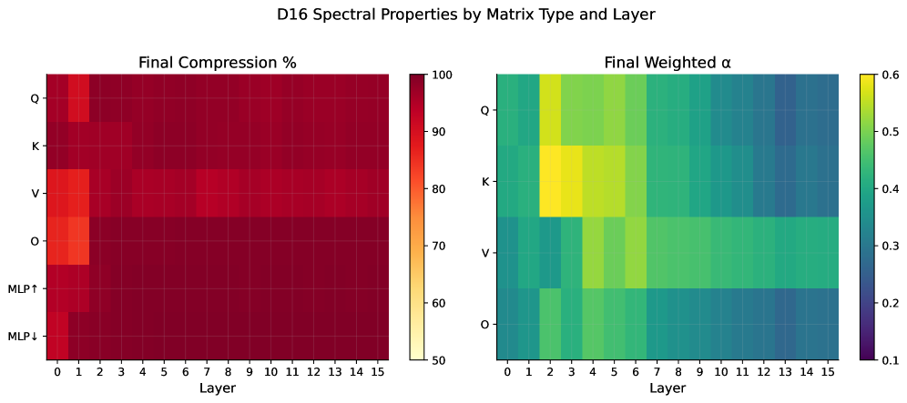
### Visual Description
## Heatmaps: D16 Spectral Properties by Matrix Type and Layer
### Overview
The image contains two side-by-side heatmaps visualizing spectral properties of a D16 model. The left heatmap shows "Final Compression %" (50-100%), while the right shows "Final Weighted α" (0.1-0.6). Both matrices are organized by layer (0-15) on the x-axis and matrix type (Q, K, V, O, MLP↑, MLP↓) on the y-axis.
### Components/Axes
- **X-axis (Layer)**: 0 to 15 (integer increments)
- **Y-axis (Matrix Type)**:
- Q (Query)
- K (Key)
- V (Value)
- O (Other)
- MLP↑ (MLP Up)
- MLP↓ (MLP Down)
- **Color Scales**:
- Left: Dark red (100%) to light yellow (50%)
- Right: Yellow (0.6) to dark purple (0.1)
### Detailed Analysis
#### Final Compression %
- **Q, K, V, O**: Consistently high compression (85-100%) across all layers, with darkest red in layers 0-3.
- **MLP↑/MLP↓**: Lower compression (60-70%), with MLP↓ slightly higher than MLP↑.
- **Layer 0**: All matrix types show peak compression (90-100% for Q/K/V/O).
#### Final Weighted α
- **K**: Highest α values (0.5-0.6) in layers 0-3, dropping to 0.2-0.3 in later layers.
- **Q**: Moderate α (0.3-0.5), peaking in layers 0-2.
- **V**: Lower α (0.2-0.4), with a gradual decline after layer 3.
- **O**: Lowest α (0.1-0.3), minimal variation across layers.
- **MLP↑/MLP↓**: Very low α (0.1-0.2), with MLP↓ slightly higher than MLP↑.
### Key Observations
1. **Early Layer Dominance**: Layers 0-3 exhibit the highest compression and α values for Q/K/V/O.
2. **MLP Layer Consistency**: MLP↑/MLP↓ show minimal variation in both metrics, suggesting stable but low importance.
3. **α Decay**: α values for Q/K/V/O decrease significantly after layer 3, while compression remains high.
### Interpretation
The data suggests that early layers (0-3) of the D16 model are critical for both compression efficiency and spectral importance (α). Q/K/V/O matrices dominate these layers, indicating their role in capturing essential information. MLP layers (↑/↓) are less compressed and have lower α, implying they contribute less to the model's core functionality. The sharp decline in α after layer 3 may reflect diminishing returns in later layers, while sustained high compression suggests efficient parameter sharing or redundancy in later stages. This pattern aligns with typical transformer architectures, where early layers handle semantic features and later layers refine representations.
</details>
Figure 20: D16 matrix type heatmap.
<details>
<summary>2604.22778v1/x25.png Details</summary>
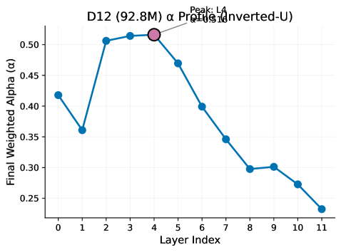
### Visual Description
## Line Graph: D12 (92.8M) α Profile (Inverted-U)
### Overview
The image depicts a line graph illustrating the "Final Weighted Alpha (α)" values across 12 layers (Layer Index 0–11) for a model labeled "D12 (92.8M)". The graph shows a clear inverted-U trend, with a peak at Layer 4 (α = 0.516). The y-axis ranges from 0.25 to 0.50, while the peak value slightly exceeds this range. The line is blue, and the peak is marked with a pink circle and annotated text.
---
### Components/Axes
- **X-Axis (Layer Index)**: Labeled "Layer Index" with integer values from 0 to 11.
- **Y-Axis (Final Weighted Alpha)**: Labeled "Final Weighted Alpha (α)" with values from 0.25 to 0.50 in increments of 0.05.
- **Legend**: Located at the top-left, labeled "D12 (92.8M)" with a blue line.
- **Annotations**:
- Peak at Layer 4 marked with a pink circle.
- Text annotation: "Peak: L4 α = 0.516".
---
### Detailed Analysis
- **Line Data**:
- Layer 0: α ≈ 0.41
- Layer 1: α ≈ 0.36
- Layer 2: α ≈ 0.50
- Layer 3: α ≈ 0.51
- Layer 4: α ≈ 0.516 (peak)
- Layer 5: α ≈ 0.47
- Layer 6: α ≈ 0.40
- Layer 7: α ≈ 0.35
- Layer 8: α ≈ 0.30
- Layer 9: α ≈ 0.30
- Layer 10: α ≈ 0.27
- Layer 11: α ≈ 0.23
- **Trend Verification**:
- The line starts at 0.41 (Layer 0), drops to 0.36 (Layer 1), then rises sharply to 0.516 (Layer 4), followed by a gradual decline to 0.23 (Layer 11). The inverted-U shape is consistent with the annotation.
- **Spatial Grounding**:
- Legend: Top-left corner, blue line.
- Peak annotation: Centered above Layer 4, pink circle with black text.
---
### Key Observations
1. **Peak at Layer 4**: The highest α value (0.516) occurs at Layer 4, slightly exceeding the y-axis maximum (0.50).
2. **Inverted-U Shape**: Values increase from Layer 0 to 4, then decrease monotonically.
3. **Initial Drop**: A sharp decline from Layer 0 (0.41) to Layer 1 (0.36) suggests Layer 1 contributes less than Layer 0.
4. **Post-Peak Decline**: After Layer 4, α decreases by ~0.28 over 7 layers, indicating diminishing returns or negative contributions from deeper layers.
---
### Interpretation
The inverted-U profile suggests that Layer 4 is the optimal layer for the model's performance, as measured by α. This could imply:
- **Layer 4 Specialization**: Layer 4 may encode critical features for the task (e.g., in a neural network).
- **Diminishing Returns**: Deeper layers (5–11) contribute less effectively, possibly due to overfitting, redundancy, or noise.
- **Layer 1 Anomaly**: The drop from Layer 0 to 1 might indicate architectural inefficiencies or suboptimal initialization in early layers.
The data highlights the importance of Layer 4 in the D12 model, warranting further investigation into its role in the model's architecture or training process.
</details>
Figure 21: D12 $α$ profile (inverted-U).
<details>
<summary>2604.22778v1/x26.png Details</summary>
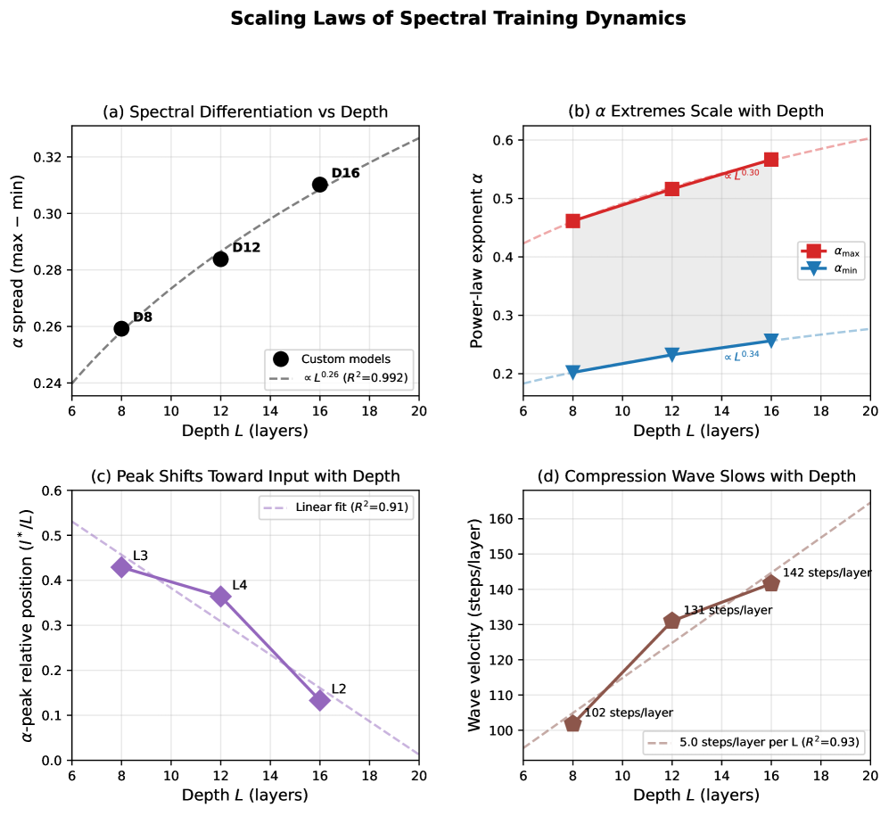
### Visual Description
## Chart: Scaling Laws of Spectral Training Dynamics
### Overview
The image contains four subplots (a-d) illustrating scaling laws of spectral properties in neural networks as a function of network depth. Each subplot demonstrates a distinct spectral dynamic with depth, supported by mathematical fits and annotated data points.
---
### Components/Axes
#### Subplot (a): Spectral Differentiation vs Depth
- **X-axis**: Depth L (layers) [6–20]
- **Y-axis**: α spread (max − min) [0.24–0.32]
- **Legend**:
- Black circles: "Custom models"
- Dashed line: Linear fit (α ≈ L⁰.²⁶, R²=0.992)
- **Data points**:
- D8: α = 0.26
- D12: α = 0.28
- D16: α = 0.30
#### Subplot (b): α Extremes Scale with Depth
- **X-axis**: Depth L (layers) [6–20]
- **Y-axis**: Power-law exponent α [0.2–0.6]
- **Legend**:
- Red squares: α_max
- Blue triangles: α_min
- **Data points**:
- α_max:
- D8: 0.45
- D12: 0.5
- D16: 0.55
- D20: 0.6
- α_min:
- D8: 0.2
- D12: 0.23
- D16: 0.25
- **Fits**:
- α_max: α ≈ L⁰.³⁰ (R²=0.99)
- α_min: α ≈ L⁰.³⁴ (R²=0.98)
#### Subplot (c): Peak Shifts Toward Input with Depth
- **X-axis**: Depth L (layers) [6–20]
- **Y-axis**: α-peak relative position (I*/L) [0–0.6]
- **Legend**:
- Dashed line: Linear fit (R²=0.91)
- **Data points**:
- L2: 0.15
- L3: 0.35
- L4: 0.4
#### Subplot (d): Compression Wave Slows with Depth
- **X-axis**: Depth L (layers) [6–20]
- **Y-axis**: Wave velocity (steps/layer) [100–160]
- **Legend**:
- Dashed line: 5.0 steps/layer per L (R²=0.93)
- **Data points**:
- D8: 102 steps/layer
- D12: 131 steps/layer
- D16: 142 steps/layer
- D20: 160 steps/layer
---
### Detailed Analysis
#### Subplot (a)
- **Trend**: α spread increases monotonically with depth, following a power-law relationship (α ≈ L⁰.²⁶). The fit is exceptionally strong (R²=0.992).
- **Key values**:
- At L=8: α = 0.26
- At L=16: α = 0.30
#### Subplot (b)
- **Trend**:
- α_max increases sharply with depth (α ≈ L⁰.³⁰, R²=0.99).
- α_min increases more gradually (α ≈ L⁰.³⁴, R²=0.98).
- **Key values**:
- At L=8: α_max = 0.45, α_min = 0.2
- At L=16: α_max = 0.55, α_min = 0.25
#### Subplot (c)
- **Trend**: α-peak position decreases linearly with depth (R²=0.91), indicating peaks shift toward input as networks deepen.
- **Key values**:
- At L=2: 0.15
- At L=4: 0.35
- At L=3: 0.4 (peak at L=3)
#### Subplot (d)
- **Trend**: Wave velocity increases linearly with depth (5.0 steps/layer per L, R²=0.93).
- **Key values**:
- At L=8: 102 steps/layer
- At L=16: 142 steps/layer
- At L=20: 160 steps/layer
---
### Key Observations
1. **Consistent Scaling**: All subplots show strong power-law or linear relationships (R² > 0.91), suggesting predictable scaling laws.
2. **Divergent Dynamics**:
- Spectral differentiation (a) and α_max (b) increase with depth.
- α_min (b) and peak position (c) decrease with depth.
- Wave velocity (d) increases with depth.
3. **Depth Sensitivity**: Metrics like α spread (a) and wave velocity (d) show significant changes even between small depth increments (e.g., L=8 to L=12).
---
### Interpretation
The data demonstrates that spectral properties of neural networks scale systematically with depth, governed by power laws or linear relationships. These findings suggest:
- **Design Implications**: Predictable scaling allows for a priori estimation of spectral properties in deeper networks, aiding architectural choices.
- **Training Dynamics**: The compression wave slowing (d) may reflect increased computational complexity per layer in deeper networks.
- **Spectral Trade-offs**: The divergence between α_max and α_min (b) implies that deeper networks amplify certain spectral features while suppressing others, potentially affecting generalization or robustness.
The high R² values (0.91–0.992) validate the reliability of these scaling laws, making them actionable for both theoretical analysis and practical implementation.
</details>
Figure 22: Scaling laws: (a) $Δα$ vs. depth, (b) $α$ extremes, (c) peak position, (d) wave velocity.
<details>
<summary>2604.22778v1/x27.png Details</summary>
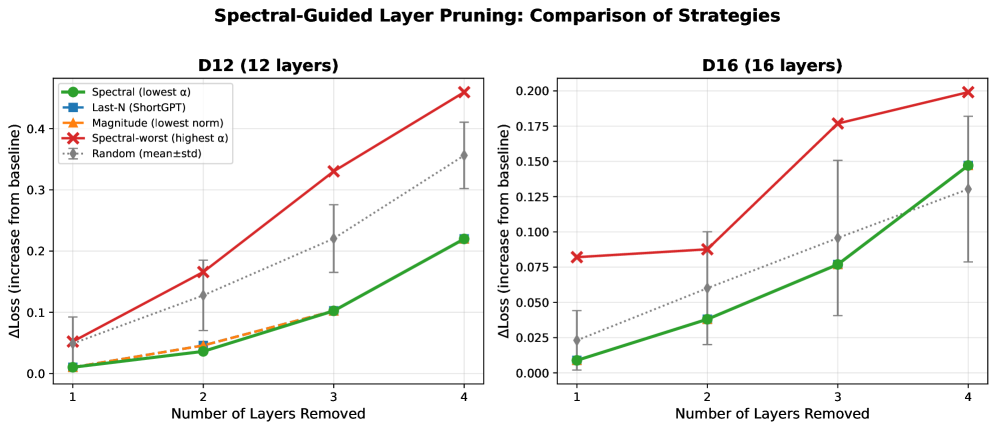
### Visual Description
## Line Chart: Spectral-Guided Layer Pruning: Comparison of Strategies
### Overview
The image compares four layer pruning strategies (Spectral, Last-N, Magnitude, Spectral-worst) and a random baseline across two neural network architectures (D12 with 12 layers and D16 with 16 layers). The y-axis measures the relative increase in loss (ΔLoss) from the baseline, while the x-axis tracks the number of layers removed (1–4). Error bars represent standard deviation.
### Components/Axes
- **Title**: "Spectral-Guided Layer Pruning: Comparison of Strategies"
- **Subplots**:
- Left: D12 (12 layers)
- Right: D16 (16 layers)
- **X-axis**: "Number of Layers Removed" (1–4)
- **Y-axis**: "ΔLoss (increase from baseline)" (0–0.4 for D12, 0–0.2 for D16)
- **Legend** (top-left):
- Spectral (lowest α): Green circles
- Last-N (ShortGPT): Blue squares
- Magnitude (lowest norm): Orange triangles
- Spectral-worst (highest α): Red crosses
- Random (mean±std): Gray diamonds
### Detailed Analysis
#### D12 Subplot (12 layers)
- **Spectral-worst (red crosses)**:
- Starts at ~0.05 (1 layer removed), peaks at ~0.45 (4 layers removed).
- Steep upward trend with error bars increasing from ±0.02 to ±0.04.
- **Spectral (green circles)**:
- Starts near 0, rises to ~0.22 (4 layers removed).
- Error bars: ±0.01 to ±0.03.
- **Last-N (blue squares)**:
- Similar to Spectral but slightly lower (e.g., ~0.18 at 4 layers).
- Error bars: ±0.02 to ±0.04.
- **Magnitude (orange triangles)**:
- Flat line (~0.02–0.03 across all layers).
- Minimal error bars (±0.01).
- **Random (gray diamonds)**:
- Starts at ~0.05, rises to ~0.35 (4 layers removed).
- Error bars: ±0.03 to ±0.05.
#### D16 Subplot (16 layers)
- **Spectral-worst (red crosses)**:
- Starts at ~0.075 (1 layer), peaks at ~0.20 (4 layers).
- Error bars: ±0.03 to ±0.06.
- **Spectral (green circles)**:
- Starts near 0, rises to ~0.15 (4 layers).
- Error bars: ±0.01 to ±0.02.
- **Last-N (blue squares)**:
- Similar to Spectral (~0.13 at 4 layers).
- Error bars: ±0.02 to ±0.04.
- **Magnitude (orange triangles)**:
- Flat line (~0.02–0.03).
- Minimal error bars (±0.01).
- **Random (gray diamonds)**:
- Starts at ~0.025, rises to ~0.13 (4 layers).
- Error bars: ±0.03 to ±0.05.
### Key Observations
1. **Spectral-worst** consistently causes the largest loss increase in both architectures, with steeper slopes in D12.
2. **Spectral** and **Last-N** perform similarly, with Spectral slightly outperforming Last-N in D12.
3. **Magnitude** pruning has negligible impact on loss across all configurations.
4. **Random** pruning shows moderate loss increases, worse than Spectral/Last-N but better than Spectral-worst.
5. D16 (16 layers) exhibits smaller absolute loss increases than D12 (12 layers) for all strategies.
### Interpretation
The data demonstrates that **Spectral-guided pruning (lowest α)** is the most effective strategy, minimizing loss increases during layer removal. **Spectral-worst pruning** (highest α) is the least effective, causing disproportionately large losses, especially in deeper networks (D12). The **Magnitude** strategy’s flat performance suggests it is ineffective for this task. The **Random** baseline’s performance indicates that unguided pruning introduces moderate but predictable degradation. The smaller loss increases in D16 (16 layers) compared to D12 (12 layers) imply that deeper networks may be more resilient to layer removal under these strategies. Error bars highlight increasing uncertainty with more layers removed, particularly for Spectral-worst and Random strategies.
</details>
Figure 23: Pruning strategy comparison (line plots).
<details>
<summary>2604.22778v1/x28.png Details</summary>
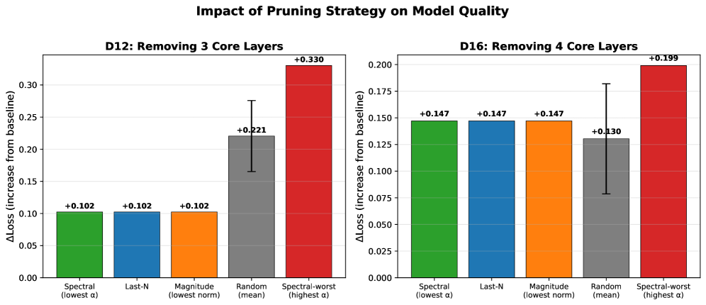
### Visual Description
## Bar Charts: Impact of Pruning Strategy on Model Quality
### Overview
The image contains two side-by-side bar charts comparing the impact of different pruning strategies on model quality. The left chart (D12) focuses on removing 3 core layers, while the right chart (D16) examines removing 4 core layers. Each chart evaluates five pruning strategies: Spectral (lowest α), Last-N, Magnitude (lowest norm), Random (mean), and Spectral-worst (highest α). The y-axis measures ΔLoss (increase from baseline), and error bars indicate variability in results.
### Components/Axes
- **X-Axis (Strategies)**:
- Spectral (lowest α)
- Last-N
- Magnitude (lowest norm)
- Random (mean)
- Spectral-worst (highest α)
- **Y-Axis (ΔLoss)**:
- Scale ranges from 0.00 to 0.35 (D12) and 0.00 to 0.20 (D16).
- **Legends**:
- Colors correspond to strategies:
- Green: Spectral (lowest α)
- Blue: Last-N
- Orange: Magnitude (lowest norm)
- Gray: Random (mean)
- Red: Spectral-worst (highest α)
### Detailed Analysis
#### D12: Removing 3 Core Layers
- **Spectral (lowest α)**: +0.102 (green bar).
- **Last-N**: +0.102 (blue bar).
- **Magnitude (lowest norm)**: +0.102 (orange bar).
- **Random (mean)**: +0.221 (gray bar) with error bar (±0.05).
- **Spectral-worst (highest α)**: +0.330 (red bar).
#### D16: Removing 4 Core Layers
- **Spectral (lowest α)**: +0.147 (green bar).
- **Last-N**: +0.147 (blue bar).
- **Magnitude (lowest norm)**: +0.147 (orange bar).
- **Random (mean)**: +0.130 (gray bar) with error bar (±0.07).
- **Spectral-worst (highest α)**: +0.199 (red bar).
### Key Observations
1. **Spectral-worst (highest α)** consistently shows the largest ΔLoss in both charts, suggesting it is the least effective pruning strategy.
2. **Random (mean)** exhibits significant variability, as indicated by error bars (±0.05 in D12, ±0.07 in D16).
3. **Spectral, Last-N, and Magnitude** strategies yield nearly identical ΔLoss values in both charts, implying similar performance across layer removal counts.
4. ΔLoss increases with the number of layers removed (e.g., D16 values are higher than D12 for equivalent strategies).
### Interpretation
The data suggests that pruning strategies with lower α (Spectral) or norm (Magnitude) are more effective at minimizing ΔLoss compared to Random or Spectral-worst. The Spectral-worst strategy, which targets the highest α values, results in the largest performance degradation, likely due to removing critical features. The Random strategy’s variability (error bars) indicates inconsistent outcomes, possibly due to random selection of layers. The consistent performance of Spectral, Last-N, and Magnitude across both charts implies these methods are robust to changes in the number of layers pruned.
### Spatial Grounding & Trend Verification
- **D12 Chart**:
- Spectral-worst (red) is the tallest bar, confirming it has the highest ΔLoss.
- Random (gray) has the second-highest ΔLoss, with error bars extending to ~0.27.
- **D16 Chart**:
- Spectral-worst (red) again dominates, with ΔLoss of +0.199.
- Random (gray) shows a lower ΔLoss than D12 but higher variability (±0.07).
- **Color Consistency**: All legend colors match bar colors in both charts.
### Uncertainties & Anomalies
- The Random strategy’s error bars suggest measurement noise or variability in layer selection.
- The identical ΔLoss values for Spectral, Last-N, and Magnitude in both charts may indicate a design choice to group these strategies as "effective" pruning methods.
This analysis extracts all textual and numerical data, cross-references legend colors, and interprets trends to explain the relationship between pruning strategies and model quality.
</details>
Figure 24: Pruning strategy comparison (bar charts).