2604.26074v1

# DAK: Direct-Access-Enabled GPU Memory Offloading with Optimal Efficiency for LLM Inference **Authors**: - Shouxu Lin (Cornell University) - Zhiyuan Guo (Cornell University) - Jiaxin Lin (Cornell University) ## Abstract LLM inference is constrained by GPU memory capacity and bandwidth. Tiered memory architectures mitigate this by allowing the GPU to offload memory to the remote tier. However, existing memory offloading frameworks rely on prefetching data into local GPU HBM. This approach underutilizes system resources by introducing HBM contention, squandering memory capacity, and creating pipeline bubbles. We show that enabling direct GPU access to remote memory significantly outperforms prefetching, achieving optimal aggregate system bandwidth. We propose DAK, an end-to-end direct-access memory offloading framework that repurposes the Tensor Memory Accelerator (TMA) to asynchronously fetch offloaded weights and KV caches directly from remote memory into GPU shared memory (SMEM). To maximize remote access performance, DAK introduces a greedy algorithm to determine optimal per-operation offloading ratios, alongside active congestion control and TMA multicast to eliminate interconnect bottlenecks and read amplification. Evaluations across diverse architectures show that DAK achieves near-optimal bandwidth aggregation, with up to 3 $×$ performance gains on NVLink-C2C and 1.8 $×$ on PCIe systems compared to state-of-the-art memory offloading baselines. ## 1 Introduction Large Language Models (LLMs) are increasingly starved for memory capacity and bandwidth due to massive parameter scaling, ultra-long contexts, and large inference batch sizes. Scaling the GPU’s local High Bandwidth Memory (HBM) to meet this demand is prohibitively expensive and fundamentally constrained by die area and thermal limits [gholami2024aimemorywall]. To breach this "memory wall," recent architectures adopt tiered memory designs. By connecting the GPU to remote memory (e.g., host CPU memory via NVLink-C2C or CXL) [li2025fenghuang, fusco2024understanding, cxlconsortium2023spec, nvidia2023gh200arch], these systems decouple compute and memory scaling. For instance, the NVIDIA Grace Hopper (GH200) [nvidia2023gh200arch] utilizes NVLink-C2C to connect the GPU with the CPU memory, which increases the effective memory capacity by 500% and bandwidth by 12.5%. <details> <summary>2604.26074v1/x1.png Details</summary>  ### Visual Description ## Line Graph: Aggregate System Memory Bandwidth vs. Offload Ratio ### Overview The graph illustrates the relationship between effective memory bandwidth (GB/s) and offload ratio (x) for two memory access strategies: **Theoretical Direct Access** and **Theoretical Prefetch**, alongside measured results for "Ours" and "SoTA Prefetch System." Key trends include a sharp decline in bandwidth for both strategies as offload ratio increases, with a notable peak at x=0.1. --- ### Components/Axes - **X-axis**: Offload Ratio (x) ranging from 0.0 to 1.0 in increments of 0.2. - **Y-axis**: Effective Bandwidth (GB/s) ranging from 0 to 3500 in increments of 500. - **Legend**: Located in the top-right corner, with four entries: - **Blue line**: Theoretical Direct Access - **Orange line**: Theoretical Prefetch - **Blue dots**: Ours (Measured) - **Orange crosses**: SoTA Prefetch System (Measured) - **Annotations**: - Red star and arrow highlight the peak at x=0.1 for Theoretical Direct Access. - Red text: "Aggregate system memory bandwidth." --- ### Detailed Analysis 1. **Theoretical Direct Access (Blue Line)**: - Starts at ~3500 GB/s at x=0.0. - Drops sharply to ~400 GB/s at x=1.0. - Peak at x=0.1 (~3500 GB/s), marked by a red star. 2. **Theoretical Prefetch (Orange Line)**: - Starts at ~3000 GB/s at x=0.0. - Declines gradually to ~300 GB/s at x=1.0. - Slope is less steep than Theoretical Direct Access. 3. **Measured Data Points**: - **Ours (Blue Dots)**: - Follows the Theoretical Direct Access line closely but with minor deviations (e.g., ~3000 GB/s at x=0.2 vs. ~3200 GB/s theoretical). - **SoTA Prefetch System (Orange Crosses)**: - Tracks the Theoretical Prefetch line but with slight underperformance (e.g., ~2500 GB/s at x=0.2 vs. ~2800 GB/s theoretical). --- ### Key Observations - **Peak Performance**: Theoretical Direct Access achieves maximum bandwidth (~3500 GB/s) at x=0.1, after which it declines rapidly. - **Divergence**: Theoretical Direct Access outperforms Prefetch at low offload ratios (x < 0.3), but Prefetch maintains higher bandwidth at higher offload ratios (x > 0.5). - **Measured vs. Theoretical**: Both "Ours" and "SoTA Prefetch System" align with their theoretical curves but show minor reductions, likely due to real-world overheads. --- ### Interpretation - **Trade-off Analysis**: The graph highlights a trade-off between offload ratio and bandwidth efficiency. Theoretical Direct Access offers superior bandwidth at low offload ratios but degrades quickly, while Prefetch provides more stable performance at higher offload ratios. - **Practical Implications**: The measured results ("Ours" and "SoTA Prefetch System") validate the theoretical models but suggest room for optimization to minimize the gap between theory and practice. - **Anomaly**: The sharp drop in Theoretical Direct Access after x=0.1 indicates a potential bottleneck or inefficiency in memory access patterns at higher offload ratios. This analysis underscores the importance of balancing offload strategies to maximize system memory bandwidth, with prefetching emerging as a viable alternative for higher offload scenarios. 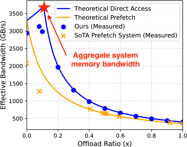</details> Figure 1: Comparison of a prefetch-based system and our direct-access-based system, measured on GH200 with OPT-30b. The central challenge in tiered memory is exploiting remote capacity and bandwidth without suffering interconnect latency penalties. To overcome the challenge of utilizing remote capacity without suffering interconnect latency penalties, prefetching-based frameworks have been proposed. In the context of LLM inference, these frameworks offload a subset of weights and KV caches in remote memory and hide the remote data fetching latencies, with aid of computation-aware prefetching [sheng2023flexgen, kamahori2024fiddler, xu2024pie, vijaya2025aqua, jiang2025neo, kim2025lia, cao2025moe], by analyzing the execution graph and preloading required inputs (weights, and KV caches) from remote memory into GPU HBM before a specific computation block begins. However, we observe that prefetching fundamentally underutilizes both the bandwidth and capacity of tiered memory systems. This bandwidth and capacity underutilization occurs for two reasons. First, prefetching fails to exploit remote bandwidth and leads to degraded local GPU memory bandwidth, as the incoming prefetch traffic (moving data from remote memory to HBM) competes directly with active compute kernels for HBM bandwidth. Second, prefetching limits maximum system memory capacity by forcing data to be staged in local GPU HBM before computation, consuming extra bounce buffers that reduce GPU HBM capacity. Third, prefetching-based approaches are usually coarse-grained (e.g., layer-based [sheng2023flexgen, xu2024pie, kim2025lia]), which seldom achieve perfect overlap between data transfer and computation, leading to pipeline bubbles and low efficiency. Consequently, as shown in Fig. 1, the theoretical performance bound of prefetching falls significantly short of the ideal aggregate system bandwidth (i.e., local GPU HBM plus the host-GPU interconnect). Furthermore, real-world prefetching systems suffer an additional 20% performance degradation due to pipeline bubbles caused by imperfect compute-communication overlap. We argue that enabling the GPU to directly access remote memory can yield significantly better performance than prefetching data through HBM, by allowing GPU Streaming Multi-processors (SMs) to fetch offloaded data directly into shared memory (SMEM). Directly allowing GPU SM’s to access remote memory, we can bypass HBM staging entirely and fully utilize aggregate system bandwidth and capacity, thus reducing both memory and memory bandwidth wastage. In Fig. 1, we show that this direct access mechanism can provide a strictly superior theoretical and empirical performance compared to prefetching. To enable direct access to remote memory, we propose DAK (Direct Access Kernel). Traditionally, a direct data path required GPU threads to explicitly issue load/store instructions over the interconnect, consuming valuable SM register space and instruction cycles. DAK overcomes this by utilizing the Tensor Memory Accelerator (TMA) [nvidia2022hopper], a specialized hardware engine introduced in the Hopper architecture. We observe that, TMA, which was originally designed to manage asynchronous transfers between local HBM and SMEM, can be repurposed to execute asynchronous, direct accesses from remote host memory straight into SMEM. To the best of our knowledge, we are the first to utilize the TMA for remote access and memory offload. However, identifying this hardware capability is only the first step, and we found that a naive implementation of TMA-based remote access is insufficient and can yield non-optimal performance. To make direct remote access achieve near-theoretical maximum performance, we must solve three critical system-level challenges: 1) Determine Offload Ratio: Ignoring the characteristics of memory- and compute-bound kernels in the inference pipeline and blindly offloading memory can underutilize the system. An analytical algorithm is required to determine the optimal offloading ratio for each specific kernel. 2) Interconnect Congestion: We observe that unconstrained in-flight TMA accesses to host memory can trigger severe intra-GPU interconnect congestion and stall the GPU’s local HBM accesses. 3) Uncacheable Host Memory: CPU memory always bypasses the GPU L2 cache (even on coherent architectures like GH200), and uncacheable host memory can cause huge read amplification over interconnects. To solve these challenges, we propose DAK, an end-to-end direct-access memory offloading framework. DAK optimally partitions weights and KV caches across host/GPU memory tiers and employs TMA-enabled warp-specialized kernels to decouple memory fetching from matrix math and efficiently hides heterogeneous memory latencies. DAK overcomes challenges and achieves performance near the theoretical maximum (Fig. 1) with contributions: - Direct Memory Offload Architecture: We develop warp-specialized SplitK_GEMM and SplitK_FlashAttn kernels that compute directly over tiered memory and leverage TMA to fetch offloaded data from remote memory to SMEM. This achieves true bandwidth aggregation, expands memory capacity, and hides remote memory latencies through in-kernel compute-communication overlap. - Optimal Per-operation Offload Ratio: We formulate the memory offloading ratio as a performance optimization problem. We design an efficient greedy algorithm that analytically determines the optimal partitioning ratios for individual compute-bound and memory-bound operations, with provable optimality. - Efficient TMA Access to Host Memory: We identify and mitigate the congestion and read-amplification bottlenecks of naive TMA remote access. We implement active congestion control to prevent host memory requests from stalling local HBM, and we utilize a TMA multicast and host-locality-first tile scheduling to eliminate read amplification for uncacheable host data. - Cross-Architecture Generality: Our direct-access kernels can be adapted across varying interconnect bandwidths (e.g., NVLink-C2C vs. PCIe), distinct GPU architectures, and diverse model configurations, while also ensuring robust performance. 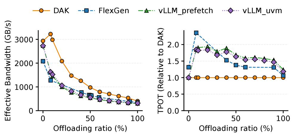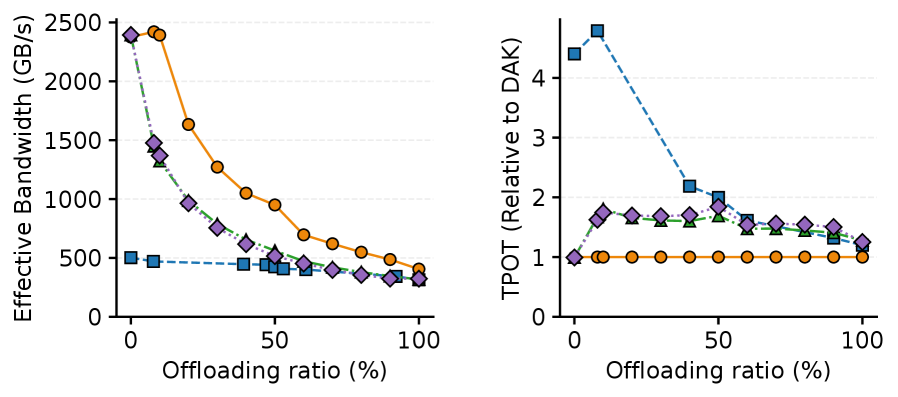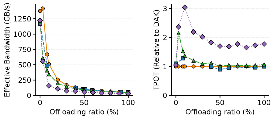We provide a comprehensive evaluation of DAK’s end-to-end effectiveness. DAK is implemented with an accessible PyTorch interface and evaluated across two distinct hardware environments: an NVLink-C2C-based GH200 and a PCIe-based RTX 6000 Blackwell system. We test across multiple models (OPT and Llama) under various batch sizes and sequence length configurations. Compared to multiple state-of-the-art, prefetching-based memory offloading systems, our results show that DAK consistently improves performance across all tested configurations and architectures, delivering up to a 3 $×$ higher throughput on the GH200 and a 1.8 $×$ gain on the RTX 6000 Pro Blackwell. DAK is fully open-sourced at https://github.com/shouxulin/DirectAccessKernel.git. ## 2 Background and Motivation ### 2.1 Scaling Memory with Tiered Architecture The rapid evolution of LLM places unprecedented pressure on memory capacity and bandwidth in inference [kim2024breakthrough, wolters2024memory, alizadeh2024llm]. Memory Capacity bottleneck: Modern LLMs require massive memory capacity for both model weights and KV-Cache. For example, a 671B-parameter model in FP16 requires 1.34 TB of memory for weights alone. At the same time, the KV cache scales linearly with both batch size and sequence length, and can easily exceed 100 GB for a 70B model serving a 100K context at a batch size of 16, rapidly exhausting the GPU’s local HBM capacity. Memory Bandwidth bottleneck: LLM inference requires ultra-high memory bandwidth. For example, during decoding, the entire model weights and the accumulated KV-Cache must be loaded into the computational units for every generated token. This results in low arithmetic intensity, where inference performance is bounded by memory bandwidth [kim2025lia, agrawal2024taming]. <details> <summary>2604.26074v1/x2.png Details</summary>  ### Visual Description ## Diagram: Comparison of GPU Compute Methods (Existing vs. Proposed) ### Overview The diagram compares two methods for GPU compute processes: the **Existing Method (Flexgen)** and **Our Method**. It visualizes the sequence of operations over time, highlighting differences in data transfer, computation, and communication overhead. --- ### Components/Axes - **X-axis**: Labeled "Time" with an arrow pointing right, indicating progression. - **Y-axis**: Two labeled sections: - **Existing Method (Flexgen)** (top) - **Our Method** (bottom) - **Legend** (right side): - **Green blocks**: "Compute Bubbles" (GPU Compute) - **Red blocks**: "Communication Bubbles" - **Blue blocks**: "GPU Compute" (HBM → SM shared mem) - **Key Labels**: - **Existing Method**: - "Weight copy from host (CPU mem → HBM)" - "GPU Compute (HBM → SM shared mem)" - **Our Method**: - "Weight direct access (CPU mem → SM shared mem)" - "GPU Compute (HBM → SM shared mem)" --- ### Detailed Analysis #### Existing Method (Flexgen) 1. **Weight copy from host (CPU mem → HBM)**: - Green block labeled "1" (Compute Bubbles). - Red block labeled "3" (Communication Bubbles). 2. **GPU Compute (HBM → SM shared mem)**: - Blue blocks labeled "0, 1, 2, 3" (GPU Compute). #### Our Method 1. **Weight direct access (CPU mem → SM shared mem)**: - Green blocks labeled "0, 1, 2, 3" (Compute Bubbles). 2. **GPU Compute (HBM → SM shared mem)**: - Blue blocks labeled "0, 1, 2, 3" (GPU Compute). --- ### Key Observations 1. **Reduced Steps in Our Method**: - Eliminates the "Weight copy from host" step (green block "1" and red block "3" in Existing Method). - Direct weight access reduces data transfer latency. 2. **Parallelization**: - Both methods show overlapping GPU compute steps (blue blocks), but Our Method avoids intermediate communication bubbles. 3. **Time Efficiency**: - Our Method’s timeline is shorter due to fewer sequential operations. --- ### Interpretation The diagram demonstrates that **Our Method** optimizes GPU compute workflows by: - **Reducing data transfer overhead**: Direct weight access bypasses the CPU-to-HBM copy step, which introduces communication bubbles (red blocks) in the Existing Method. - **Improving parallelism**: Both methods align GPU compute steps (blue blocks), but Our Method avoids delays caused by intermediate data transfers. - **Enhancing efficiency**: The absence of communication bubbles in Our Method suggests faster execution times and better resource utilization. This comparison highlights the importance of minimizing data movement between memory hierarchies (CPU → HBM → SM) to improve GPU performance. 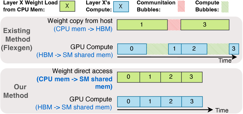</details> Figure 2: Comparing the copy-based method with our method. In FlexGen, layer 1 and 3 weights are offloaded to the CPU. Scaling Memory with Tiered Architecture: An effective strategy to breach this "memory wall" is to allow accelerators access to external memory. This is enabled by the tiered memory, where the GPU is connected to a remote memory tier such as host CPU memory and CXL memory pool [li2023pond, gouk2023memory]. This enables memory resources to scale independently of GPU compute, providing large capacity expansions. This tiered paradigm is also driven by rapid advancements in high-speed compute-memory interconnects like NVLink-C2C [fusco2024understanding, schieffer2024harnessing], die-to-die interconnects [feng2023heterogeneous], and AMD Infinity Fabric [pearson2023interconnect]. For example, in the Grace Hopper (GH200) architecture, the NVLink-C2C connects CPU and GPU with a bandwidth of 450 GB/s per direction, which is close to the host CPU memory bandwidth (500 GB/s). NVLink-C2C increases the GPU’s effective capacity by 500% and expands the total available system memory bandwidth by 12.5% Total available system memory bandwidth is defined by $GPU\_HBM\_BW+MIN(NVLink\_C2C\_BW,HOST\_DRAM\_BW)$ . ### 2.2 Memory Offloading The central research question in tiered memory architectures is how to use remote memory capacity and bandwidth without falling victim to interconnect latency and throughput constraints. Prior work focuses exclusively on using remote memory merely as a capacity pool, managing the data by explicitly copying it between remote memory and GPU local HBM. Paging with Prefetching: Existing works propose general-purpose GPU memory management systems that access remote memory using paging abstractions [sheng2023flexgen, kamahori2024fiddler, kim2025lia, xu2024pie]. These systems rely on prefetching to bring remote pages into the GPU’s local memory before they are needed. Frameworks such as CUDA Managed Memory [li2015evaluation, schieffer2024harnessing] implement prefetching algorithms that copy memory pages from the remote tier into local GPU HBM prior to kernel execution. These prefetching decisions can be triggered either explicitly through programmer-controlled APIs (e.g., cudaMemPrefetchAsync) or implicitly via software- [allen2021depth] or hardware-managed prefetchers [schieffer2024harnessing]. LLM Pipeline Orchestration: Another line of work builds customized GPU kernels or inference pipelines that explicitly control when data is moved from remote memory into local GPU HBM. These systems frame memory offloading as a scheduling optimization problem to maximize the overlap between remote memory communication and active GPU computation. For example, FlexGen [sheng2023flexgen] formulates a linear programming solver to orchestrate model weights and KV cache placement across the GPU, CPU, and disk. To overlap communication with computation, it uses layer-by-layer prefetching. As shown in Fig. 2 (1), while the GPU executes computation for layer $X$ , it concurrently fetches the weights for layer $X+1$ from CPU memory to GPU HBM. Systems like Neo [jiang2025neo] and Lia [kim2025lia] jointly perform memory and computation offloading. Computation offloading is typically beneficial when: (1) operations are strictly memory-bound, making the slower CPU a reasonable alternative, and (2) interconnect bandwidth (e.g., PCIe) is significantly lower than host DRAM bandwidth, and by offloading computation to host can reduce costly data movement across interconnect. However, as next-generation interconnects (e.g., NVLink-C2C in Grace Hopper and Blackwell) achieve bandwidths matching CPU DRAM, the benefits of host-side computation offloading diminish [kamahori2024fiddler, kim2025lia]. <details> <summary>2604.26074v1/x3.png Details</summary>  ### Visual Description ## Diagram: GPU-Host Memory Architecture ### Overview The diagram illustrates the data flow and memory hierarchy between a host system and a GPU, highlighting offload mechanisms and memory components. Key elements include Host DRAM, GPU architecture (SMs, Tensor Core, TMA), Shared Memory (Shared Mem), and High Bandwidth Memory (HBM). Arrows indicate data pathways with distinct styles for different offload types. ### Components/Axes - **Host Side**: - **Host DRAM**: Light blue rectangle labeled "Host DRAM" (top-left). - **Data Paths**: - **Copy Offload Datapath**: Red dotted arrow from Host DRAM to GPU. - **Direct Offload Datapath**: Blue dashed arrow from Host DRAM to GPU. - **GPU Side**: - **SMs**: 6 orange-outlined squares labeled "SM" (arranged in 2 rows of 3). - **Tensor Core/TMA**: - **Tensor/Cuda Core**: Beige rectangle labeled "Tensor / Cuda Core". - **TMA**: Red square labeled "TMA" (adjacent to Tensor Core). - **Shared Mem**: Beige rectangle labeled "Shared Mem" (below Tensor Core/TMA). - **HBM**: Light blue rectangle labeled "HBM" (bottom of GPU). - **Annotations**: - **Arrow 1**: Red arrow pointing to "Shared Mem" (labeled "1"). - **Arrow 2**: Red arrow pointing to "HBM" (labeled "2"). ### Detailed Analysis 1. **Data Flow**: - **Copy Offload (Red Dotted)**: Data moves from Host DRAM to GPU via a slower, indirect path (likely involving CPU mediation). - **Direct Offload (Blue Dashed)**: Data transfers directly from Host DRAM to GPU, bypassing the CPU for lower latency. - **Shared Mem**: Acts as an intermediate buffer between SMs/TMA and HBM, with bidirectional flow (indicated by upward/downward arrows). - **HBM**: Final destination for data processed by SMs/TMA, suggesting high-bandwidth requirements for GPU operations. 2. **Component Hierarchy**: - **SMs**: Core compute units (6 instances) handling parallel workloads. - **TMA**: Specialized for tensor operations, likely accelerating AI/ML tasks. - **Shared Mem**: Managed memory pool for dynamic allocation during GPU computations. - **HBM**: High-speed memory stack feeding data to SMs/TMA. ### Key Observations - **Priority in Data Transfer**: Direct Offload (blue) is prioritized over Copy Offload (red), as indicated by the dashed vs. dotted arrows. - **Memory Tiers**: HBM is positioned as the lowest-latency, highest-bandwidth memory, while Shared Mem serves as a flexible intermediate layer. - **TMA Integration**: The red TMA block is tightly coupled with Tensor Core, emphasizing its role in accelerating matrix operations. ### Interpretation This architecture optimizes GPU offloading by balancing latency and bandwidth: - **Direct Offload** minimizes CPU involvement, critical for real-time applications. - **Shared Mem** acts as a cache, reducing HBM access frequency and improving throughput. - **TMA** suggests specialized hardware for tensor operations, aligning with GPU acceleration in deep learning. - The dual data paths (Copy vs. Direct Offload) imply flexibility for different workload types, with Direct Offload being preferred for performance-sensitive tasks. The diagram underscores a multi-tiered memory hierarchy designed to maximize GPU utilization while managing data movement efficiently between host and accelerator. 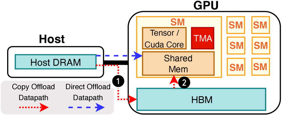</details> Figure 3: Direct memory offload vs. copy data paths. ### 2.3 Limitation of Copy-Based Offloading We observe that all existing copy-based memory offloading solutions are fundamentally suboptimal in utilizing both the bandwidth and capacity of remote memory. Underutilized System Memory Bandwidth. Existing copy-based solutions degrade local GPU memory bandwidth rather than aggregating total system bandwidth. As shown in Fig. 3, the standard datapath requires copying data from the host to HBM (①), and then reading it from HBM to SM shared memory (②). Because HBM is not fully bidirectional, the incoming host writes (①) contend directly with active SM reads (②). In memory-bound kernels, this contention degrades throughput; for example, prefetching layer 1 weights directly interferes with layer 0 computation (Fig. 2). This degradation scales with the interconnect-to-local bandwidth ratio. Background copies can degrade local memory performance by up to 10% on a GH200, and by roughly 4-7% on PCIe-based consumer-grade GPU (64 GB/s PCIe Gen4 vs. 960 GB/s GDDR7) [nvidia2025rtx50series, nvidia2025rtxpro_blackwell_whitepaper]. Communication Bubbles and Wasted HBM Capacity. Copy-based prefetching trade-off between capacity and interconnect utilization. To overlap communication with computation, systems must allocate static HBM staging buffers. As shown in Fig. 2 (1), a naive double-buffered prefetcher will encounters communication bubbles: the interconnect idles while waiting for layer 1’s computation to finish so its buffer can be reused for layer 3. While systems can mask these bubbles by increasing the prefetch depth (e.g., fetching $N$ layers ahead), doing so requires proportionally larger staging buffers, reducing HBM capacity for saving KV cache and weights. Computation Bubbles and Latency Trade-offs. Layer-based coarse-grained prefetching often causes computation bubbles because executing a layer is much faster than fetching its weights (Fig. 2 (1)). To mask these stalls, systems like FlexGen process multiple micro-batches sequentially on the same layer to maximize weight reuse. However, this throughput optimization severely penalizes latency; forcing micro-batches to synchronize at each layer dramatically increases both time-to-first-token and per-token latencies. ### 2.4 Memory Offload with Direct Access To achieve optimal performance, we need for a direct remote-memory-to-SM data path (Fig. 3). Direct access streams data directly from remote memory into the Streaming Multiprocessor’s shared memory (SMEM), bypassing GPU HBM entirely. Traditionally, direct access required GPU threads to explicitly issue load/store instructions over the interconnect, consuming valuable register space and instruction cycles. We overcome this challenge by using the Tensor Memory Accelerator (TMA), a hardware engine introduced after the NVIDIA Hopper architecture. While originally designed for asynchronous transfers between local HBM and SMEM, we novelly prove (§ 6) that TMA can execute asynchronous, direct accesses to remote memory with high-performance. As shown in Fig. 2, this direct-access scheme overcomes the limitations of copy-based methods through three critical benefits: (1) By streaming remote data directly into SMEM, SMs concurrently access host memory and local HBM to achieve the theoretical peak aggregated bandwidth. (2) Eliminating static HBM staging buffers preserves GPU memory for larger models or KV caches. (3) Instead of coarse-grained prefetching, direct access could use asynchronous TMA copies to seamlessly overlap fine-grained kernel computation with remote memory fetches, removing bubbles. <details> <summary>2604.26074v1/x4.png Details</summary>  ### Visual Description ## Diagram: LLaMA 70B + GH200 Memory Offload Architecture ### Overview The diagram illustrates the memory offload strategy for the LLaMA 70B model using a GH200 accelerator. It shows the distribution of model weights between host memory (HBM) and GPU memory, with specific offload ratios (OR) for different weight components. The total offload ratio is 36%, with detailed breakdowns for three key weight types: `qkv_weights`, `kvcache`, and `outproj_weights`. ### Components/Axes - **Left Section**: - **LLaMA 70B**: Model name with ~150GB memory (red text). - **GH200**: Accelerator with 96GB HBM (red text). - **Offload Ratio (OR)**: Total OR = 36% (blue text). - **Right Section**: - **Legend**: - Green squares: Weights on host memory. - Blue squares: Weights on GPU memory. - **Weight Components**: 1. **qkv_weights**: - SplitK_GEMM (OR = 75%). - 12 green (host) + 4 blue (GPU) blocks. 2. **kvcache**: - SplitK_FlashAttn (OR = 25%). - 3 green (host) + 9 blue (GPU) blocks. 3. **outproj_weights**: - SplitK_GEMM (OR = 33%). - 2 green (host) + 6 blue (GPU) blocks. ### Detailed Analysis - **Memory Distribution**: - **qkv_weights**: 75% host (green) vs. 25% GPU (blue). - **kvcache**: 25% host (green) vs. 75% GPU (blue). - **outproj_weights**: 33% host (green) vs. 67% GPU (blue). - **Color Consistency**: - Green blocks in all sections align with the "host memory" legend. - Blue blocks in all sections align with the "GPU memory" legend. - **Spatial Layout**: - LLaMA 70B and GH200 are positioned on the far left. - Arrows point to the three weight components on the right. - Legend is placed at the top-right corner. ### Key Observations 1. **Highest Host Dependency**: `qkv_weights` rely most on host memory (75% OR). 2. **Lowest Host Dependency**: `kvcache` uses the least host memory (25% OR). 3. **Moderate Host Usage**: `outproj_weights` have a balanced split (33% host). 4. **Total Offload Ratio**: The overall OR of 36% suggests a hybrid approach, balancing host and GPU memory usage. ### Interpretation The diagram demonstrates a memory optimization strategy for large language models. By offloading weights to host memory (HBM), the system reduces GPU memory pressure while maintaining performance. The use of **SplitK_GEMM** and **SplitK_FlashAttn** techniques tailors the OR for different weight types: - **qkv_weights** (75% OR): Prioritize host memory for large query-key-value matrices. - **kvcache** (25% OR): Maximize GPU memory for attention cache efficiency. - **outproj_weights** (33% OR): Balance host/GPU usage for output projection layers. The total OR of 36% reflects a system-wide trade-off, leveraging the GH200's 96GB HBM to complement LLaMA's 150GB requirements. This approach highlights the importance of component-specific memory management in large-scale AI inference. 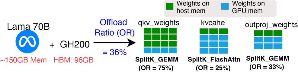</details> Figure 4: DAK overview. ## 3 Overview We build DAK to achieve highly efficient, direct-access memory offloading. The high-level idea of DAK is simple: to fully utilize both local and remote memory, the GPU’s SM should concurrently direct access HBM and host DRAM. This concurrent access is achieved through fine-grained weight partitioning and optimized GPU kernel running on partitioned memory. Fig. 4 shows a high-level overview of DAK. When a user attempts to run a model on a given architecture, memory offloading is required if the available GPU HBM is smaller than the total memory footprint of the model’s weights and KV cache. For example, running a 140 GB model like LLaMA-70B with batch size 32 and sequence length 1024 on a Grace Hopper (GH200) node with 96 GB of HBM requires a global memory offload ratio of 40%. Given this global offload ratio, DAK will calculate the optimal offloading ratio for each individual operation inside the inference pipeline In this paper, we refer to operations involving KV cache matrices as attention (e.g., attention scoring and value aggregation in the attention layer), and operations involving model weights as linear (e.g., the q/k/v/o projections and the gate/up/down projection in MLPs). When we refer to partitioning an operation, we mean partitioning the input matrices of that operation.. Based on these calculated ratios, each operation is partitioned and stored across both the GPU and host memory tiers. After partitioning the operations, DAK invokes optimized, direct-access kernels (e.g., SplitK_GEMM, SplitK_FlashAttn) to execute over the split matrices. These kernels concurrently access local and remote memory. DAK implements a warp-specialized producer-consumer architecture utilizing TMA accelerator for each kernel. This design decouples local/remote memory fetching from matrix math, allowing the GPU SMs to overlap computation with memory latency. Realizing this direct-access architecture introduces many system-level challenges: C1: Optimal Per-Operation Offloading Ratio. How should the system determine the size of data offloaded to host memory for each individual operation, given a global offloading constraint? Different operations exhibit distinct bottlenecks (compute-bound vs. memory-bound), meaning each operation’s performance has a different sensitivity to memory offloading. In 4.2, we formulate this as an optimization problem and design an efficient greedy algorithm that determines per-operation offloading ratios with provable optimality. C2: Managing TMA-based Remote Memory Access. In DAK, GPU SMs concurrently access local and remote memory using the TMA. However, we observe that uncoordinated concurrent accesses can interfere with one another, causing severe intra-GPU interconnect congestion and limiting aggregate bandwidth. Furthermore, CPU memory is non-cacheable by the GPU’s L2 cache (even under the recent cache-coherent Grace Hopper Architecture), requiring the kernel to handle disparate data paths and memory characteristics. In 4.3, we present a congestion control and TMA multicast mechanism that mitigates intra-GPU congestion and handles non-cacheable host memory access. ## 4 Design ### 4.1 DAK Design LLM inference is dominated by matrix multiplication operations, primarily involving the multiplication of hidden states by either model weights or KV cache matrices, in terms of both latency and memory footprint. DAK partitions these operations across both GPU and host memory. Next, we introduce this partitioning scheme and the specialized kernels that compute directly over these partitioned matrices. <details> <summary>2604.26074v1/x5.png Details</summary>  ### Visual Description ## Diagram: Matrix Operation Workflow with GPU Memory Partitioning ### Overview The diagram illustrates a three-stage matrix computation workflow involving host and GPU memory partitioning. It shows how matrix A (weights) is split between host and GPU memory, multiplied with matrix B (hidden) in GPU memory, and stored as matrix C (hidden) in GPU memory. Color-coded tiles represent data partitioning and computation stages. ### Components/Axes 1. **Matrix A (Weights: MxK)** - Dimensions: M rows × K columns - Spatial Partitioning: - Top-left "tile chunk" (red): Host memory (25% offload ratio) - Remaining cells (purple/green/blue): GPU memory - Labels: - Vertical axis: M (rows) - Horizontal axis: K (columns) 2. **Matrix B (Hidden: KxN)** - Dimensions: K rows × N columns - Entirely stored in GPU memory - Labels: - Vertical axis: K (columns from Matrix A) - Horizontal axis: N (columns) 3. **Matrix C (Hidden: MxN)** - Dimensions: M rows × N columns - Entirely stored in GPU memory - Color-coded tiles: - Red: t₀, t₁ - Purple: t₂, t₃ - Green: t₄, t₅ - Blue: t₆, t₇ 4. **Memory Architecture** - Host memory: Top section with red tile chunk - GPU memory: Bottom section with partitioned matrices 5. **Legend** - Located on the right side - Color mapping: - Red: "tile chunk" (host memory) - Purple/Green/Blue: GPU memory partitions ### Detailed Analysis - **Matrix A Partitioning** - 25% of Matrix A (red tile chunk) remains in host memory - 75% of Matrix A (purple/green/blue) offloaded to GPU memory - Spatial distribution: Top-left quadrant as host memory portion - **Matrix Multiplication Flow** - Matrix A (GPU portion) × Matrix B (GPU) → Matrix C (GPU) - Dimensions compatibility: (MxK) × (KxN) = (MxN) - **Matrix C Tile Structure** - 8 total tiles (t₀-t₇) arranged in 4 color groups - Each color group contains 2 adjacent cells - Tiles organized in 2x4 grid (2 columns × 4 rows) ### Key Observations 1. **Memory Optimization** - 25% host memory retention suggests selective offloading strategy - GPU memory handles 75% of computation-intensive data 2. **Computation Pattern** - Tile-based processing evident in Matrix C's color-coded structure - Suggests parallel computation across color-coded tile groups 3. **Dimensional Consistency** - Matrix B's K dimension matches Matrix A's K dimension - Matrix C inherits M (rows) from A and N (columns) from B ### Interpretation This diagram demonstrates a hybrid computation strategy where: 1. **Selective Offloading**: Only 25% of weight matrix (A) remains on host, while 75% is GPU-accelerated 2. **Tile-Based Computation**: Matrix C's color-coded tiles indicate parallel processing units or computation chunks 3. **Memory Hierarchy Awareness**: Explicit distinction between host and GPU memory storage patterns 4. **Dimensional Optimization**: Matrix B's K dimension acts as a bridge between A's columns and C's rows The workflow suggests an optimized matrix multiplication pipeline for deep learning operations, balancing host-GPU memory usage while maintaining dimensional compatibility across matrix operations. The tile-based approach in Matrix C implies potential for parallel processing across different color-coded computation units. </details> (a) Matrices partitioned between host and GPU memory. <details> <summary>2604.26074v1/x6.png Details</summary>  ### Visual Description ## Diagram: GPU Memory Hierarchy and Execution Flow ### Overview This diagram illustrates the memory hierarchy and execution flow in a GPU computing system. It depicts the interaction between Host Memory, Shared Memory, GPU Memory, and execution stages (t_0 to t_7). Key components include a Transactional Memory Array (TMA), Warps (producer/consumer), and Shared Memory slots. The diagram uses color-coded sections to differentiate memory types and execution phases. ### Components/Axes 1. **Host Memory**: Pink section at the bottom, labeled "Host Memory." 2. **Shared Memory**: Gray section above Host Memory, labeled "Shared Memory" with two slots (slot 0 and slot 1). 3. **GPU Memory**: Gray section on the right, labeled "GPU Memory." 4. **Warps**: Top-left section labeled "Warps," containing "producer" and "consumer" blocks. 5. **TMA**: Red block connected to Shared Memory, labeled "TMA." 6. **Execution Stages**: Vertical timeline on the right with seven stages (t_0 to t_7), color-coded: - **t_0**: Red (SM 0) - **t_1**: Pink (SM 1) - **t_2–t_3**: Purple (SM 2–3) - **t_4–t_5**: Green (SM 4–5) - **t_6–t_7**: Blue (SM 6–7) 7. **Arrows**: Blue arrows indicate data flow between components. ### Detailed Analysis - **Host Memory**: Serves as the source for data transfers, connected to Shared Memory via TMA. - **Shared Memory**: Acts as an intermediate buffer between Host Memory and GPU Memory. Contains two slots (slot 0 and slot 1) for temporary data storage. - **TMA**: Facilitates data movement between Host Memory and Shared Memory, highlighted in red. - **Warps**: Represent parallel processing units. The "producer" writes data to Shared Memory, while the "consumer" reads from it. - **Execution Stages**: Sequential phases (t_0 to t_7) are color-coded to indicate progression through the GPU pipeline. Each stage corresponds to a specific memory type (SM 0–7). ### Key Observations - **Color Coding**: - Red (t_0) and pink (t_1) represent early execution stages tied to Host/Shared Memory. - Purple (t_2–t_3), green (t_4–t_5), and blue (t_6–t_7) indicate later stages in GPU Memory. - **Data Flow**: - Data moves from Host Memory → TMA → Shared Memory → Warps (producer/consumer) → GPU Memory. - Arrows suggest bidirectional communication between Shared Memory and Warps. - **Execution Parallelism**: - Multiple execution stages (t_0–t_7) imply concurrent processing across GPU cores. ### Interpretation This diagram models a GPU's memory hierarchy and execution pipeline, emphasizing data movement and parallelism. The TMA acts as a bridge between Host and Shared Memory, optimizing data transfers. Warps enable parallel producer-consumer operations within Shared Memory, while the color-coded execution stages reflect the GPU's phased processing of data. The absence of numerical values suggests this is a conceptual model rather than a performance benchmark. The system highlights the importance of efficient memory management in GPU computing, with Shared Memory serving as a critical intermediate layer for reducing latency between Host and GPU Memory. </details> (b) Kernel on partitioned memories; tile rows executed by different SMs. Figure 5: DAK partitions and executes a matrix multiplication. 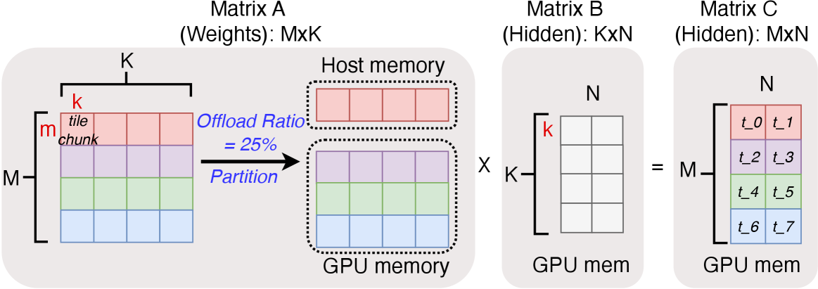Data Partition: Figure 5 illustrates how DAK partitions a matrix multiplication operation, defined as $C=A× B$ , where $C$ and $B$ represent hidden states, and $A$ represents the model weights or KV cache. As shown in 5(a), $A$ is partitioned along the $M$ dimension into multiple tile rows, each of shape $m× K$ . These tile rows are then distributed across host memory and GPU memory. In the example shown, tile row $0$ resides in host memory, while tile rows $1$ through $3$ reside in GPU memory. The optimal number of tiles to be placed in host memory is determined by the offloading algorithm (detailed in § 4.2). 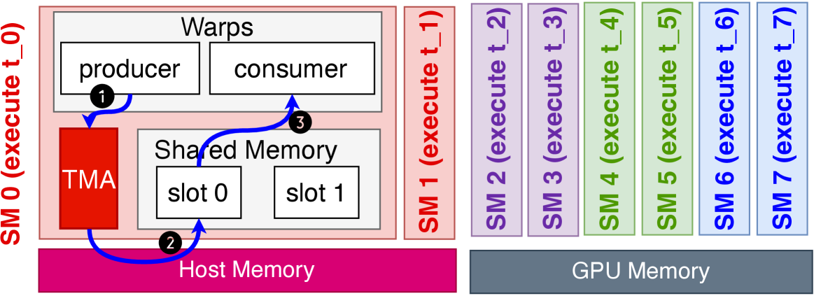Kernel over Partitioned Memory: DAK performs matrix computation directly over this partitioned memory. 5(b) shows this kernel design. Each tile chunk in the output matrix is calculated by a different GPU SM. If the total number of tiles exceeds the available SM count, each SM processes multiple tile chunks. In this example, SMs 0 and 1 handle the computation for output tiles $t_0$ and $t_1$ respectively by reading weights from CPU host memory, while SMs 2 through 7 compute output tiles $t_2$ through $t_7$ by reading weights from local GPU memory. This design strictly isolates the data path, guaranteeing that each individual SM reads exclusively from either host or GPU memory. The number SMs assigned to handle host versus GPU tiles is determined by three factors: (1) the target offloading ratio, which dictates the total size of data that must be processed from each memory tier; (2) execution wave alignment, which ensures the number of assigned tiles evenly divides across the allocated SMs to prevent tail latencies caused by partial, unbalanced execution waves; and (3) interconnect congestion control, which caps the number of host-assigned SMs when necessary to avoid memory contention (detailed in § 4.3). Asynchronous TMA Access: The primary challenge of this approach is efficiently hiding the data load latencies that arise when SMs fetch matrices from HBM or remote host memory. To overlap data movement with computation, DAK adopts a warp-specialized producer-consumer design within each SM, leveraging the Tensor Memory Accelerator (TMA). Since TMA load and store execute asynchronously, data movement happens in the background while Tensor Cores and CUDA cores perform mathematical operations. As shown in 5(b), thread blocks in each SM utilize this warp specialization to mask memory latencies. The execution pipeline proceeds as follows: First, the producer warp leverages the TMA to asynchronously fetch a tile chunk of $A$ from host memory and its corresponding chunk of $B$ from GPU memory into a shared memory (SMEM) slot (Steps ① and ②). Once the slot is filled, the consumer warp performs the matrix multiplication (Step ③). Concurrently, the producer issues the next TMA requests to fetch the subsequent chunks into an alternate SMEM slot. The maximum number of in-flight TMA requests is determined by the available slot number and the congestion control algorithm introduced in § 4.3. By maintaining multiple in-flight TMA requests, the kernel effectively overlaps memory loads with computation. With this design, DAK achieves two critical benefits. First, it enables true parallel execution across memory tiers; by having distinct SMs read from host and GPU memory in parallel, the system fully achieve the aggregate bandwidth of both the local HBM and the host-GPU interconnect. Second, it efficiently absorbs the severe latency penalties of remote data loads through its asynchronous, warp-specialized nature. ### 4.2 Offloading Algorithm This section introduces our offloading algorithm, which optimally distributes a global offloading budget across operations in LLM inference pipeline. We first demonstrate that applying a uniform offloading ratio across operations is suboptimal. To address this, we design a greedy offloading algorithm with provable optimality. #### 4.2.1 The Suboptimality of Uniform Offloading Given a global offloading ratio $OR$ (determined by total memory footprint and available GPU memory), the system must distribute this budget across individual operations. A naive approach is to apply a uniform offloading ratio, where every operation offloads exactly $OR$ fraction of its involving matrices to the host. But this strategy is suboptimal because inference consists of a mixture of memory-bound and compute-bound operations, with different sensitivities to offloading. Diverse Performance Bottlenecks: An operation is memory-bound if its arithmetic intensity (AI) falls below the hardware’s peak machine balance, and compute-bound otherwise. In LLM inference, the performance bottleneck—whether memory- or compute-bound—varies across operations and depends on workload characteristics such as batch size ( $B$ ) and sequence length ( $L$ ). Both prefilling and decoding consist of a mixture of memory-bound and compute-bound operations: - Decoding: The attention operation is strictly memory-bound, as both its computation and memory traffic scale as $O(B· L· D_h)$ ( D_h is the head dimension), yielding a constant Arithmetic Intensity (AI) of $O(1)$ . In contrast, linear operations can be either memory- or compute-bound; it transitions from memory to compute-bound as $B$ grows. - Prefilling: The attention operation can be either memory- or compute-bound: its computation scales quadratically with sequence length ( $O(B· L^2· D_h)$ ) while memory scales linearly ( $O(B· L· D_h)$ ), yielding an AI of $O(L)$ that shifts to compute-bound for long sequences. Linear operations achieve an AI of $O(B· L)$ and remain inherently compute-bound since $B· L$ is large in typical prefilling workloads. <details> <summary>2604.26074v1/x7.png Details</summary>  ### Visual Description ## Line Graph: Effective Bandwidth vs. Offloading Ratio ### Overview The graph illustrates the relationship between effective bandwidth (EB) and offloading ratio, distinguishing between memory-bound and compute-bound scenarios. Two regions (Region 1 and Region 2) are highlighted, with distinct trends for memory and compute-bound systems. ### Components/Axes - **Y-Axis (Effective Bandwidth (EB))**: - Labels: `Bg + Bh`, `Bg`, `Bh`, `Bi = Ci / T_comp` - Scale: Linear, with key thresholds marked. - **X-Axis (Offloading Ratio)**: - Labels: `Bh / (Bh + Bg)`, `Bh / Bi` - Scale: Linear, with critical ratios annotated. - **Legend**: - Top-right placement. - Colors: - Blue: Memory-bound - Red: Compute-bound - Red hatch: Region 1 - Green hatch: Region 2 ### Detailed Analysis 1. **Memory-bound Curve (Blue)**: - Starts at `Bg + Bh` (peak) and declines exponentially. - Intersects the `Bg` threshold at `Bh / (Bh + Bg)` offloading ratio. - Crosses `Bi = Ci / T_comp` at `Bh / Bi` offloading ratio. 2. **Compute-bound Curve (Red)**: - Begins at `Bg` and decreases gradually. - Overlaps with the memory-bound curve at `Bh / Bi` offloading ratio. - Flattens near `Bh` threshold. 3. **Regions**: - **Region 1 (Red hatch)**: - Bounded by `Bg` to `Bg + Bh` bandwidth and `0` to `Bh / (Bh + Bg)` offloading ratio. - **Region 2 (Green hatch)**: - Bounded by `Bg` to `Bg + Bh` bandwidth and `Bh / (Bh + Bg)` to `Bh / Bi` offloading ratio. ### Key Observations - The memory-bound system achieves higher bandwidth at low offloading ratios but degrades sharply beyond `Bh / (Bh + Bg)`. - Compute-bound performance remains stable until `Bh / Bi`, after which it declines. - The intersection at `Bh / Bi` suggests a critical transition point between memory and compute bottlenecks. - Region 1 (low offloading) is dominated by memory constraints, while Region 2 (high offloading) shifts to compute limitations. ### Interpretation The graph demonstrates that offloading ratio directly impacts system performance, with memory-bound systems excelling at low offloading and compute-bound systems taking over at higher ratios. The critical thresholds (`Bh / (Bh + Bg)` and `Bh / Bi`) define operational boundaries for optimizing resource allocation. The exponential drop in memory-bound bandwidth highlights diminishing returns beyond a certain offloading point, while the compute-bound curve’s gradual decline suggests scalability limits in computational resources. This analysis is critical for designing hybrid systems that balance memory and compute offloading to maximize effective bandwidth. </details> Figure 6: Effective bandwidth of memory/compute-bound operations. 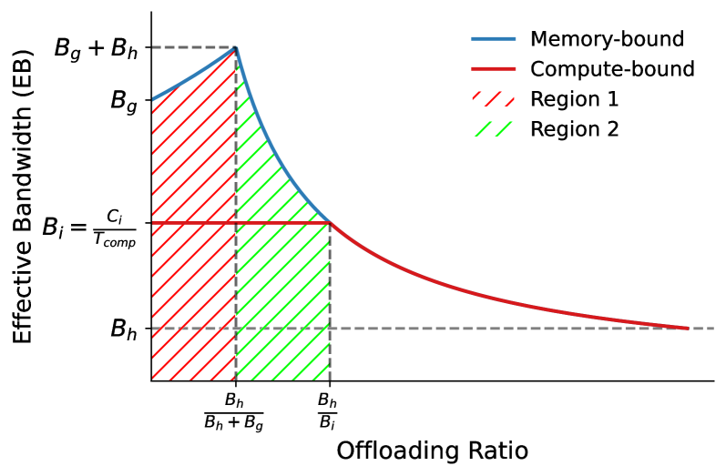Different Sensitivities to Offloading: Memory/compute-bound operations react differently to the offloading ratio. To quantify this, we use the Effective Bandwidth ( $EB$ ) as the performance metric, which is defined as the total fetched data from memory ( $C$ ) $C$ is the size of model weights or KV cache for linear or attention. divided by the overall operation execution latency: $EB=\frac{C}{\max(T_comp,T_mem)}$ , where $T_comp$ is the computation time and $T_mem$ is the memory access time. Fig. 6 shows how $EB$ of both compute- and memory-bound kernels changes as the offloading ratio increases. We use $EB$ as the primary performance metric because it provides a unified standard to easily identify whether an operation is memory- or compute-bound. - Memory-bound operations ( $T_comp<T_mem$ ): The operation performance is bounded by $T_mem$ . Because DAK concurrently reads from both host and GPU memory, the overall memory latency is bounded by the slower of the two transfers: $T_mem=\max(T_h,T_g)$ , where $T_h$ and $T_g$ are the host and GPU data transfer times, respectively. As shown in the figure, $EB$ initially increases with the offloading ratio, reaches a peak, and then decreases. This peak EB occurs at an optimal ratio of $\frac{B_h}{B_h+B_g}$ , where $B_h$ and $B_g$ denote the host interconnect bandwidth and GPU memory bandwidth. At this threshold, the data transfer times are perfectly balanced ( $T_h=T_g$ ). Consequently, the operation fully utilizes both memory bandwidths simultaneously. However, if the offloading ratio is beyond this point, reading from the slower host interconnect ( $T_h$ ) becomes the bottleneck, and performance degrades. - Compute-bound operations ( $T_comp>T_mem$ ): For these operations, $EB$ remains flat initially, since at lower offloading ratios, the operation latency is strictly dominated by the mathematical computation time ( $T_comp$ ) rather than memory time. Because the computation effectively hides the memory transfer latency, offloading weights to the host does not impact the overall EB. However, this flat trend only holds up to a critical threshold (which we refer to as the “threshold” of compute-bound operations). Beyond this point, data movement from host memory becomes the bottleneck (i.e., when $T_mem=T_h≥ T_comp$ ). Once this threshold is crossed, the operation transitions into a memory-bound regime dictated by the host interconnect, and $EB$ begins to decrease following the same behavior as the memory-bound case. Suboptimality of Uniform Offloading: A uniform method that assigns the same ratio $r$ to all operations will be suboptimal. As shown in Fig. 6, the suboptimal show up in two regions. Region 1 ( $r≤\frac{B_h}{B_h+B_g}$ ): the memory-bound operation is starved and actively benefits from increasing its offloading ratio toward its optimal peak, thus the offloading ratio for compute-bound operations should be allocated to memory-bound operations. Region 2 ( $\frac{B_h}{B_h+B_g}<r<\frac{B_h}{B_i}$ ): memory-bound operations suffer from effective bandwidth loss due to offloading. While compute-bound operations are still insensitive, the offloading budget should be shifted from memory-bound operations to compute-bound operations. #### 4.2.2 Optimal Greedy Offload Because varying operations yield different performance curves, we formulate this ratio offloading allocation as an optimization problem. Problem Formulation: Say the global offload ratio is $OR$ . Given a set of operations $F$ , we assign an offloading ratio $x_i∈[0,1]$ to each operation $F_i$ . The sum of offloaded data from all operations should match the global ratio constraint. Our objective is to minimize the end-to-end execution time, which is the sum of individual operation latencies. Using the effective bandwidth model, the latency of operation $F_i$ can be written as $\frac{C_i}{EB(x_i)}$ under offloading ratio $x_i$ . Greedy Offload Algorithm: We prove that the optimal allocation strictly follows a multi-stage greedy algorithm based on each operator’s turning point shown in Fig. 6. We allocate the offloading ratio to operations in three distinct phases: - Allocate to Memory-Bound Operations. It first allocates the offloading budget all to memory-bound operations, since it directly improves $EB$ . The exact distribution of the budget between the memory-bound operations does not matter if no memory operation’s ratio is beyond its turning point. - Saturate Compute-Bound Operations. Once all memory-bound operations reach their peak $EB$ , the remaining offloading budget should be distributed to the compute-bound operations. Similar to the first phase, the exact distribution among compute-bound operations does not affect optimality, as long as no compute-bound operation’s ratio is beyond its turning point. - Arbitrary Allocation. If the global offloading ratio is large enough that all operations (both memory- and compute-bound) have reached their turning points, the remaining budget can be assigned arbitrarily across any operations without affecting the end-to-end latency. Proof of Optimality: We prove via contradiction (Appendix A) that our greedy algorithm is optimal. <details> <summary>2604.26074v1/x8.png Details</summary>  ### Visual Description ## Line Chart: Memory Access Bandwidth vs. Number of SM Hosts ### Overview The chart illustrates the relationship between the number of SM hosts (`N_SM_Host`) and three types of memory access bandwidth: SM-to-host, SM-to-HBM, and Aggregate Bandwidth. The y-axis represents bandwidth in GB/s, while the x-axis represents the number of SM hosts, ranging from 12 to 32. ### Components/Axes - **X-axis (Horizontal)**: Labeled `N_SM_Host`, with values at 12, 4, 8, 16, 24, and 32. - **Y-axis (Vertical)**: Labeled `Memory Access Bandwidth (GB/s)`, ranging from 0 to 4000. - **Legend**: Located in the bottom-left corner, with three entries: - **Blue squares**: SM-to-host Bandwidth - **Orange triangles**: SM-to-HBM Bandwidth - **Green circles**: Aggregate Bandwidth ### Detailed Analysis 1. **SM-to-host Bandwidth (Blue Squares)**: - Starts at ~100 GB/s for `N_SM_Host = 12`. - Increases to ~400 GB/s at `N_SM_Host = 8`. - Remains relatively stable (~400 GB/s) for `N_SM_Host = 16, 24, 32`. 2. **SM-to-HBM Bandwidth (Orange Triangles)**: - Begins at ~3500 GB/s for `N_SM_Host = 12`. - Decreases steadily to ~3000 GB/s at `N_SM_Host = 32`. 3. **Aggregate Bandwidth (Green Circles)**: - Starts at ~3500 GB/s for `N_SM_Host = 12`. - Peaks at ~3800 GB/s at `N_SM_Host = 8`. - Declines to ~3300 GB/s at `N_SM_Host = 32`. ### Key Observations - **SM-to-host Bandwidth** shows a sharp increase until `N_SM_Host = 8`, then plateaus. - **SM-to-HBM Bandwidth** decreases linearly as `N_SM_Host` increases. - **Aggregate Bandwidth** peaks at `N_SM_Host = 8` before declining, suggesting diminishing returns beyond this point. ### Interpretation The data suggests that increasing the number of SM hosts initially improves SM-to-host bandwidth but does not scale linearly beyond 8 hosts. Conversely, SM-to-HBM bandwidth decreases with more hosts, possibly due to resource contention or architectural limitations. The Aggregate Bandwidth peaks at 8 hosts, indicating an optimal configuration for total memory access efficiency. Beyond this point, adding more SM hosts reduces overall performance, highlighting a trade-off between scalability and bandwidth efficiency. **Notable Anomaly**: The Aggregate Bandwidth’s peak at `N_SM_Host = 8` contrasts with the SM-to-HBM trend, suggesting a bottleneck or optimization in the system’s design at this specific configuration. </details> (a) $N\_inflight=3$ , $N_SM\_HBM=100$ and we vary $N_SM\_Host$ . <details> <summary>2604.26074v1/x9.png Details</summary>  ### Visual Description ## Line Graph: Memory Access Bandwidth vs. N_inflight ### Overview The graph illustrates the relationship between memory access bandwidth (GB/s) and the number of inflight operations (N_inflight) across three data series: SM-to-host Bandwidth, SM-to-HBM Bandwidth, and Aggregate Bandwidth. The y-axis represents bandwidth in GB/s, while the x-axis ranges from N_inflight = 1 to 6. ### Components/Axes - **X-axis (N_inflight)**: Integer values from 1 to 6, labeled "N_inflight". - **Y-axis (Memory Access Bandwidth)**: Scale from 0 to 4000 GB/s, labeled "Memory Access Bandwidth (GB/s)". - **Legend**: Located in the top-right corner, with three entries: - **Blue squares**: SM-to-host Bandwidth - **Orange triangles**: SM-to-HBM Bandwidth - **Green circles**: Aggregate Bandwidth ### Detailed Analysis 1. **SM-to-host Bandwidth (Blue Squares)**: - **Trend**: Flat line at approximately 200 GB/s across all N_inflight values (1–6). - **Data Points**: Consistent at ~200 GB/s, with no variation. 2. **SM-to-HBM Bandwidth (Orange Triangles)**: - **Trend**: Increases sharply from N_inflight = 1 to 3, peaks at N_inflight = 3 (~3500 GB/s), then declines to ~3000 GB/s at N_inflight = 6. - **Data Points**: - N_inflight = 1: ~1900 GB/s - N_inflight = 2: ~3300 GB/s - N_inflight = 3: ~3500 GB/s - N_inflight = 4: ~3400 GB/s - N_inflight = 5: ~3250 GB/s - N_inflight = 6: ~3000 GB/s 3. **Aggregate Bandwidth (Green Circles)**: - **Trend**: Mirrors SM-to-HBM but with higher values. Peaks at N_inflight = 3 (~3800 GB/s), then declines to ~3200 GB/s at N_inflight = 6. - **Data Points**: - N_inflight = 1: ~2000 GB/s - N_inflight = 2: ~3500 GB/s - N_inflight = 3: ~3800 GB/s - N_inflight = 4: ~3600 GB/s - N_inflight = 5: ~3450 GB/s - N_inflight = 6: ~3200 GB/s ### Key Observations - **SM-to-host Bandwidth** remains constant regardless of N_inflight. - **SM-to-HBM Bandwidth** and **Aggregate Bandwidth** exhibit a peak at N_inflight = 3, followed by a decline. - **Aggregate Bandwidth** consistently exceeds SM-to-HBM Bandwidth by ~200–500 GB/s across all N_inflight values. - The sharpest increase in bandwidth occurs between N_inflight = 1 and 2 for both SM-to-HBM and Aggregate. ### Interpretation The data suggests that memory access bandwidth is highly sensitive to N_inflight up to a critical point (N_inflight = 3), after which performance degrades. The Aggregate Bandwidth likely represents a combined or optimized utilization of SM-to-HBM and SM-to-host resources, as it consistently outperforms SM-to-HBM alone. The flat SM-to-host Bandwidth indicates it is decoupled from N_inflight, possibly due to fixed hardware constraints. The peak at N_inflight = 3 may reflect optimal parallelism or resource allocation, while the subsequent decline could signal contention or saturation in memory access pathways. </details> (b) $N_SM\_HOST=8$ , $N_SM\_HBM=100$ and we vary $N\_inflight$ . Figure 7: Local/remote memory access congestion on GH200. Increased $N_SM\_Host$ or $N_inflight$ reduces SM-to-HBM bandwidth. ### 4.3 Efficient Host Memory Access with TMA In DAK, SMs utilize the TMA to concurrently access both host and GPU memory. To our knowledge, DAK is the first system to leverage TMA for host memory accesses. However, relying on TMA for cross-interconnect data movement requires careful orchestration to achieve optimal performance and avoid severe resource contention. #### 4.3.1 Congestion Control over Local/Remote Access We observe that issuing an unconstrained number of inflight TMA requests to host memory triggers interconnect congestion, which degrades the GPU’s local HBM performance. 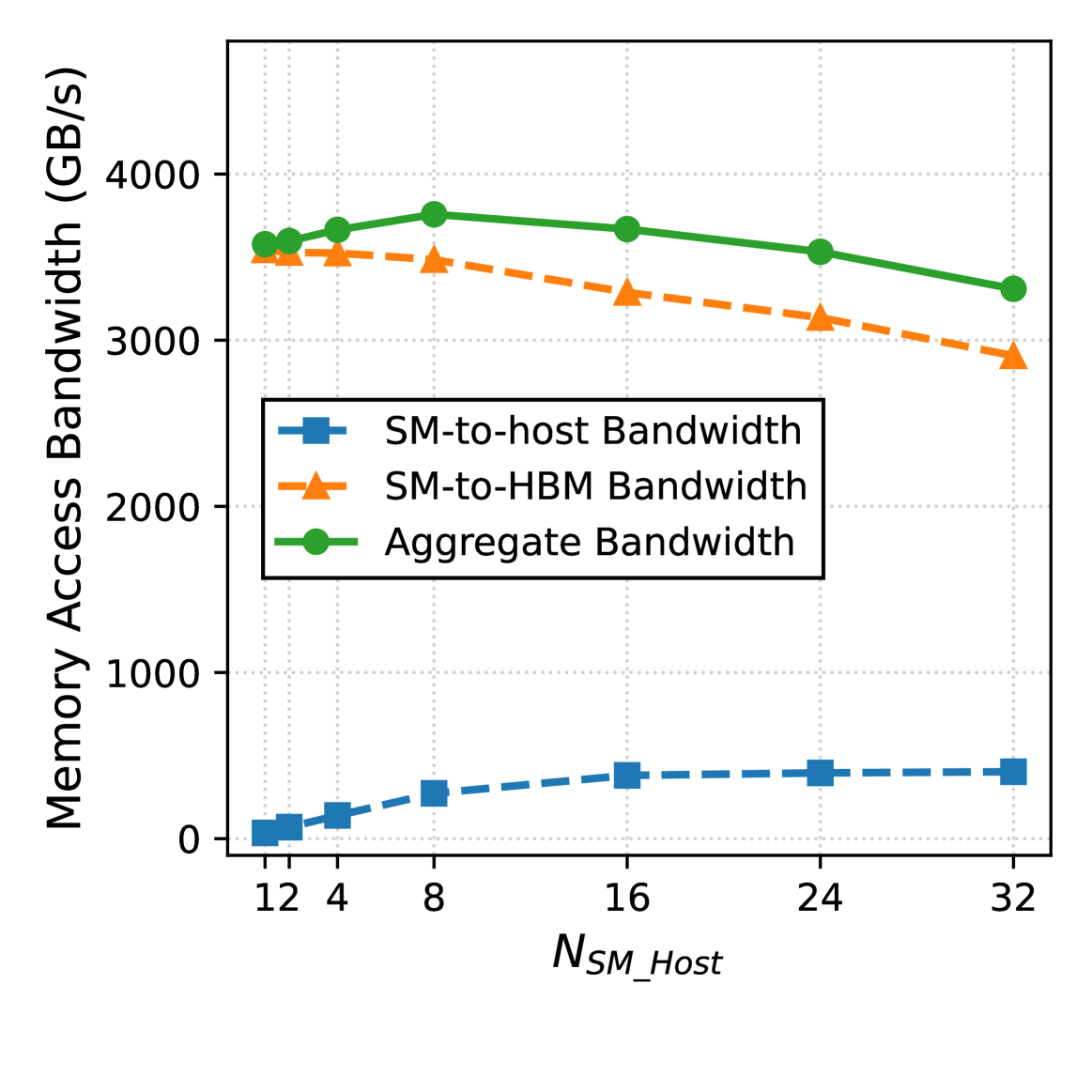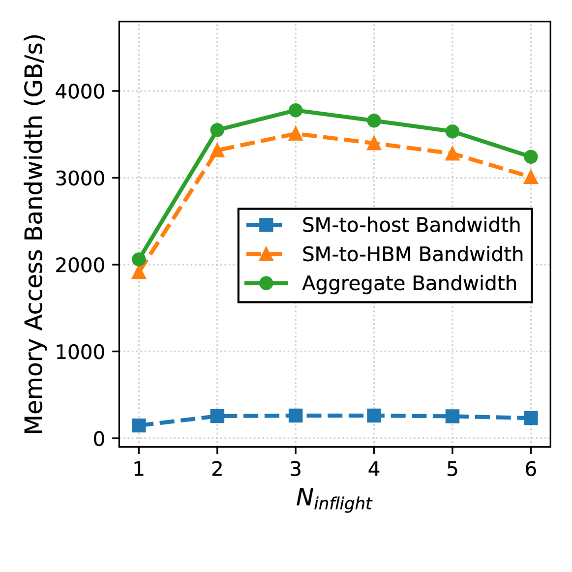The total volume of SM-to-host inflight TMA memory requests can be estimated as $N_SM\_host× N_inflight$ , where $N_SM\_host$ is the number of SMs reading from host memory, and $N_inflight$ is the number of inflight TMA requests issued per SM. Fig. 7 illustrates how unconstrained $N_SM$ or $N_inflight$ causes contention that degrades local HBM throughput on the Grace Hopper Superchip. In the first experiment (7(a)), we dedicate 100 SMs to read from local GPU HBM while varying $N_SM$ reading from remote host memory via NVLink-C2C. As shown in the figure, when $N_SM$ exceeds 8, the SM-to-HBM bandwidth drops significantly, dragging down the system’s total aggregate bandwidth. In the second experiment (7(b)), we fixes the number of SMs reading from both host and GPU, but varies $N_inflight$ issued per SM. The results show that excessive in-flight requests from individual SMs to the host also cause a severe slowdown in aggregate bandwidth. Root Cause Analysis: We observe that this bandwidth degradation does not occur when SMs only access HBM, indicating there is contention between the local and remote data paths. While proprietary GPU interconnect details are undisclosed, we hypothesize this stems from poor resource isolation within the memory hierarchy. Specifically, once the host-GPU interconnect saturates, excess in-flight remote requests cannot drain. These stalled requests accumulate and exhaust shared internal resources (such as L2 cache MSHRs or interconnect routing buffers) which starves the local SM-to-HBM traffic and severely degrades overall performance. Congestion Control Strategy: DAK applies congestion control to remote memory accesses by limiting the ( $N_inflight$ ) and ( $N_SM$ ). To limit $N_inflight$ , DAK uses the concept of a congestion window from traditional computer networking. Each SM fetching from the host is assigned a maximum allowance of in-flight requests that is sized to saturate the SM-to-host memory bandwidth without exceeding it. A given SM’s TMA engine will strictly cap its asynchronous memory requests to this window. Unlike traditional networking protocols that dynamically adjust this window at runtime (which would incur significant runtime overhead for GPU kernels), DAK assigns the congestion window statically. This optimal static window size is calculated via a lightweight parameter-sweeping profiler executed prior to kernel launch. DAK limits $N_SM$ by ensuring we do not over-assign SMs beyond what is necessary. The optimal host $N_SM$ is determined by two factors: 1) interconnect congestion, and 2) how many SMs are needed to process the offloaded data on the host. To find the optimal $N_SM$ , DAK performs an offline parameter sweep—fixing the required local GPU SMs while varying the host SMs—to identify the exact SM allocation to the host that maximizes end-to-end throughput. This ensures the system provisions exactly enough SMs to saturate the computation needs and avoid congestion. | 256 512 1024 | 102.76 MB 205.52 MB 411.04 MB | 1.05 $×$ 2.10 $×$ 4.19 $×$ | | --- | --- | --- | | 2048 | 822.08 MB | 8.39 $×$ | | 4096 | 1.64 GB | 16.78 $×$ | Table 1: Host-GPU memory traffic across varying sizes ( $N$ ). The size of the matrix offloaded to the host is 98 MB. #### 4.3.2 TMA Multicast for Uncacheable Host Access A critical challenge in direct-access offloading is that host-homed memory is uncacheable by the GPU, completely bypassing the L2 cache. Our experiment shows that this architectural limitation applies to both traditional PCIe-connected systems and even coherent CPU-GPU platforms Even on the Grace Hopper Superchip, while the NVLink-C2C supports coherent unified memory, direct host-homed memory accesses bypass the GPU’s L2 cache to maintain hardware coherence without triggering a page migration.. Consequently, direct host access suffers from severe read amplification: if multiple SMs request the same remote tile, the identical data chunk must be transmitted across the host-GPU interconnect multiple times as it cannot cached by GPU L2. For instance, in the scenario depicted in 5(a), output tiles $t_0$ and $t_1$ both require tile row 1 of matrix $A$ , that row is fetched twice over the long-latency interconnect by SM0 and SM1. As shown in Tab. 1, we measured the read amplification effect with different size $N$ in 5(a) and the total host-to-GPU memory transfer scales linearly, reaching 16x more data transfer over CPU-GPU interconnect at $N=4096$ . To eliminate this interconnect bottleneck, DAK uses TMA Multicast and host-aware tile scheduling: - TMA Multicast: DAK leverages the advanced TMA Multicast capabilities [nvidia_cuda_programming_guide_tma]. Instead of each SM issuing independent remote fetches, TMA fetches the host tile across the host-GPU interconnect exactly once. Upon host data arriving at the GPU, the GPU leverages the high-speed intra-cluster Network-on-Chip (NoC) to spatially broadcast the data using Distributed Shared Memory (DSMEM). Physically, the NoC routes the single data payload and simultaneously writes it directly into the SRAM banks of the SMEM for all targeted SMs. - Host-Locality-First Tile Scheduling: Unlike traditional scheduling that optimizes for HBM locality or L2 cache hit rates, DAK implements host-locality-first SM scheduling to enable efficient multicast. Specifically, the producer warps of SMs accessing the same host tile chunk are grouped into the same thread block cluster, which are guaranteed to be co-scheduled simultaneously. Only the producer warp of one SM in the cluster initiates multicast, which reads the tile chunk from host memory once and then stores it to the SMEM slot of all SMs in the cluster. ## 5 Implementation We implemented DAK in approximately 1,300 lines of Python and 2,700 lines of CUDA C++, leveraging CUTLASS to construct our direct-access kernels. The code is open-sourced at https://github.com/shouxulin/DirectAccessKernel.git. Our system is designed for seamless integration into existing deep learning ecosystems and easy portability, with four key aspects: PyTorch Interface: We expose two custom PyTorch modules, SplitK_GEMM and SplitK_FlashAttn, which serve as drop-in replacements for the native nn.Linear and attention layers. This API design allows users to adopt DAK by simply swapping the corresponding layers during initialization, without modifying the model architecture code. Supporting FlashAttention: SplitK_FlashAttn follows the same interface as Pytorch’s Scaled Dot-Product Attention (SDPA) [pytorch_docs_sdpa], while extending it with support for partitioned KV cache access via TMA. It partitions the KV cache along the batch dimension—storing the cache for a subset of requests in local GPU memory and the remainder in remote host memory. Similar to our linear operation kernels, SplitK_FlashAttn supports placing the KV cache into either host memory or HBM based on a given offload ratio. CUDA Graph Optimization: To eliminate CPU-side kernel launch overheads during the latency-sensitive decoding phase, DAK fully supports CUDA Graphs. We pre-allocate the KV cache using PyTorch’s StaticCache, to capture the execution graph using standard APIs, and seamlessly replay it across all subsequent decoding steps. Cross-Architecture Adaptation: To adapt to different GPU generations, we swap the underlying CUTE compute atoms to perform matrix multiplication for that specific architecture (e.g., adapting to different tensor core generations). Furthermore, we expose tunable parameters for the TMA chunk size and maximum in-flight requests. This allows the system to easily calibrate to different SMEM size and interconnect bandwidth limits on different architectures. <details> <summary>2604.26074v1/x10.png Details</summary>  ### Visual Description ## Line Chart: Effective Bandwidth and TPOT vs Offloading Ratio ### Overview The image contains two side-by-side line charts comparing the performance of four computational methods (DAK, FlexGen, vLLM_prefetch, vLLM_uvm) across two metrics: **Effective Bandwidth (GB/s)** and **TPOT (Relative to DAK)** as a function of **Offloading Ratio (%)**. The charts reveal how computational efficiency and relative performance degrade with increasing offloading. --- ### Components/Axes #### Left Chart: Effective Bandwidth (GB/s) - **X-axis**: Offloading ratio (%) ranging from 0% to 100% in 10% increments. - **Y-axis**: Effective Bandwidth (GB/s) from 0 to 3000. - **Legend**: - **DAK**: Orange circles (●) - **FlexGen**: Blue squares (■) - **vLLM_prefetch**: Green triangles (▲) - **vLLM_uvm**: Purple diamonds (◆) #### Right Chart: TPOT (Relative to DAK) - **X-axis**: Offloading ratio (%) identical to the left chart. - **Y-axis**: TPOT (Relative to DAK) from 0 to 2.0. - **Legend**: Same color/marker scheme as the left chart. --- ### Detailed Analysis #### Left Chart: Effective Bandwidth 1. **DAK (● Orange)**: - Starts at ~3000 GB/s at 0% offloading. - Drops sharply to ~500 GB/s at 100% offloading. - Steep decline suggests high sensitivity to offloading. 2. **FlexGen (■ Blue)**: - Begins at ~2000 GB/s at 0%. - Declines gradually to ~300 GB/s at 100%. - Less steep than DAK but still significant loss. 3. **vLLM_prefetch (▲ Green)**: - Starts at ~1000 GB/s at 0%. - Decreases to ~200 GB/s at 100%. - Slower decline than DAK/FlexGen. 4. **vLLM_uvm (◆ Purple)**: - Begins at ~1500 GB/s at 0%. - Drops to ~250 GB/s at 100%. - Intermediate decline rate between FlexGen and vLLM_prefetch. #### Right Chart: TPOT (Relative to DAK) 1. **DAK (● Orange)**: - Flat line at **1.0** across all offloading ratios (baseline). 2. **FlexGen (■ Blue)**: - Starts at ~2.0 TPOT at 0% offloading. - Decreases to ~1.2 TPOT at 100%. - Maintains higher efficiency than DAK. 3. **vLLM_prefetch (▲ Green)**: - Starts at ~1.5 TPOT at 0%. - Declines to ~1.2 TPOT at 100%. - Slightly less efficient than FlexGen. 4. **vLLM_uvm (◆ Purple)**: - Begins at ~1.8 TPOT at 0%. - Drops to ~1.3 TPOT at 100%. - Most efficient relative to DAK at all offloading ratios. --- ### Key Observations 1. **Bandwidth Degradation**: - All methods lose bandwidth as offloading increases, but DAK experiences the steepest decline. - vLLM_uvm retains the highest bandwidth at 100% offloading (~250 GB/s vs. DAK’s ~500 GB/s). 2. **TPOT Efficiency**: - FlexGen and vLLM_uvm consistently outperform DAK, with vLLM_uvm achieving the highest TPOT (~1.8 at 0% offloading). - At 100% offloading, all methods converge to TPOT ~1.2–1.3, indicating similar relative efficiency. 3. **Trade-offs**: - Higher offloading reduces absolute bandwidth but may improve relative efficiency (TPOT). - vLLM_uvm balances bandwidth retention and efficiency better than other methods. --- ### Interpretation The data demonstrates that **offloading reduces computational bandwidth** for all methods, with DAK being the most impacted. However, **vLLM_uvm** emerges as the most efficient approach, maintaining higher TPOT values (relative to DAK) across all offloading ratios. This suggests that vLLM_uvm optimizes resource usage better than DAK or FlexGen, particularly at higher offloading percentages. The convergence of TPOT values at 100% offloading implies diminishing returns in efficiency gains beyond a certain point. These trends highlight the importance of method selection based on workload requirements for bandwidth vs. computational efficiency. </details> (a) OPT-30b on GH200 <details> <summary>2604.26074v1/x11.png Details</summary>  ### Visual Description ## Line Graphs: Effective Bandwidth and TPOT Relative to DAK ### Overview The image contains two side-by-side line graphs. The left graph plots **Effective Bandwidth (GB/s)** against **Offloading ratio (%)**, while the right graph plots **TPOT (Relative to DAK)** against the same x-axis. Both graphs include three data series represented by distinct markers and colors: orange circles, blue squares, and purple diamonds. The legend is positioned on the right side of each graph, but the labels for the series are not explicitly stated in the image. --- ### Components/Axes - **Left Graph (Effective Bandwidth):** - **X-axis**: Offloading ratio (%) ranging from 0 to 100. - **Y-axis**: Effective Bandwidth (GB/s) ranging from 0 to 2500. - **Data Series**: - Orange circles (solid line). - Blue squares (solid line). - Purple diamonds (solid line). - **Legend**: Located on the right side of the graph, with colors matching the data series. - **Right Graph (TPOT Relative to DAK):** - **X-axis**: Offloading ratio (%) ranging from 0 to 100. - **Y-axis**: TPOT (Relative to DAK) ranging from 0 to 4. - **Data Series**: - Orange circles (dashed line). - Blue squares (dashed line). - Purple diamonds (dashed line). - **Legend**: Located on the right side of the graph, with colors matching the data series. --- ### Detailed Analysis #### Left Graph (Effective Bandwidth) 1. **Orange Circles (Solid Line)**: - Starts at ~2400 GB/s at 0% offloading. - Drops sharply to ~500 GB/s at 50% offloading. - Levels off to ~400 GB/s at 100% offloading. 2. **Blue Squares (Solid Line)**: - Remains relatively flat at ~500 GB/s across all offloading ratios. 3. **Purple Diamonds (Solid Line)**: - Starts at ~1400 GB/s at 0% offloading. - Drops to ~300 GB/s at 50% offloading. - Levels off to ~250 GB/s at 100% offloading. #### Right Graph (TPOT Relative to DAK) 1. **Orange Circles (Dashed Line)**: - Remains flat at ~1 across all offloading ratios. 2. **Blue Squares (Dashed Line)**: - Starts at ~4 at 0% offloading. - Drops to ~2 at 50% offloading. - Levels off to ~1.5 at 100% offloading. 3. **Purple Diamonds (Dashed Line)**: - Starts at ~1.5 at 0% offloading. - Peaks at ~2.5 at 50% offloading. - Drops to ~1.2 at 100% offloading. --- ### Key Observations 1. **Left Graph Trends**: - The orange line (Series A) exhibits the steepest decline in effective bandwidth with increasing offloading. - The blue line (Series B) shows minimal change, suggesting stability. - The purple line (Series C) has a moderate decline, followed by stabilization. 2. **Right Graph Trends**: - The blue line (Series B) shows the most significant drop in TPOT relative to DAK. - The orange line (Series A) remains constant, indicating no change in TPOT. - The purple line (Series C) exhibits a non-linear trend, peaking at 50% offloading before declining. --- ### Interpretation - **Effective Bandwidth**: The left graph suggests that higher offloading ratios reduce bandwidth efficiency, with Series A (orange) being the most affected. Series B (blue) remains unaffected, possibly due to inherent stability or design constraints. - **TPOT Relative to DAK**: The right graph indicates that Series B (blue) experiences the greatest reduction in TPOT, while Series C (purple) shows a paradoxical increase at 50% offloading. This could imply that offloading strategies vary in effectiveness across series, with Series C potentially optimizing performance at intermediate offloading ratios. - **Anomalies**: The purple line in the right graph (Series C) deviates from the general trend, suggesting a unique relationship between offloading and TPOT for this series. --- ### Notes on Data Extraction - All values are approximate, with uncertainty due to the absence of explicit numerical labels on the graph. - The legend colors (orange, blue, purple) are cross-referenced with the data series to ensure accuracy. - The spatial positioning of the legend (right side of each graph) and the use of solid/dashed lines for differentiation are consistent across both graphs. </details> (b) OPT-6.7b on GH200 <details> <summary>2604.26074v1/x12.png Details</summary>  ### Visual Description ## Line Charts: Effective Bandwidth and TPOT Relative to DAK ### Overview The image contains two side-by-side line charts analyzing system performance metrics as a function of offloading ratio (%). The left chart measures **Effective Bandwidth (GB/s)**, while the right chart measures **TPOT (Relative to DAK)**. Both charts use offloading ratio (%) as the x-axis, ranging from 0% to 100%. --- ### Components/Axes #### Left Chart: Effective Bandwidth (GB/s) - **Y-axis**: Effective Bandwidth (GB/s), logarithmic scale from 0 to 1250. - **X-axis**: Offloading ratio (%), linear scale from 0% to 100%. - **Legend** (top-left): - Orange circles: Line A - Blue squares: Line B - Green triangles: Line C - Purple diamonds: Line D #### Right Chart: TPOT (Relative to DAK) - **Y-axis**: TPOT (Relative to DAK), linear scale from 0 to 3. - **X-axis**: Offloading ratio (%), linear scale from 0% to 100%. - **Legend** (top-left): - Orange circles: Line A - Blue squares: Line B - Green triangles: Line C - **Note**: Purple diamonds (Line D from left chart) appear in the right chart but are **not listed in the legend**. --- ### Detailed Analysis #### Left Chart: Effective Bandwidth 1. **Line A (Orange Circles)**: - Starts at **1300 GB/s** at 0% offloading. - Drops sharply to **~700 GB/s** at 10% offloading. - Continues declining to **~50 GB/s** at 100% offloading. 2. **Line B (Blue Squares)**: - Starts at **1200 GB/s** at 0% offloading. - Decreases to **~1100 GB/s** at 10% offloading. - Further declines to **~50 GB/s** at 100% offloading. 3. **Line C (Green Triangles)**: - Starts at **1100 GB/s** at 0% offloading. - Drops to **~1000 GB/s** at 10% offloading. - Continues to **~50 GB/s** at 100% offloading. 4. **Line D (Purple Diamonds)**: - Starts at **1200 GB/s** at 0% offloading. - Peaks at **1300 GB/s** at 10% offloading. - Declines to **~50 GB/s** at 100% offloading. #### Right Chart: TPOT Relative to DAK 1. **Line A (Orange Circles)**: - Remains flat at **~1** across all offloading ratios. 2. **Line B (Blue Squares)**: - Starts at **1** at 0% offloading. - Peaks at **2.5** at 10% offloading. - Drops to **1** at 100% offloading. 3. **Line C (Green Triangles)**: - Starts at **1** at 0% offloading. - Peaks at **2** at 10% offloading. - Drops to **1** at 100% offloading. 4. **Line D (Purple Diamonds)**: - Starts at **1** at 0% offloading. - Peaks at **3** at 10% offloading. - Declines to **1.5** at 100% offloading. --- ### Key Observations 1. **Left Chart Trends**: - All lines exhibit a **sharp decline** in effective bandwidth as offloading ratio increases. - Line D (purple diamonds) uniquely **peaks at 10% offloading** before declining, suggesting a temporary performance boost. 2. **Right Chart Trends**: - Lines B, C, and D show **temporary peaks at 10% offloading** (2.5, 2, and 3, respectively), then stabilize. - Line A (orange circles) remains **constant at 1**, indicating no deviation from DAK baseline. 3. **Inconsistency**: - Purple diamonds (Line D) appear in the right chart but are **not included in the legend**, suggesting a potential labeling error. --- ### Interpretation 1. **Performance Trade-offs**: - Increased offloading reduces effective bandwidth across all metrics, but Line D (purple) shows a **non-linear response** with a 10% offloading peak, possibly due to caching or parallelization effects. 2. **TPOT Anomalies**: - The TPOT peaks at 10% offloading for Lines B, C, and D suggest **temporary efficiency gains** relative to DAK, likely due to optimized resource allocation at low offloading ratios. - Line D’s TPOT peak (3x DAK) aligns with its bandwidth peak, indicating a **correlated performance anomaly**. 3. **Legend Discrepancy**: - The absence of Line D (purple diamonds) in the right chart’s legend implies either a **data omission** or a **mislabeling error**, which could mislead interpretation. --- ### Conclusion The charts highlight that offloading ratio significantly impacts bandwidth and TPOT, with Line D (purple) exhibiting unique behavior. The 10% offloading peak in both metrics suggests a critical threshold for performance optimization, warranting further investigation into the underlying mechanisms. The legend inconsistency in the right chart requires clarification to ensure accurate analysis. 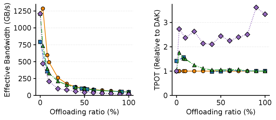</details> (c) OPT-30b on RTX6000 Pro Blackwell <details> <summary>2604.26074v1/x13.png Details</summary>  ### Visual Description ## Line Graphs: Effective Bandwidth and TPOP vs Offloading Ratio ### Overview The image contains two line graphs comparing system performance metrics (Effective Bandwidth and TPOP relative to DAK) across varying offloading ratios (0% to 100%). Each graph uses distinct markers and colors to represent different data series, with trends showing how performance degrades or stabilizes as offloading increases. --- ### Components/Axes #### Left Graph: Effective Bandwidth (GB/s) - **X-axis**: Offloading ratio (%) (0 to 100 in 50% increments) - **Y-axis**: Effective Bandwidth (GB/s) (0 to 1250 in 250 increments) - **Legend**: - Orange Circle - Green Triangle - Blue Square - Purple Diamond #### Right Graph: TPOP (Relative to DAK) - **X-axis**: Offloading ratio (%) (0 to 100 in 50% increments) - **Y-axis**: TPOP (Relative to DAK) (0 to 3 in 1.0 increments) - **Legend**: - Orange Circle - Green Triangle - Purple Diamond --- ### Detailed Analysis #### Left Graph: Effective Bandwidth 1. **Orange Circle** (Highest initial value): - Starts at ~1250 GB/s at 0% offloading. - Drops sharply to ~500 GB/s at 10% offloading. - Plateaus near ~250 GB/s from 20% to 100% offloading. 2. **Green Triangle**: - Begins at ~750 GB/s at 0% offloading. - Declines to ~250 GB/s at 20% offloading. - Stabilizes near ~100 GB/s from 30% to 100% offloading. 3. **Blue Square**: - Starts at ~500 GB/s at 0% offloading. - Decreases to ~100 GB/s at 30% offloading. - Remains flat at ~50 GB/s from 40% to 100% offloading. 4. **Purple Diamond**: - Initiates at ~1000 GB/s at 0% offloading. - Falls to ~200 GB/s at 20% offloading. - Plateaus near ~100 GB/s from 30% to 100% offloading. #### Right Graph: TPOP Relative to DAK 1. **Orange Circle**: - Remains constant at ~1.0 across all offloading ratios. 2. **Green Triangle**: - Starts at ~2.5 at 0% offloading. - Dips to ~1.5 at 10% offloading. - Stabilizes near ~1.0 from 20% to 100% offloading. 3. **Purple Diamond**: - Begins at ~1.0 at 0% offloading. - Rises to ~3.0 at 50% offloading. - Fluctuates between ~2.0 and ~3.0 from 60% to 100% offloading. --- ### Key Observations 1. **Left Graph**: - All data series show significant bandwidth degradation with increasing offloading. - Orange Circle and Purple Diamond experience the steepest initial declines. - Blue Square stabilizes at the lowest bandwidth (~50 GB/s) at high offloading ratios. 2. **Right Graph**: - Orange Circle (stable TPOP) suggests minimal impact on DAK efficiency. - Purple Diamond exhibits the most variability, with a sharp rise at 50% offloading. - Green Triangle shows a notable dip at 10% offloading, then stabilizes. --- ### Interpretation - **Bandwidth Degradation**: Higher offloading ratios correlate with reduced effective bandwidth, but the rate of decline varies by data series. The Orange Circle and Purple Diamond lines suggest these configurations are more sensitive to offloading. - **TPOP Stability**: The Orange Circle’s consistent TPOP (~1.0) implies it maintains DAK efficiency regardless of offloading. In contrast, the Purple Diamond’s fluctuating TPOP indicates variable DAK performance under high offloading. - **Anomalies**: The Green Triangle’s sharp dip at 10% offloading in the left graph and subsequent stabilization in the right graph may reflect a threshold effect, where offloading beyond 10% no longer significantly impacts bandwidth or TPOP. This analysis highlights trade-offs between offloading and system performance, with specific configurations (e.g., Orange Circle) offering stability in TPOP despite bandwidth reductions. </details> (d) OPT-6.7b and on RTX6000 Pro Blackwell Figure 8: Performance w/ batch size = 8 under vary offloading ratios. ## 6 Evaluation We evaluate DAK by answering the following questions: (1) How does DAK compare to baselines across various offloading ratios, hardware architectures, and models? (2) Can DAK enable large models to run efficiently when their memory footprints exceed GPU capacity (§ 6.1)? (3) What is the performance gain of the greedy offloading algorithm? (4) How effective are the TMA optimizations (§ 6.2)? Testbed & Workloads: We evaluate our system across two distinct NVIDIA GPU architectures to capture a range of interconnect technologies and GPU generations: - Grace Hopper (GH200): An NVLink-C2C-based system featuring a 900 GB/s host-GPU interconnect and 480 GB of host memory. The GPU includes 96 GB of local HBM3 with 4.0 TB/s of bandwidth. - RTX 6000 Pro Blackwell: A PCIe Gen5-based system with a unidirectional host-GPU bandwidth of 64 GB/s and 512 GB of host memory. The GPU features 96 GB of local GDDR7 with 1.8 TB/s of bandwidth. Our experiments are conducted under an offline, batched-inference setup. We evaluate a diverse set of LLMs across varying batch sizes and prompt lengths, decoding 32 tokens per request. Unless otherwise specified, the prompt length is set to 32. We test across multiple models (OPT-30b, OPT-6.7b, and Llama-2-7b). In our evaluation, we compare our system against three baselines: FlexGen [sheng2023flexgen], a state-of-the-art offloading framework that uses double-buffered, layer-by-layer prefetching to manage weights and KV caches across tiered memory; vLLM-prefetch [dao2022flashattention], a config of vLLM that implements asynchronous prefetch of KV blocks and weights from host memory to GPU HBM; and vLLM-uvm, a vLLM variant that utilizes NVIDIA Unified Virtual Memory (UVM), which relies on hardware page faults and system managed paging migrations to access host memory. ### 6.1 DAK End-to-End Performance In this experiment, we compare DAK’s performance against baseline systems by sweeping the offloading ratio from 0% to 100% for the OPT-30B and OPT-6.7B models. We evaluate using two primary metrics: (1) Time Per Output Token (TPOT), representing the end-to-end decoding latency for a single token, and (2) Effective Bandwidth ( $EB$ ) defined as the total model size divided by TPOT, which shows the achieved aggregated memory bandwidth. Weights Offload: We first measure performance using a batch size of 8. In this experiment, because the batch size is small, the memory footprint of the KV cache is also small, meaning the offloaded memory is primarily model weights. With a small batch size, the decoding is mostly memory-bound. As shown in Fig. 8, DAK consistently achieves the highest $EB$ across all models and offload ratios. On the GH200 system, DAK’s direct-access approach provides massive advantages across all offload ratios, yielding 1.5 $×$ to 5 $×$ performance gains. DAK also achieves optimal aggregate system memory bandwidth through offloading. For instance, with OPT-30B at a 10% offload ratio, DAK sustains 3,300 GB/s, achieving a near-optimal aggregate memory bandwidth that approaches the theoretical peak of NVLink-C2C + HBM. In contrast, prefetching baselines suffer bandwidth degradation across all offload ratios. DAK’s high memory bandwidth also translates directly into a lower TPOT. As a note, in 11(b), FlexGen exhibits low performance on OPT-6.7B because kernel launch overhead dominates for smaller models, whereas vLLM and DAK utilize CUDA Graphs to mitigate this overhead entirely. As shown in 8(c) and 8(d), on the PCIe-based RTX 6000 Blackwell system, DAK remains strictly better to all prefetching schemes. It achieves near-ideal aggregate system memory bandwidth, demonstrating a 4% improvement through offloading that closely approaches the theoretical limits of the PCIe Gen5 interconnect. At low-to-medium offload ratios (0%–40%), DAK delivers a 1.3 $×$ to 3 $×$ improvement in both $EB$ and TPOT compared to vLLM-prefetch and FlexGen. Beyond a 40% offload ratio, the performance of DAK, vLLM-prefetch, and FlexGen converges, as operation latency becomes entirely bottlenecked by the physical limits of transferring weights over the low-bandwidth PCIe link. The vLLM-UVM baseline performs significantly worse than all other systems due to the severe latency penalties of page-fault and paging migration overheads over PCIe. 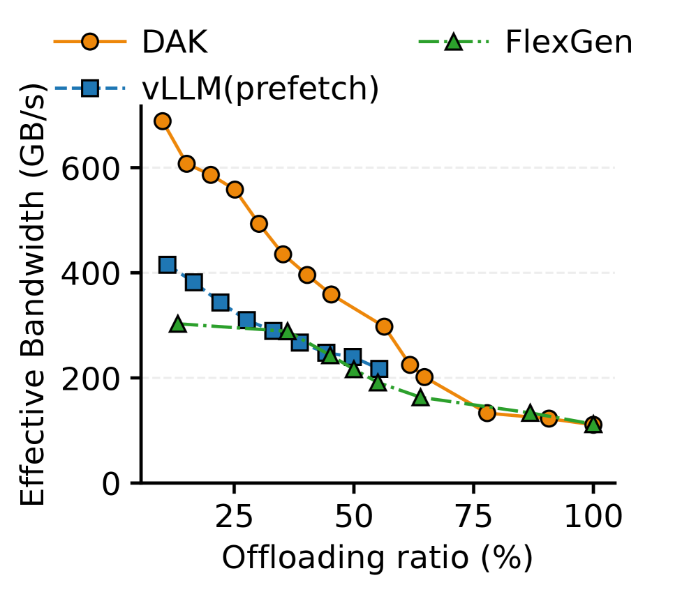<details> <summary>2604.26074v1/x14.png Details</summary>  ### Visual Description ## Line Graph: Effective Bandwidth vs. Offloading Ratio ### Overview The graph compares the effective bandwidth (GB/s) of three technologies—DAK, FlexGen, and vLLM (prefetch)—across varying offloading ratios (0% to 100%). All three show a downward trend in bandwidth as offloading increases, but with distinct performance characteristics. ### Components/Axes - **X-axis**: Offloading ratio (%) [0, 25, 50, 75, 100] - **Y-axis**: Effective Bandwidth (GB/s) [0, 200, 400, 600] - **Legend**: - **DAK**: Orange circles (solid line) - **FlexGen**: Green triangles (dashed line) - **vLLM (prefetch)**: Blue squares (dotted line) ### Detailed Analysis 1. **DAK (Orange Circles)**: - Starts at ~650 GB/s at 0% offloading. - Declines steadily, reaching ~100 GB/s at 100% offloading. - Key points: - 25%: ~550 GB/s - 50%: ~300 GB/s - 75%: ~150 GB/s 2. **FlexGen (Green Triangles)**: - Begins at ~300 GB/s at 0% offloading. - Declines gradually, ending near ~100 GB/s at 100% offloading. - Key points: - 25%: ~280 GB/s - 50%: ~200 GB/s - 75%: ~120 GB/s 3. **vLLM (Prefetch) (Blue Squares)**: - Starts at ~400 GB/s at 0% offloading. - Sharp decline after 25% offloading, dropping to ~100 GB/s by 100%. - Key points: - 25%: ~380 GB/s - 50%: ~220 GB/s - 75%: ~110 GB/s ### Key Observations - **DAK** maintains the highest bandwidth across all offloading ratios, suggesting superior scalability. - **vLLM (prefetch)** experiences the steepest drop, particularly between 25% and 50% offloading, indicating potential inefficiencies in prefetching at higher ratios. - **FlexGen** exhibits a moderate decline, balancing performance and scalability. ### Interpretation The data suggests that **DAK** is the most robust technology for maintaining effective bandwidth as offloading increases, likely due to optimized resource allocation or architecture. **vLLM (prefetch)**’s sharp decline implies that prefetching mechanisms may become a bottleneck at higher offloading ratios, possibly due to overhead or contention. **FlexGen** offers a middle-ground solution, with a slower degradation rate than vLLM but lower baseline performance than DAK. The trends highlight trade-offs between offloading efficiency and bandwidth retention, with DAK emerging as the most scalable option for high offloading scenarios. 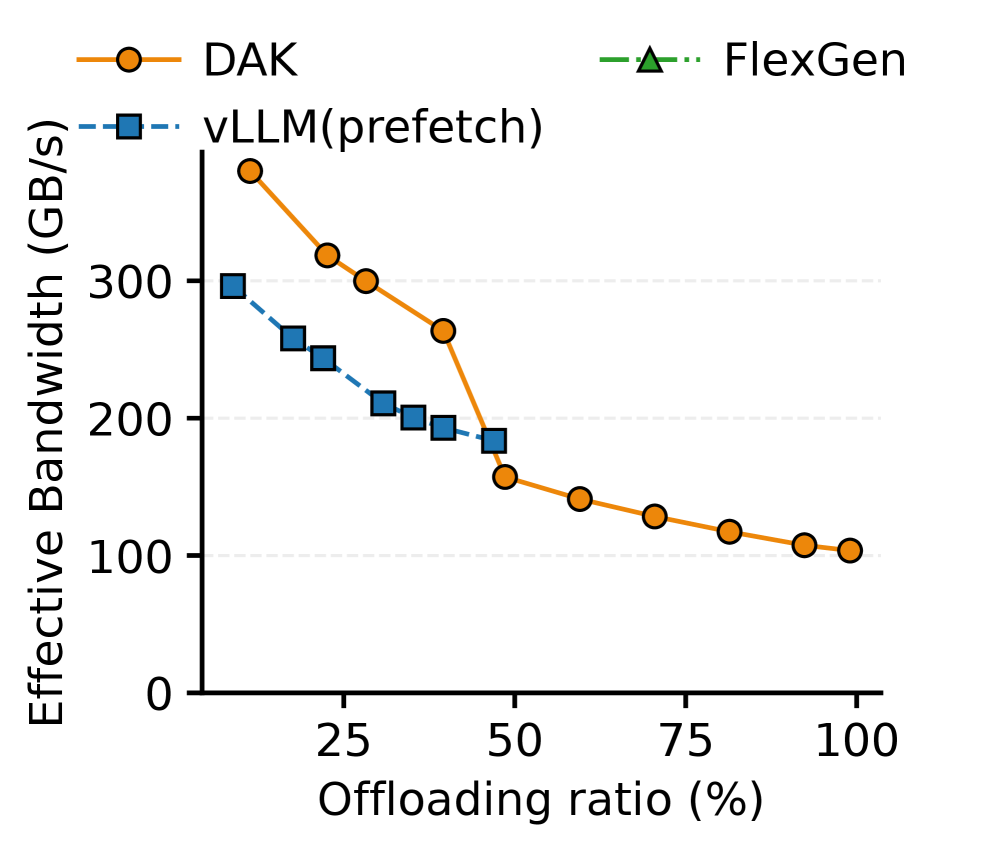</details> (a) OPT-30b on GH200 <details> <summary>2604.26074v1/x15.png Details</summary>  ### Visual Description ## Line Graph: Effective Bandwidth vs. Offloading Ratio ### Overview The image is a line graph comparing three data series: **DAK**, **vLLM (prefetch)**, and **FlexGen**, plotted against **offloading ratio (%)** on the x-axis and **effective bandwidth (GB/s)** on the y-axis. The graph shows how effective bandwidth decreases as offloading ratio increases, with distinct trends for each method. --- ### Components/Axes - **X-axis**: Offloading ratio (%) (0 to 100% in increments of ~25%). - **Y-axis**: Effective Bandwidth (GB/s) (0 to 350 in increments of ~100). - **Legend**: - **DAK**: Orange line with solid circles (top-right placement). - **vLLM (prefetch)**: Dashed blue line with squares. - **FlexGen**: Dotted green line with triangles (only appears at 100% offloading). --- ### Detailed Analysis #### DAK (Orange Line) - **Trend**: Steady decline from ~350 GB/s at 0% offloading to ~100 GB/s at 100% offloading. - **Key Points**: - 0%: ~350 GB/s. - 25%: ~310 GB/s. - 50%: ~180 GB/s. - 75%: ~120 GB/s. - 100%: ~100 GB/s. #### vLLM (Prefetch) (Blue Dashed Line) - **Trend**: Sharp decline, with a steeper drop after 50% offloading. - **Key Points**: - 0%: ~300 GB/s. - 25%: ~240 GB/s. - 50%: ~200 GB/s. - 75%: ~50 GB/s (estimated from graph curvature). - 100%: ~50 GB/s (data point overlaps FlexGen at 100%). #### FlexGen (Green Dotted Line) - **Trend**: Only visible at 100% offloading, with a single data point. - **Key Point**: - 100%: ~5 GB/s (data point labeled with green triangle). --- ### Key Observations 1. **DAK** maintains the highest effective bandwidth across all offloading ratios but shows gradual degradation. 2. **vLLM (prefetch)** experiences a **nonlinear drop**, with bandwidth plummeting to ~50 GB/s at 75% and 100% offloading. 3. **FlexGen** is only plotted at 100% offloading, where it achieves ~5 GB/s, significantly lower than other methods at the same ratio. 4. **vLLM** and **FlexGen** converge at 100% offloading (~50 GB/s for vLLM vs. ~5 GB/s for FlexGen), suggesting a potential anomaly or missing data for FlexGen at lower ratios. --- ### Interpretation - **DAK** demonstrates **consistent scalability**, retaining ~70% of its initial bandwidth at 50% offloading, indicating robust performance under partial offloading. - **vLLM (prefetch)** exhibits **diminishing returns**, with bandwidth collapsing sharply beyond 50% offloading, suggesting prefetching becomes inefficient at higher ratios. - **FlexGen**’s isolated data point at 100% offloading raises questions: - Is it designed for **full offloading only**? - Why does its bandwidth (~5 GB/s) lag far behind vLLM’s ~50 GB/s at the same ratio? This could imply architectural limitations or a focus on latency over bandwidth. - The **absence of FlexGen data at lower ratios** implies it may not be optimized for partial offloading, unlike DAK and vLLM. --- ### Notable Anomalies - **vLLM vs. FlexGen at 100%**: The ~50 GB/s vs. ~5 GB/s disparity suggests either: - FlexGen prioritizes other metrics (e.g., latency, energy efficiency). - FlexGen’s implementation is incomplete or context-specific. - **DAK’s smooth decline** contrasts with **vLLM’s abrupt drop**, highlighting differences in offloading strategies (e.g., prefetching vs. direct offloading). --- ### Conclusion The graph illustrates trade-offs between offloading ratio and bandwidth efficiency. **DAK** balances scalability and performance, while **vLLM** struggles with high offloading ratios. **FlexGen**’s single data point hints at a specialized use case, but its performance at 100% offloading warrants further investigation. </details> (b) Llama-2-7b on GH200 Figure 9: Performance w/ batch size = 512 under vary offloading ratios KV Cache Offload: We next evaluate performance using a larger batch size of 512. At this scale, the KV cache footprint increases to 45 GB, requiring the system to concurrently manage the offloading of both weights and KV caches. Furthermore, the decoding phase becomes a heterogeneous mix of compute-bound operations (linear layers) and memory-bound operations (attention). Fig. 9 shows that DAK improves up to 2.1x performance compared to baselines on the GH200 system under OPT, and Llama model. DAK achieves this performance for two key reasons: (1) its direct-access paradigm fully utilizes aggregate system bandwidth to accelerate memory-bound attention operations, (2) its offloading algorithm analytically determines the optimal, operation-specific offloading ratios for both weights and KV caches. In contrast, baseline systems apply a naive, uniform offloading strategy that ignores these distinct operation characteristics, and (3) DAK can efficiently handle the read amplification problem with TMA-multicast under large batch sizes. Note that vLLM data points are omitted for offload ratios exceeding 50%, as this is the threshold where vLLM begins offloading the KV cache to CPU memory. In these cases, vLLM falls back to splitting the workload into multiple sub-batches and interleaving the prefill and decode phases, which prevents a clean, isolated measurement of the decode latency for the entire batch. Additionally, FlexGen results for Llama are missing because it is not supported by FlexGen. 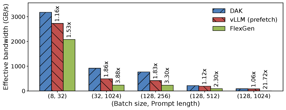<details> <summary>2604.26074v1/x16.png Details</summary>  ### Visual Description ## Bar Chart: Effective Bandwidth Comparison Across Configurations ### Overview The chart compares effective bandwidth (GB/s) of three technologies (DAK, vLLM (prefetch), FlexGen) across five configurations defined by batch size and prompt length pairs. Each bar includes a multiplier indicating performance relative to a baseline. ### Components/Axes - **X-axis**: Configuration pairs (Batch size, Prompt length): (8, 32), (32, 1024), (128, 256), (128, 512), (128, 1024) - **Y-axis**: Effective bandwidth (GB/s), scaled from 0 to 3000. - **Legend**: - Blue (DAK) - Red (vLLM (prefetch)) - Green (FlexGen) ### Detailed Analysis 1. **(8, 32)**: - DAK: ~3100 GB/s (1.16x) - vLLM: ~2700 GB/s (1.53x) - FlexGen: ~2000 GB/s (1.53x) 2. **(32, 1024)**: - DAK: ~900 GB/s (1.86x) - vLLM: ~500 GB/s (3.88x) - FlexGen: ~300 GB/s (3.88x) 3. **(128, 256)**: - DAK: ~700 GB/s (1.83x) - vLLM: ~400 GB/s (3.30x) - FlexGen: ~200 GB/s (3.30x) 4. **(128, 512)**: - DAK: ~200 GB/s (1.12x) - vLLM: ~150 GB/s (2.30x) - FlexGen: ~100 GB/s (2.30x) 5. **(128, 1024)**: - DAK: ~100 GB/s (1.06x) - vLLM: ~80 GB/s (1.72x) - FlexGen: ~50 GB/s (21.72x) ### Key Observations - **DAK** consistently achieves the highest absolute bandwidth, especially in smaller configurations (e.g., 3100 GB/s for (8,32)). - **vLLM** and **FlexGen** show higher multipliers in larger configurations, suggesting better relative efficiency gains compared to DAK. - **FlexGen** exhibits an anomalous 21.72x multiplier in the (128,1024) configuration, far exceeding other values. - Bandwidth decreases as batch size and prompt length increase, but multipliers vary non-linearly. ### Interpretation The data suggests **DAK** is optimized for high-throughput scenarios with smaller batch/prompt sizes, while **vLLM** and **FlexGen** demonstrate superior scaling efficiency in larger configurations. The FlexGen anomaly (21.72x) may indicate a specialized optimization or data anomaly. The trend of decreasing absolute bandwidth with larger configurations aligns with typical memory-bound workloads, but the multiplier discrepancies highlight differing architectural efficiencies. Further investigation into FlexGen’s (128,1024) performance is warranted to validate the outlier. </details> | 8 32 128 | 32 1024 256 | 55.6 GB 55.6 GB 55.6 GB | 0.7 GB 46.51 GB 50.73 GB | 0% 6% 10% | | --- | --- | --- | --- | --- | | 128 | 512 | 55.6 GB | 95.83 GB | 37% | | 128 | 1024 | 55.6 GB | 186.03 GB | 60% | Figure 10: Figure shows the performance for GH200 under different configurations. The table shows the memory footprint for different configurations and the corresponding global memory offload ratio. Optimal Model Offloading: Now, rather than manually sweeping offload ratios, we evaluate DAK’s capability to efficiently run large models on GPUs with limited memory capacity, with the global offloading ratio determined by the real available GPU memory. As shown in Fig. 10, we vary the batch size and prompt length for OPT-30B. Large batch sizes and extended prompt lengths increase the total memory footprint well beyond the available GPU HBM, which dynamically dictates the required global offload ratio. We compare the maximum achievable performance across these configurations against vLLM and FlexGen. DAK consistently outperforms all baselines across every configuration, achieving 1.06 $×$ to 1.83 $×$ speedups over vLLM, and 1.53 $×$ to 21 $×$ speedups over FlexGen. These significant gains highlight the combined effectiveness of DAK’s optimal offloading algorithm and highly efficient direct-access. In Appendix B, we show additional results on OPT-6.7B. 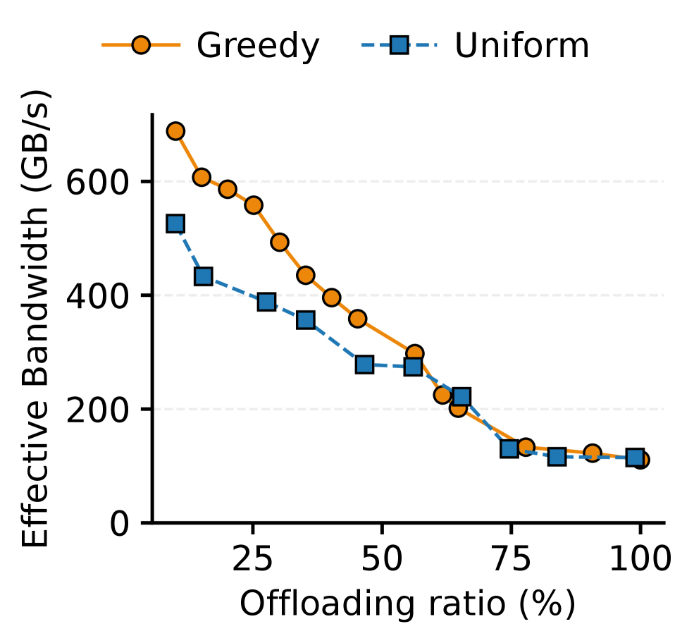<details> <summary>2604.26074v1/x17.png Details</summary>  ### Visual Description ## Line Graph: Effective Bandwidth vs. Offloading Ratio ### Overview The image depicts a line graph comparing the effective bandwidth (GB/s) of two strategies—Greedy and Uniform—as a function of offloading ratio (%). The graph shows two data series with distinct trends, plotted against a Cartesian coordinate system. --- ### Components/Axes - **X-axis (Horizontal)**: - Label: "Offloading ratio (%)" - Scale: 0% to 100% in increments of 25%. - **Y-axis (Vertical)**: - Label: "Effective Bandwidth (GB/s)" - Scale: 0 to 600 GB/s in increments of 200 GB/s. - **Legend**: - Position: Top-right corner. - Entries: - "Greedy" (orange solid circles). - "Uniform" (blue dashed squares). --- ### Detailed Analysis #### Greedy Strategy (Orange Line) - **Trend**: Starts at approximately **650 GB/s** at 0% offloading, decreasing non-linearly to ~100 GB/s at 100% offloading. - **Key Data Points**: - 0%: ~650 GB/s - 25%: ~580 GB/s - 50%: ~350 GB/s - 75%: ~150 GB/s - 100%: ~100 GB/s #### Uniform Strategy (Blue Dashed Line) - **Trend**: Begins at ~500 GB/s at 0% offloading, declining gradually to ~120 GB/s at 100% offloading. - **Key Data Points**: - 0%: ~500 GB/s - 25%: ~400 GB/s - 50%: ~280 GB/s - 75%: ~140 GB/s - 100%: ~120 GB/s --- ### Key Observations 1. **Initial Disparity**: The Greedy strategy outperforms Uniform at lower offloading ratios (e.g., 650 vs. 500 GB/s at 0%). 2. **Convergence**: Both strategies converge near 100% offloading (~100–120 GB/s), suggesting diminishing returns at high offloading. 3. **Rate of Decline**: Greedy’s bandwidth drops more sharply initially (e.g., 650 → 580 GB/s between 0–25%), while Uniform’s decline is more gradual. --- ### Interpretation - **Strategy Implications**: - The Greedy approach is more effective for low-to-moderate offloading (0–50%), but its performance degrades rapidly as offloading increases. - The Uniform strategy maintains steadier performance across all offloading ratios, making it more reliable for high offloading scenarios. - **Underlying Dynamics**: - The divergence at lower offloading ratios may reflect Greedy’s aggressive resource allocation, which becomes unsustainable at higher offloading. - The convergence at 100% offloading implies both strategies face similar bandwidth constraints when fully offloaded. - **Anomalies**: - No outliers detected; both trends follow smooth, predictable declines. --- ### Final Notes The graph highlights a trade-off between initial performance and scalability. Greedy excels in low offloading scenarios but falters under heavy load, while Uniform offers consistent, albeit lower, performance across all conditions. This suggests context-dependent strategy selection based on expected offloading ratios. 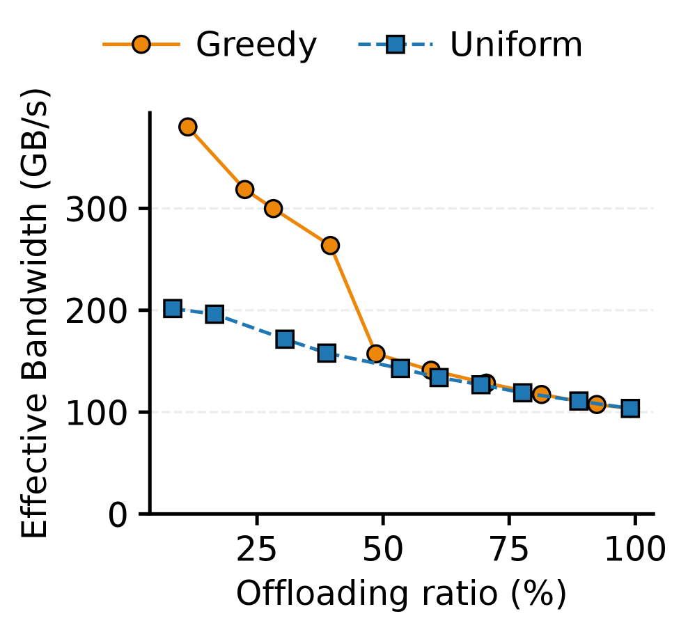</details> (a) OPT-30b on GH200 <details> <summary>2604.26074v1/x18.png Details</summary>  ### Visual Description ## Line Graph: Effective Bandwidth vs Offloading Ratio ### Overview The graph compares two strategies ("Greedy" and "Uniform") for effective bandwidth (GB/s) across varying offloading ratios (0% to 100%). The "Greedy" strategy (orange line with circles) starts with significantly higher bandwidth but declines sharply, while the "Uniform" strategy (blue dashed line with squares) maintains a steadier decline. ### Components/Axes - **X-axis**: Offloading ratio (%) with markers at 0%, 25%, 50%, 75%, and 100%. - **Y-axis**: Effective Bandwidth (GB/s) with markers at 0, 100, 200, and 300 GB/s. - **Legend**: Located at the top-right corner. Orange circles represent "Greedy," and blue squares represent "Uniform." ### Detailed Analysis 1. **Greedy Strategy**: - At 0% offloading: ~350 GB/s (highest point). - At 25% offloading: ~300 GB/s. - At 50% offloading: ~150 GB/s. - At 75% offloading: ~120 GB/s. - At 100% offloading: ~100 GB/s. - **Trend**: Steep decline from 0% to 50%, then gradual decline. 2. **Uniform Strategy**: - At 0% offloading: ~200 GB/s. - At 25% offloading: ~180 GB/s. - At 50% offloading: ~150 GB/s. - At 75% offloading: ~120 GB/s. - At 100% offloading: ~100 GB/s. - **Trend**: Steady linear decline across all offloading ratios. ### Key Observations - The "Greedy" strategy outperforms "Uniform" at low offloading ratios (0–50%) but converges with "Uniform" beyond 50%. - Both strategies plateau near 100 GB/s at 100% offloading. - The "Greedy" line exhibits a nonlinear drop, while "Uniform" follows a consistent linear trend. ### Interpretation The data suggests that the "Greedy" strategy is more effective for low offloading ratios but becomes inefficient as offloading increases. In contrast, the "Uniform" strategy provides stable performance across all ratios but never exceeds the initial bandwidth of "Greedy." The convergence at 50% offloading implies a critical threshold where both strategies yield similar results. This could inform decision-making in resource allocation, favoring "Greedy" for minimal offloading and "Uniform" for higher or variable offloading scenarios. </details> (b) Llama-2-7b on GH200 Figure 11: Compare greedy with uniform offloading. Batch size is 512. 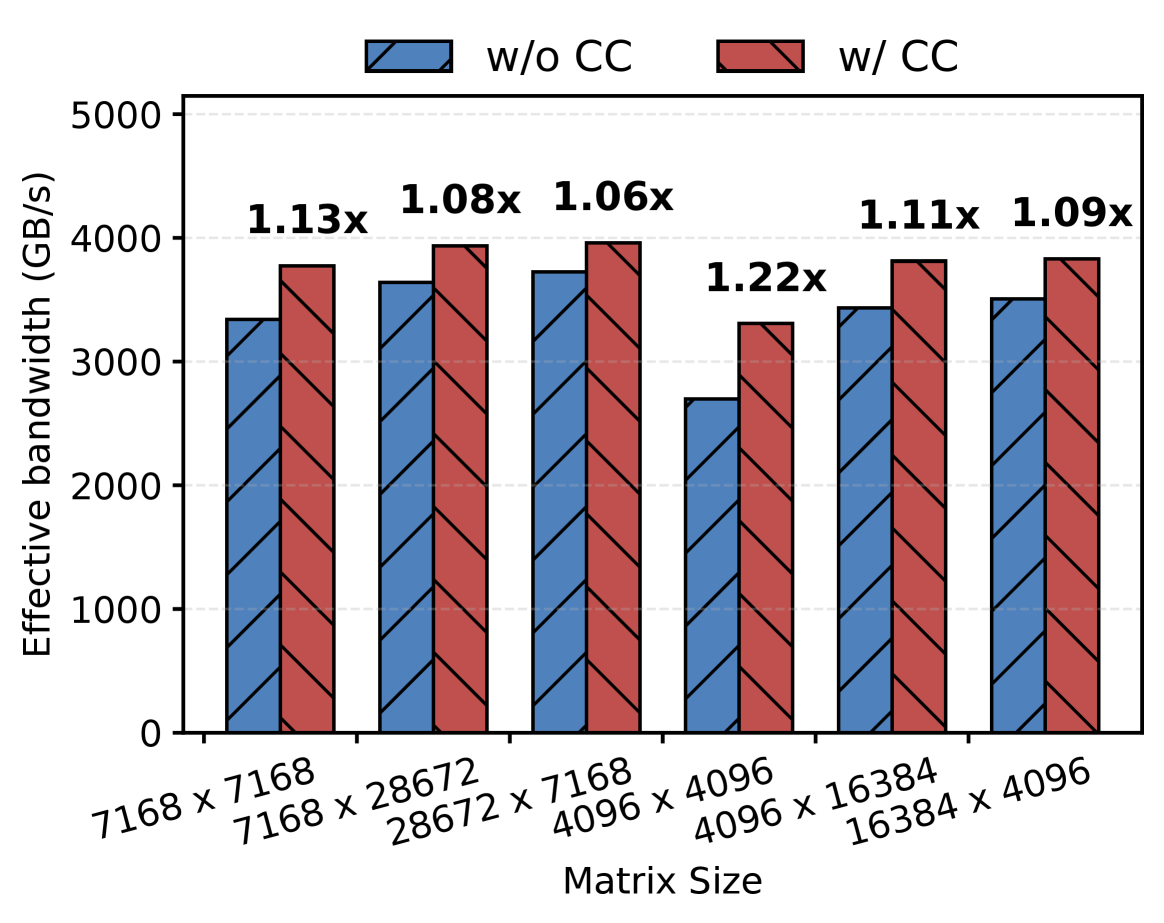<details> <summary>2604.26074v1/x19.png Details</summary>  ### Visual Description ## Bar Chart: Effective Bandwidth Comparison with/without CC ### Overview The chart compares the effective bandwidth (in GB/s) of matrix operations with and without a compression/optimization technique labeled "CC" across six different matrix sizes. Each matrix size has two bars: blue (w/o CC) and red (w/ CC), with performance gains (multipliers) annotated on the red bars. ### Components/Axes - **X-axis (Matrix Size)**: - 7168 x 7168 - 28672 x 28672 - 7168 x 28672 - 4096 x 4096 - 16384 x 4096 - 4096 x 4096 (duplicate entry) - **Y-axis (Effective Bandwidth)**: 0–5000 GB/s, with increments of 1000. - **Legend**: - Blue (w/o CC) - Red (w/ CC) - **Annotations**: Multipliers (e.g., 1.13x) on red bars. ### Detailed Analysis 1. **7168 x 7168**: - w/o CC: ~3300 GB/s - w/ CC: ~3700 GB/s (1.13x gain) 2. **28672 x 28672**: - w/o CC: ~3700 GB/s - w/ CC: ~4000 GB/s (1.08x gain) 3. **7168 x 28672**: - w/o CC: ~3700 GB/s - w/ CC: ~4000 GB/s (1.06x gain) 4. **4096 x 4096**: - w/o CC: ~2700 GB/s - w/ CC: ~3300 GB/s (1.22x gain) 5. **16384 x 4096**: - w/o CC: ~3400 GB/s - w/ CC: ~3800 GB/s (1.11x gain) 6. **4096 x 4096 (duplicate)**: - w/o CC: ~2700 GB/s - w/ CC: ~3300 GB/s (1.09x gain) ### Key Observations - **Performance Gains**: The highest gain (1.22x) occurs for the 4096 x 4096 matrix, while the largest matrices (28672 x 28672 and 7168 x 28672) show the lowest gains (1.08x and 1.06x). - **Trends**: - Smaller matrices (e.g., 4096 x 4096) benefit more from CC. - Larger matrices exhibit diminishing returns. - Rectangular matrices (e.g., 7168 x 28672, 16384 x 4096) show intermediate gains. - **Anomalies**: The duplicate 4096 x 4096 entry with a 1.09x gain (vs. 1.22x for the same size) may indicate a data inconsistency or experimental variation. ### Interpretation The data suggests that the CC technique significantly improves bandwidth efficiency for smaller matrices (e.g., 4096 x 4096), likely due to optimized memory access or algorithmic adjustments at that scale. Larger matrices (e.g., 28672 x 28672) show minimal gains, implying that CC’s effectiveness diminishes with increased problem size, possibly due to memory bandwidth saturation or algorithmic overhead. The rectangular matrices (e.g., 16384 x 4096) demonstrate moderate improvements, highlighting that aspect ratios may influence CC’s impact. These findings could guide optimization strategies for computational workloads, prioritizing CC for smaller or specific matrix dimensions. 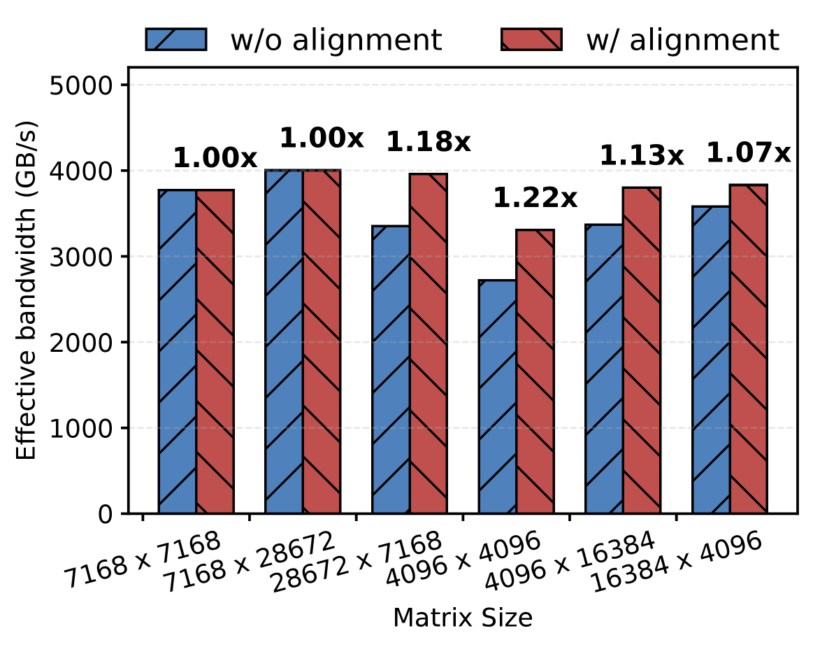</details> (a) Congestion Control Effect <details> <summary>2604.26074v1/x20.png Details</summary>  ### Visual Description ## Bar Chart: Effective Bandwidth Comparison with/without Alignment ### Overview The chart compares the effective bandwidth (in GB/s) of matrix operations with and without alignment across different matrix sizes. Two bars are shown per matrix size: blue for "w/o alignment" and red for "w/ alignment". Each bar includes a multiplier (e.g., 1.00x, 1.18x) indicating the performance improvement relative to the baseline (w/o alignment). ### Components/Axes - **X-axis (Matrix Size)**: - Categories: - 7168 x 7168 - 7168 x 28672 - 28672 x 7168 - 28672 x 4096 - 4096 x 7168 - 4096 x 16384 - 16384 x 4096 - **Y-axis (Effective Bandwidth)**: - Scale: 0 to 5000 GB/s (with gridlines at 1000, 2000, 3000, 4000, 5000). - **Legend**: - Position: Top of the chart. - Labels: - Blue: "w/o alignment" - Red: "w/ alignment" ### Detailed Analysis - **Matrix Size: 7168 x 7168** - w/o alignment: ~3800 GB/s (1.00x) - w/ alignment: ~3800 GB/s (1.00x) - **Matrix Size: 7168 x 28672** - w/o alignment: ~4000 GB/s (1.00x) - w/ alignment: ~4000 GB/s (1.00x) - **Matrix Size: 28672 x 7168** - w/o alignment: ~3400 GB/s (1.18x) - w/ alignment: ~4000 GB/s (1.18x) - **Matrix Size: 28672 x 4096** - w/o alignment: ~2700 GB/s (1.22x) - w/ alignment: ~3300 GB/s (1.22x) - **Matrix Size: 4096 x 7168** - w/o alignment: ~3400 GB/s (1.13x) - w/ alignment: ~3800 GB/s (1.13x) - **Matrix Size: 4096 x 16384** - w/o alignment: ~3400 GB/s (1.07x) - w/ alignment: ~3800 GB/s (1.07x) - **Matrix Size: 16384 x 4096** - w/o alignment: ~3600 GB/s (1.07x) - w/ alignment: ~3900 GB/s (1.07x) ### Key Observations 1. **Alignment Improves Bandwidth**: For all matrix sizes, the "w/ alignment" bars (red) consistently show higher effective bandwidth than "w/o alignment" (blue), with multipliers ranging from 1.00x to 1.22x. 2. **Largest Matrix Size (4096 x 4096)**: Achieves the highest improvement (1.22x), suggesting alignment is most impactful for larger matrices. 3. **Smallest Matrix Size (7168 x 7168)**: No improvement (1.00x), indicating alignment may not benefit smaller matrices. 4. **Asymmetry in Multipliers**: Some matrix sizes (e.g., 28672 x 7168) show higher multipliers than their symmetric counterparts (e.g., 7168 x 28672), possibly due to directional alignment effects. ### Interpretation The data demonstrates that alignment significantly enhances effective bandwidth, particularly for larger matrix operations. The 1.22x improvement at 4096 x 4096 highlights the scalability benefits of alignment. However, the lack of improvement for 7168 x 7168 suggests alignment may not be necessary or effective for smaller matrices. The asymmetry in multipliers (e.g., 28672 x 7168 vs. 7168 x 28672) implies that alignment directionality or implementation specifics might influence performance. This chart underscores the importance of alignment in optimizing computational efficiency for large-scale matrix operations. </details> (b) Kernel Alignment Effect Figure 12: Effectiveness of congestion control and kernel alignment on different matrix sizes. ### 6.2 Effectiveness of DAK Optimizations Next, we run benchmarks on the GH200 system and evaluate DAK’s key design decisions. Greedy Offload Performance: We show that our greedy offload algorithm successfully incorporates the compute- and memory-bound characteristics of individual operations to select the optimal offloading ratio for each. We compare the greedy strategy against a uniform offloading baseline using a batch size of 512, which is a workload that has a mix of compute- and memory-bound operations. As shown in Fig. 11, the greedy algorithm outperforms uniform offloading by 1.5 $×$ when the offloading ratio is below 60%. This is because the greedy approach identifies the turning point of each kernel’s $EB$ and prioritizes offloading compute-bound kernels, which are significantly less sensitive to remote memory access latencies. When the offloading ratio exceeds 60%, the uniform and greedy algorithms converge in performance. At such high ratios, all operations become bottlenecked by the interconnect bandwidth; consequently, assigning the offloading budget to any specific kernel yields the same overall performance. This result aligns perfectly with our theoretical proof in § 4.2. Congestion Control Efficacy: 12(a) evaluates the GEMM performance across various matrix sizes, with and without our congestion control mechanism. By carefully regulating in-flight TMA credits, our algorithm successfully prevents unconstrained memory requests from overwhelming the intra-GPU interconnect. Consequently, across all evaluated matrix sizes, this controlled dispatch mitigates interconnect congestion and improves performance by up to 1.22 $×$ . 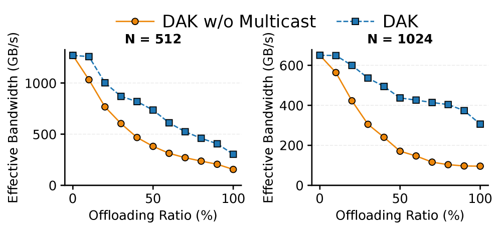<details> <summary>2604.26074v1/x21.png Details</summary>  ### Visual Description ## Line Graphs: Effective Bandwidth vs. Offloading Ratio with and without Multicast for N=512 and N=1024 ### Overview The image contains two side-by-side line graphs comparing effective bandwidth (GB/s) as a function of offloading ratio (%) for two scenarios: 1. **DAK without Multicast** (orange solid line) 2. **DAK with Multicast** (blue dashed line) Each graph corresponds to a different system size: **N = 512** (left) and **N = 1024** (right). ### Components/Axes - **X-axis**: Offloading Ratio (%) ranging from 0% to 100% (in 10% increments). - **Y-axis**: Effective Bandwidth (GB/s), scaled differently for each graph: - Left graph (N=512): 0–1200 GB/s. - Right graph (N=1024): 0–600 GB/s. - **Legends**: - Top-right of each graph. - Orange circle: "DAK w/o Multicast" - Blue dashed square: "DAK" ### Detailed Analysis #### N = 512 (Left Graph) - **DAK w/o Multicast (orange)**: - Starts at ~1200 GB/s at 0% offloading. - Decreases linearly to ~100 GB/s at 100% offloading. - Slope: ~11 GB/s per 1% offloading. - **DAK (blue dashed)**: - Starts at ~1100 GB/s at 0% offloading. - Decreases to ~300 GB/s at 100% offloading. - Slope: ~8 GB/s per 1% offloading. #### N = 1024 (Right Graph) - **DAK w/o Multicast (orange)**: - Starts at ~600 GB/s at 0% offloading. - Decreases to ~100 GB/s at 100% offloading. - Slope: ~5 GB/s per 1% offloading. - **DAK (blue dashed)**: - Starts at ~600 GB/s at 0% offloading. - Decreases to ~300 GB/s at 100% offloading. - Slope: ~3 GB/s per 1% offloading. ### Key Observations 1. **Bandwidth Degradation**: Both scenarios show a consistent decline in bandwidth as offloading increases. 2. **Multicast Benefit**: The blue dashed line (DAK with multicast) consistently outperforms the orange line (DAK without multicast) across all offloading ratios. 3. **N Dependency**: - For N=512, the bandwidth drop is steeper (11 vs. 8 GB/s per 1% offloading). - For N=1024, the drop is gentler (5 vs. 3 GB/s per 1% offloading). 4. **Convergence**: At 100% offloading, both N=512 and N=1024 systems with multicast retain ~300 GB/s, while systems without multicast drop to ~100 GB/s. ### Interpretation - **Multicast Impact**: Multicast significantly mitigates bandwidth loss during offloading, particularly at higher offloading ratios. This suggests multicast improves resource efficiency or reduces contention in distributed systems. - **Scalability**: Larger systems (N=1024) exhibit more stable bandwidth degradation, implying better scalability or optimized resource allocation at scale. - **Trade-offs**: While multicast improves performance, the absolute bandwidth for N=1024 is lower than N=512, indicating potential trade-offs between system size and raw capacity. - **Practical Implication**: Systems prioritizing offloading should leverage multicast to maintain higher effective bandwidth, especially in high-offloading scenarios. </details> Figure 13: GEMM of weights (7168,7168) and hidden states (7168, $N$ ). TMA Multicast Efficiency: Fig. 13 shows the performance benefits of TMA multicast. We measure the performance of GEMM over a $(7168,7168)$ weight matrix with a $(7168,N)$ hidden state matrix. In this setup, we scale the batch dimension $N$ (which is determined by the LLM inference batch size) from 512 to 1024. At $N=512$ , enabling TMA multicast improves performance by 1.3 $×$ compared to the non-multicast baseline. Crucially, this performance gap widens significantly to 2.5 $×$ as $N$ increases to 1024. This scaling behavior perfectly aligns with our earlier analysis (Tab. 1): as $N$ grows, independent requests to uncacheable host memory suffer from severe read amplification. By broadcasting a single fetched tile to multiple SMs on-chip, TMA multicast eliminates these redundant host-to-GPU transfers and improves performance. Kernel Alignment Efficacy: As shown in 12(b), DAK ensures that the number of assigned tiles is evenly divisible across the allocated SMs to prevent tail latencies caused by partial or unbalanced execution waves. 12(b) shows that this optimization improves throughput by up to 1.2 $×$ . ## 7 Related Work Memory Offloading for LLM Inference. Existing memory offloading systems [sheng2023flexgen, aminabadi2022deepspeed, dao2022flashattention, ren2021zero, li2025fenghuang, huang2020swapadvisor, cao2025moe] rely on a copy-based prefetching, which, as we have shown, underperforms compared to a direct-access approach. Prefetching is only advantageous if a compute-bound kernel’s bandwidth demand is lower than the interconnect capacity, leaving idle bandwidth to prestage data for subsequent memory-bound operations. However, this scenario is rare in high-throughput LLM decoding, where kernels typically saturate the interconnect or exhibit uniform compute-intensity across stages, leaving no idle bandwidth to hide later stage fetch latencies. Direct Access with Managed Memory. Previous GPU direct host access often relies on Unified Virtual Memory (UVM) [li2015evaluation, chien2019performance], which provides on-demand access via 4KB hardware page faults. However, for large-scale tensor operations, demand-paging incurs severe fault-handling latency and serialization overheads. Even on recent tightly-coupled architectures like GH200 Superchip, evaluations [schieffer2024harnessing, fusco2024understanding] show that managed memory imposes significant migration and fault-handling bottlenecks for memory-intensive workloads. DAK uses TMA to avoid paging overhead. Tensor Memory Accelerator (TMA) and Async Kernels. Libraries like CUTLASS 3 [cutlass3], ThunderKittens [spector2024thunderkittens], Mirage [cheng2025mirage], and FlashAttention-3 [shah2024flashattention] use TMA for warp-specialized pipelining. However, prior work restricts TMA to intra-GPU (HBM-to-SMEM) movement. DAK repurpose TMA for inter-tier data movement, orchestrating direct, asynchronous accesses over the host-GPU interconnect while actively mitigating remote congestion and read amplification. ## 8 Conclusion We show that direct access is better than prefetching for LLM inference offloading. We present DAK, a framework that leverages the TMA to fetch weights and KV caches directly from host memory to GPU shared memory. DAK incorporates a greedy algorithm for per-operation offloading, congestion control to prevent interconnect saturation, and TMA multicasting to eliminate read amplification. Our evaluations show that DAK strictly outperforms prefetching, achieving near-optimal system bandwidth with performance gains of up to 3 $×$ on NVLink-C2C and 1.8 $×$ on PCIe systems. ## 9 Acknowledgements This work is supported by gifts from Google, as well as resources provided by Lambda and the NAIRR Pilot. ## References ## Appendix A Formal Proof of Optimal Greedy Offload The optimization problem can be written as: $$ \displaystyle\min_\{x_{i\}} \displaystyle∑_i\frac{C_i}{EB(x_i)} \displaystyle∑_iC_ix_i=R∑_iC_i, \displaystyle 0≤ x_i≤ 1, ∀ i, \tag{1} $$ Next, we explain why the greedy algorithm proposed in § 4.2 is an optimal solution to this problem. **Theorem 1** *When $R≤\frac{∑_i∈F_memC_i· x_i^*}{∑_iC_i}$ , the optimal solution allocates all offloading budget to memory-bound operations, and how the offloading budget is distributed among memory-bound operations does not affect optimality.* * Proof* We prove this by contradiction. Suppose there exists an optimal solution in which some compute-bound operation $F_j∈F_comp$ has $x_j>0$ . Since $R≤\frac{∑_i∈F_memC_ix_i^*}{∑_iC_i}$ , there must exist at least one memory-bound operation $F_k∈F_mem$ such that $x_k<x_k^*$ ; otherwise, if every memory-bound operation had already reached its threshold, then the total offloaded size assigned to memory-bound operations alone would be at least $∑_i∈F_memC_ix_i^*$ , contradicting the above bound. Now move an infinitesimal amount of offloading budget from $F_j$ to $F_k$ , while keeping the total offloaded size unchanged. Let us use $T(x_i)=\frac{C_i}{EB(x_i)}$ to denote the latency contribution of operation $F_i$ . For the compute-bound operation $F_j$ , $T(x_i)$ is strictly non-decreasing in $x_j$ ; thus we have $T(\hat{x_j})≤ T(x_j)$ . For the memory-bound operation $T(x_i)$ is strictly decreasing when $x_i<x_i^*$ ; thus we have $T(\hat{x_k})<T(x_k)$ . Therefore, decreasing $x_j$ and increasing $x_k$ strictly decreases the objective value, contradicting the optimality of the original solution. Hence, any optimal solution satisfies the following constraint: $$ \displaystyle\begin{cases}x_i≤ x_i^*&∀ i∈F_mem\\ x_i=0&∀ i∈F_comp\end{cases} \tag{4} $$ When the constraint in 4 holds, the objective in 1 only depends on memory-bound operations. Rewriting the objective, we have $\min_\{x_{i\}}∑_i\frac{C_i(1-x_i)}{B_g}$ . Since $B_g$ is a constant, this is equivalent to minimizing $∑_iC_i(1-x_i)$ , or equivalently maximizing $∑_iC_ix_i$ . Under the global offloading constraint in 2, $∑_iC_ix_i$ is fixed. Therefore, the objective reduces to a constant, and any feasible solution satisfying the constraints is optimal. How the offloading budget is distributed among memory-bound operations does not affect optimality in this regime. ∎ **Theorem 2** *When $\frac{∑_i∈F_memC_i· x_i^*}{∑_iC_i}<R≤\frac{∑_iC_i· x_i^*}{∑_iC_i}$ , the optimal solution allocates offloading budget to all memory-bound operations so that they reach their peak effective bandwidth. It then allocates the remaining budget to compute-bound operations; the exact distribution among compute-bound operations does not affect optimality, as long as none of them is pushed beyond its compute-bound threshold.* * Proof* Since $\frac{C_i}{EB(x_i)}$ is decreasing and then increasing with $x_i$ for memory-bound operations, and strictly non-decreasing with $x_i$ for compute-bound operations. The optimal solution would assign $x_i=x_i^*$ for all memory-bound operations, minimizing their operation latency. In addition, due to the constraint on $R≤\frac{∑_iC_i· x_i^*}{∑_iC_i}$ , we can make sure no compute-bound operations go beyond their threshold. In this case, we can minimize $\frac{C_i}{EB(x_i)}$ for both memory-bound and compute-bound operations, and thus minimize the E2E latency. Thus, an optimal solution would satisfy the following constraint: $$ \displaystyle\begin{cases}x_i=x_i^*&∀ i∈F_mem\\ x_i≤ x_i^*&∀ i∈F_comp\end{cases} \tag{5} $$ Under this constraint, we can rewrite the objective 1 as $∑_i∈F_mem\frac{C_i}{B_h+B_g}+∑_i∈F_comp\frac{C_i}{B_i}$ , which is a constant. Hence, any feasible solution which satisfies Constraint 5 would be optimal. How the offloading budget is distributed among compute-bound operations does not affect optimality in this regime. ∎ **Theorem 3** *When $R>\frac{∑_iC_i· x_i^*}{∑_iC_i}$ , Any feasible solution is optimal, and how the offloading budget is distributed among all operations does not affect optimality.* * Proof* We first show show that for any optimal solution, it must satisfy $x_i≥ x_i^*,∀∈F$ . We prove this by contradiction. Suppose there exists an optimal solution $S$ in which some operation has $x_j<x_j^*$ . Due to the constraint on offloading budget $R$ , there must exist some $x_k$ with $x_k>x_k^*$ . Then consider another solution $\hat{S}$ with $\hat{x_j}=x_j^*>x_j$ . Since we increase the offloading size of operation $j$ , we can reduce the offloading size of operation $k$ while satisfying the overall offloading budget constraint for $\hat{S}$ . Thus, we have $\hat{x_k}<x_k$ . Note that the effective bandwidth $EB(x_i)$ is non-decreasing with $x_i≤ x_i^*$ and strictly decreasing with $x_i>x_i^*$ . Thus, the latency of operation $j$ in solution $\hat{S}$ would be no greater than its latency in solution $S$ , and the latency of operation $k$ in solution $\hat{S}$ would be smaller than its latency in solution $S$ , contradicting the assumption that $S$ is optimal. Thus, we can rewrite the objective 1 as $∑_i∈F_mem\frac{C_i}{B_h}· x_i+∑_i∈F_comp\frac{C_i}{B_i}· x_i=∑_i∈F_mem{C_i}· x_i+∑_i∈F_compC_i· x_i=∑_i∈FC_i· x_i$ , which is a constant, i.e., the total offloading budget (due to constraint 2). Putting everything together, our offloading algorithm satisfies constraint 4 in Phase 1 and constraint 5 in Phase 2 respectively, making it optimal. In Phase 3, any feasible allocation is optimal. Therefore, the proposed offloading algorithm is optimal. 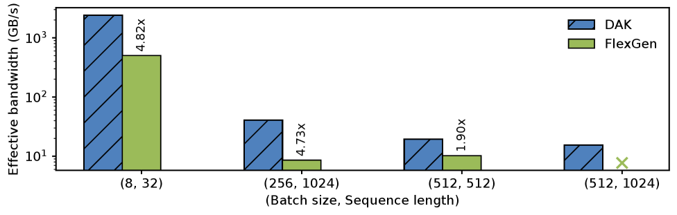∎ <details> <summary>2604.26074v1/x22.png Details</summary>  ### Visual Description ## Bar Chart: Effective Bandwidth Comparison Between DAK and FlexGen ### Overview The chart compares the effective bandwidth (in GB/s) of two methods, DAK and FlexGen, across four configurations of batch size and sequence length. The y-axis uses a logarithmic scale (10^1 to 10^3), and the x-axis categorizes configurations as (Batch size, Sequence length). Each configuration has two bars: DAK (blue with diagonal stripes) and FlexGen (green). A legend in the top-right corner identifies the methods. ### Components/Axes - **Y-axis**: "Effective bandwidth (GB/s)" with logarithmic scale (10^1 to 10^3). - **X-axis**: Four configurations: 1. (8, 32) 2. (256, 1024) 3. (512, 512) 4. (512, 1024) - **Legend**: Top-right corner, labels: - Blue (diagonal stripes): DAK - Green: FlexGen ### Detailed Analysis 1. **(8, 32)**: - DAK: ~1000 GB/s (bar height near 10^3). - FlexGen: ~500 GB/s (bar height between 10^2 and 10^3). - Multipliers: DAK = 4.82x, FlexGen = 4.73x. 2. **(256, 1024)**: - DAK: ~50 GB/s (bar height near 10^1.7). - FlexGen: ~10 GB/s (bar height near 10^1). - Multipliers: DAK = 4.73x, FlexGen = 1.90x. 3. **(512, 512)**: - DAK: ~20 GB/s (bar height near 10^1.3). - FlexGen: ~10 GB/s (bar height near 10^1). - Multipliers: DAK = 1.90x, FlexGen = 1.90x. 4. **(512, 1024)**: - DAK: ~10 GB/s (bar height near 10^1). - FlexGen: No data (marked with "X"). - Multipliers: DAK = 1.90x, FlexGen = N/A. ### Key Observations - **DAK consistently outperforms FlexGen** in all configurations where data is available. - **Effective bandwidth decreases** as batch size and sequence length increase for both methods. - **Multipliers** (likely indicating performance gains relative to a baseline) decrease with larger configurations, suggesting diminishing returns. - **FlexGen lacks data** for the (512, 1024) configuration, marked with an "X". ### Interpretation The data suggests that **DAK is more efficient** than FlexGen across tested configurations, with the largest performance gap in smaller setups (e.g., 4.82x multiplier in (8,32)). As configurations scale, both methods experience reduced bandwidth, but DAK maintains a higher relative performance. The absence of FlexGen data in the largest configuration (512,1024) may indicate technical limitations or instability under those parameters. The logarithmic y-axis emphasizes the exponential drop in bandwidth with increased computational demands. </details> | 8 256 512 | 32 1024 512 | 13.3 GB 13.3 GB 13.3 GB | 0.27 GB 141.73 GB 146.03 GB | 0% 37% 39% | | --- | --- | --- | --- | --- | | 512 | 1024 | 13.3 GB | 283.47 GB | 67% | Figure 14: Figure shows the performance for GH200 under different configurations. The table shows the memory footprint for different configurations and the corresponding global memory offload ratio. ## Appendix B Additional Results Fig. 14 shows the OPT 6.7B’s performance for GH200 under different configurations. We vary the batch size and prompt length for OPT-6.7B. Large batch sizes and extended prompt lengths increase the total memory footprint well beyond the available GPU HBM, which dynamically dictates the required global offload ratio. DAK achieves 1.9x to 4x performance improvement compared to FlexGen.