# Beyond the Baseband: Adaptive Multi-Band Encoding for Full-Spectrum Bioacoustics Classification
**Authors**: Eklavya Sarkar, Marius Miron, David Robinson, Gagan Narula, Milad Alizadeh, Ellen Gilsenan-McMahon, Felix Effenberger, Emmanuel Chemla, Olivier Pietquin, Matthieu Geist
## Abstract
Animals hear and vocalize across frequency ranges that differ substantially from humans, often extending into the ultrasonic domain. Yet most computational bioacoustics systems rely on audio models pre-trained at 16 kHz, restricting their usable bandwidth to the 0-8 kHz baseband and discarding higher-frequency information present in many bioacoustic recordings. We investigate a multi-band encoding framework that decomposes the full spectrum of animal calls into band features and fuses them into a unified representation. Similarity analyses on models show that certain encoders produce decorrelated band embeddings that improve class separation after fusion. Classification experiments on three bioacoustic datasets using eight pre-trained models and five fusion strategies show that fused representations consistently outperform the baseband and time-expansion baselines on two datasets, showing the potential of multi-band methods for full-spectrum encoding of animal calls.
footnotetext: Corresponding author: eklavya@earthspecies.org
## 1 Introduction
Bioacoustics, the study of animal sounds, has emerged as a prominent domain within machine learning, as a means to study the origins and evolution of language and vocal learning [hurford2012language, fitch2018biology], and deepen our understanding of communication in the natural world. Computational bioacoustics aims to ‘decode’ animal vocalizations to gain insights into their communication by deriving information from their calls [bioacoustics_roadmap]. In recent years, neural representations learnt on human speech have shown remarkable transferability to the domain of bioacoustics for decoding non-human vocal communication [Sarkar_Thesis_2025, cauzinille25_phd, miron2026what]. Indeed, modern state-of-the-art foundation models pre-trained on human speech and/or general audio have achieved strong performance benchmark across a range of species for tasks such as call detection [BEANS, aves, semenzin2025dolphvec], call-type classification [kloots24_vihar, shi24_vihar, mahoud24_vihar, abzaliev24, Sarkar_ICASSP_2025], or caller identification [sarkar23_interspeech, cauzinille24_interspeech, Knight2024], thus providing a reliable framework for bioacoustics tasks, and significantly advancing the field.
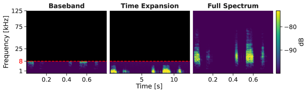
However, a critical limitation in leveraging these models is that they are typically pre-trained at a 16 kHz sampling rate (SR), corresponding to the human audible range, and resample any input to the constrained 0–8 kHz baseband, including bioacoustic recordings. As depicted in Figure 1, this bandwidth (BW) is highly insufficient to cover the higher frequency content contained in the full-spectrum of many animals and their vocalizations, which extend well beyond this threshold, and results in a significant loss of useful information. For example, bat echolocation calls can reach up to 200 kHz [bats_altringham], insect signals to 100 kHz [drosopoulos2005insect], and marine mammal calls to 150 kHz [berta2005marine]. However, training entire foundation models at higher SRs is very computationally expensive, and only a few such models exist, such as BirdNET [kahl2021birdnet] and Perch [Ghani2023, perch2], pre-trained at 48 and 32 kHz, respectively, on bioacoustics. Thus, the fixed pre-training bandwidth of existing audio models is a major limitation in all current computational bioacoustics works.
A common signal-processing approach to address this problem is time-expansion, i.e. slowing down the audio recordings by a fixed factor to shift the high-frequency components down to the baseband of the pre-trained model [preatoni2005identifying, kershenbaum2025automatic, bats2000], and using the resulting signal as input. However, this approach considerably reduces the spectral resolution and proportionally stretches the recording, as illustrated in Figure 1 (middle), thus increasing the model’s computational cost of processing the signal.
<details>
<summary>2604.27936v1/x1.png Details</summary>
### Visual Description
## Spectrogram Analysis: Signal Processing Stages
### Overview
The image presents three sequential stages of signal processing visualization: Baseband, Time Expansion, and Full Spectrum. Each plot uses a spectrogram-like representation with frequency (kHz) on the y-axis and time (s) on the x-axis. Color intensity corresponds to signal strength (dB), with a colorbar indicating values from -90 dB (dark purple) to -80 dB (bright yellow).
### Components/Axes
1. **Baseband Plot**
- **Y-axis**: Frequency [kHz] (1–125 kHz)
- **X-axis**: Time [s] (0.2–0.6 s)
- **Key Feature**: Red dashed line at 8 kHz
- **Color Scale**: Minimal activity (purple/blue) below 8 kHz
2. **Time Expansion Plot**
- **Y-axis**: Frequency [kHz] (1–125 kHz)
- **X-axis**: Time [s] (0–10 s)
- **Key Feature**: Red dashed line at 8 kHz
- **Color Scale**: Increased activity (yellow/green) near 8 kHz
3. **Full Spectrum Plot**
- **Y-axis**: Frequency [kHz] (1–125 kHz)
- **X-axis**: Time [s] (0.2–0.6 s)
- **Color Scale**: Detailed peaks (yellow/green) across 8–125 kHz
- **Legend**: Right-aligned colorbar labeled "dB" (-90 to -80 dB)
### Detailed Analysis
- **Baseband**: Dominated by black (no signal) except for faint purple/blue streaks below 8 kHz. The red dashed line at 8 kHz acts as a reference threshold.
- **Time Expansion**: Expanded time axis reveals intermittent yellow/green pulses near 8 kHz, suggesting transient events or harmonics.
- **Full Spectrum**: Highest detail with vertical yellow/green peaks clustered around 8 kHz and higher frequencies (up to ~125 kHz). Peaks show dB values approaching -80 dB.
### Key Observations
1. **Threshold Significance**: The 8 kHz red line likely represents a critical frequency cutoff or modulation boundary.
2. **Temporal Evolution**: Time Expansion reveals hidden spectral content absent in Baseband, indicating time-domain processing (e.g., modulation/demodulation).
3. **Spectral Detail**: Full Spectrum shows sharp, narrowband peaks (e.g., ~8 kHz, ~20 kHz, ~50 kHz) with dB values up to -80 dB, suggesting structured modulation (e.g., OFDM, FSK).
### Interpretation
The progression from Baseband to Full Spectrum demonstrates:
- **Baseband Limitation**: Original signal is band-limited below 8 kHz, with weak sub-harmonic content.
- **Time Expansion Role**: Temporal stretching uncovers higher-frequency components, possibly through nonlinear processing or sampling rate conversion.
- **Full Spectrum Insight**: Reveals intentional modulation schemes with distinct carrier frequencies and sidebands. The 8 kHz peak may represent a fundamental tone, while higher peaks (20–50 kHz) suggest harmonics or subcarriers.
Notably, the absence of activity above 125 kHz in all plots implies an anti-aliasing filter or sampling rate constraint. The consistent 8 kHz reference across plots suggests it is a design parameter (e.g., sampling frequency divided by 16 for a 128 kHz sample rate).
</details>
Figure 1: Spectrograms of an ultrasonic bat vocalization.
Inspired by classical sub-band processing approaches in automatic speech recognition (ASR), where the signal is decomposed into frequency bands that are processed independently before combining their evidence to improve robustness [bourlard1996mew, bourlard1996multi, tibrewala1997multi, hermansky1998traps], we investigate an adaptive multi-band (MB) encoding strategy for bioacoustics. Unlike in ASR, where such methods operated on sub-bands within the 0–8 kHz baseband, we instead decompose the full spectrum of animal vocalizations into multiple basebands, compatible with modern pre-trained audio models, and explore combining them into a unified representation through various fusion strategies. Based on this proposed approach, this paper investigates the following two central questions:
1. Can MB representations effectively exploit the unused high-frequency information in bioacoustic calls, and improve over the conventional baseband and time-expansion approaches?
1. How does this approach compare to simply using the baseband of a model trained at a higher SR, such as BirdNET, at 48 kHz? Moreover, when applied to such a model, does it yield additional gains over its application to standard 16 kHz models?
To answer these questions, we conduct a systematic evaluation across multiple bioacoustics datasets and pre-trained audio models. It is to be noted that we do not provide a foundation model pre-trained for higher SRs in this paper, but instead propose an approach that can work with any existing model. To provide practical use to the bioacoustics community, we also release the framework as an open-source toolkit. Source code: https://github.com/earthspecies/multiband-audio.
The rest of this paper is organized as follows. Section 2 details the MB encoding approach, and section 3 gives our experimental setup. Section 4 – 5 respectively present a representation and classification analysis. Section 6 concludes the paper.
## 2 Adaptive Multi-Band Encoding
<details>
<summary>2604.27936v1/x2.png Details</summary>
### Visual Description
## Flowchart: Signal Processing and Machine Learning Pipeline
### Overview
The diagram illustrates a two-stage pipeline for processing raw vocalizations into model outputs. The top section shows signal preprocessing steps, while the bottom section depicts a machine learning model architecture. The flow progresses from left to right, with preprocessing feeding into the model's feature extraction and fusion stages.
### Components/Axes
**Top Section (Preprocessing):**
- **Input:** Raw vocalization `s` (black squiggly line)
- **Processing Steps (orange boxes):**
1. Band-pass filter
2. Heterodyne
3. Low-pass filter
4. Resample
- **Output:** `B` baseband waveforms (black squiggly lines with arrow)
**Bottom Section (Model Pipeline):**
- **Input:** Results `ŷ` (gray box)
- **Components:**
1. Classifier (blue box)
2. Linear layer (pink rectangle)
3. Representation `x` (black arrow)
4. Fusion (teal box)
- Sub-components:
- Mean-pooling (light blue rectangle)
- Functionals `f` (orange rectangle)
5. Model `F` (pink circle)
- **Output:** Final model output (black arrow from `F`)
**Legend/Color Coding:**
- Orange: Preprocessing filters
- Blue: Classifier
- Pink: Linear layer/model
- Teal: Fusion
- Light blue/orange: Fusion sub-components
### Detailed Analysis
**Preprocessing Flow:**
1. Raw vocalization passes through sequential filters (band-pass → heterodyne → low-pass) before resampling
2. Output is baseband waveforms `B` with multiple frequency components (three waveform examples shown)
**Model Pipeline:**
1. Classifier processes results `ŷ` through a linear layer
2. Output representation `x` feeds into fusion module
3. Fusion combines mean-pooling features with learned functionals `f`
4. Final model `F` synthesizes fused features for final output
### Key Observations
1. **Signal Conditioning:** Preprocessing focuses on frequency domain manipulation (filtering, resampling)
2. **Feature Hierarchy:** Model pipeline progresses from raw results → linear features → fused representations
3. **Modular Design:** Fusion module explicitly separates mean-pooling from learned functionals
4. **Color Consistency:** Orange dominates preprocessing, while model components use cooler tones (blue/pink/teal)
### Interpretation
This architecture suggests a hybrid approach combining traditional signal processing with modern machine learning:
- **Preprocessing Stage:** Prepares raw audio for feature extraction through analog-style filtering techniques
- **Model Stage:** Employs a classifier with linear features, then enhances through fusion of handcrafted (mean-pooling) and learned (functionals) features
- **Model F:** Likely represents a non-linear decision boundary or generative model operating on fused features
The separation of mean-pooling (static feature) and functionals (learned features) in the fusion module implies an attention mechanism or feature weighting system. The use of baseband waveforms as input to the classifier suggests frequency-domain feature extraction precedes temporal processing in the model.
</details>
Figure 2: Complete pipeline of the heterodyning-based multi-band encoding.
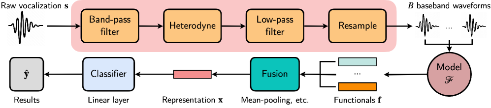
This section details the heterodyning-based multi-band processing approach, illustrated in Figure 2. It consists of three main stages: (i) spectral band decomposition and baseband mapping, (ii) per-band representation extraction using a frozen pre-trained encoder, and (iii) fusion of the resulting band-level representations into a unified embedding for downstream classification.
Given a raw audio recording $s$ sampled at its native rate $f_s$ , a pre-trained model operating at $f_m$ can only access frequencies up to its Nyquist $f_m/2$ . To leverage the higher spectral information $s$ , we split its full spectrum into $B=\lceil f_s/f_m\rceil$ non-overlapping bands of width $f_m/2$ . The first band ( $0$ – $f_m/2$ Hz) corresponds to the standard baseband, and is not further processed. For each subsequent band $b$ , we first extract the corresponding spectral slice by applying a band-pass filter to the raw signal $s$ , yielding $s_b$ centered at frequency $f_b$ . We then heterodyne it down to the baseband by multiplying it by a cosine at the band’s center frequency $f_b$ , followed by low-pass filtering $H_LP$ . The resulting baseband signal $\bar{s}_b$ is given by:
$$
\bar{s}_b=H_LP\bigl[s_b·\cos(2π f_bt)\bigr]
$$
Applying this to each band produces $B$ baseband waveforms $\bar{S}=\{\bar{s}_1,…,\bar{s}_B\}$ , each representing a distinct portion of the original spectrum. We resample them to $f_m$ , matching the SR expected by the pre-trained model, and then pass them individually through the frozen encoder $F$ , yielding $B$ variable-length multi-dimensional embeddings. These are then transformed into $B$ fixed-length vocalization-level functionals $f_b∈ℝ^D$ by computing the first-order statistics across the temporal axis, where $D$ denotes the embedding dimension of the model. Finally, a learned fusion module combines these functionals into a final representation $x∈ℝ^D$ , on which a linear classifier is trained for the downstream task. In this paper, we investigate five distinct fusion strategies, detailed below:
- Mean-Pool (MP): $f$ are averaged element-wise across the band dimension, assigning equal weight coefficients to all frequency bands. No new learnable parameters are introduced.
- Gated-Pool (GP): A linear projection maps each $f_b$ to a scalar score, which is normalized via softmax to produce band-level weights coefficients $w_b$ . The fused representation is the weighted sum of the band functionals $x=∑_bw_bf_b$ , allowing the model to learn which frequency bands are most informative.
- Mixture-of-Experts (MoE): Each $f_b$ is passed through an independent linear classifier head to obtain band-level logits $z_b$ . A separate 2-layer MLP computes band-level weights coefficients from $f_b$ . The final prediction is the weighted sum of band logits $\hat{y}=∑_bw_bz_b$ . Unlike GP, which fuses $f$ before classification, MoE classifies them first and fuses the resulting logits.
- Hybrid (HYB): Similar to GP, but the gating network additionally incorporates handcrafted features, namely spectral entropy and flux, alongside each $f_b$ to compute band weight coefficients. The concatenated representation is input to a 3-layer MLP, enabling the gating decision to leverage both the learned functionals and acoustic properties of each band.
- Self-Attention (SA): $f$ are treated as a sequence of tokens, with a learnable [CLS] token and positional embeddings. A single-layer transformer encoder processes the sequence, contextualizing each band’s representation with all other bands through a multi-head attention mechanism. The [CLS] output serves as the fused representation $x$ .
## 3 Experimental Setup
### 3.1 Datasets, Tasks, and Protocols
We investigate our method on three distinct bioacoustic datasets (DS) in the BEANS [BEANS] benchmark, summarized in Table 1.
Table 1: SR is given in kHz. $S$ is the # of samples, $L$ length [mins.], $n_c$ # of classes, $μ$ median length [s], $σ$ std, and $B$ the number of 8 kHz bands.
| Dogs CBI Bats | $44.1$ $44.1$ $250$ | $688$ $21$ K $10$ K | $126$ $3351$ $313$ | $10$ $264$ $10$ | $8.05$ $10.00$ $1.45$ | $16.01$ $1.70$ $1.08$ | 3 3 16 |
| --- | --- | --- | --- | --- | --- | --- | --- |
The downstream tasks consist of caller identity classification for Dogs and Bats, and species classification for Cornell Birdcall Identification (CBI). We follow the protocols defined in BEANS to split the datasets into Train, Val, and Test sets.
### 3.2 Models, Feature Representations, and Baselines
For our work, we consider different families of pre-trained (PT 0) models to obtain distinct features $F$ . They are post-trained (PT 1) on various dataset permutations, given in Table 2.
Table 2: # Parameters $P$ [M] and feature dimension $D$ of models. IN represents ImageNet, AS AudioSet, XC Xeno-Canto.
| EffNet-Bio | SL | IN | SL | Bio | 5 | 1280 |
| --- | --- | --- | --- | --- | --- | --- |
| EffNet-AS | SL | IN | SL | AS | 5 | 1280 |
| EffNet-All | SL | IN | SL | All | 5 | 1280 |
| BEATs-Bio | SSL | AS | SL | Bio | 91 | 768 |
| BEATs-All | SSL | AS | SL | All | 91 | 768 |
| BEATs-NLM | SSL | AS | ALM | Misc | 91 | 768 |
| EATs-All | SSL | AS | SL | Bio | 90 | 768 |
| EATs-Bio | SSL | AS | SL | Bio | 90 | 768 |
| BirdNET | SL | XC | – | – | 14 | 1024 |
SL pre-trained on ImageNet: We select EfficientNet for its moderate size and strong performance on BEANS [miron2026what]. It is a 16 kHz CNN model pre-trained on ImageNet. We evaluate three variants https://github.com/earthspecies/avex. post-trained on bioacoustics data (Bio), AudioSet (AS), or both (All) [miron2026what] to assess the impact of the post-training domain for leveraging higher-frequency content. We also include BirdNET, a 48 kHz model based on the same architecture and post-trained primarily on Xeno-Canto (XC), to directly compare performance across BWs and test if our multi-band approach generalizes to models with higher native SRs.
SSL pre-trained on speech and general audio: BEATs is a larger model composed of a CNN module operating on mel-spectrogram input patches, followed by 12 transformer layers. We pick two variants post-trained on Bio and All, and Nature-LM audio’s BEATS encoder, extracted from an audio-language model (ALM) trained on bioacoustic audio and text pairs [naturelm].
SSL pre-trained on human speech, general audio, and bioacoustics: EATs is a SSL pre-trained with teacher distillation and masked spectrogram reconstruction tasks on Bio, AS, and All sets. We select the variants post-trained on Bio and All.
For all the models, we extract the final encoder layer. We compare our multi-band approach with the following baselines.
- Baseband (BB): we simply resample $s$ to the given model’s baseband, and lose any spectral content above this threshold.
- Time-Expansion (TE): we slow down $s$ to shift and compress all the spectral information down to the model’s baseband.
## 4 Representation Analysis
This section presents similarity analysis of the extracted features $x$ . For these studies we only work with the Train set.
### 4.1 Band Discrimination
<details>
<summary>2604.27936v1/x3.png Details</summary>
### Visual Description
## Heatmap: Cosine Similarity Across Frequency Bands and Models
### Overview
The image is a heatmap visualizing cosine similarity values between different audio processing models (EffNet, BEATs, EAT) and frequency bands (0-8 kHz to 120-125 kHz). The color scale ranges from red (low similarity, ~0.0) to green (high similarity, ~1.0). A "TE" row at the bottom contains negative values, suggesting a distinct metric or anomaly.
### Components/Axes
- **X-axis (Models/Datasets)**:
EffNet All, EffNet Bio, EffNet AS, BEATs All, BEATs Bio, BEATs NLM, EAT All, EAT Bio.
- **Y-axis (Frequency Bands)**:
0-8 kHz, 8-16 kHz, 16-24 kHz, 24-32 kHz, 32-40 kHz, 40-48 kHz, 48-56 kHz, 56-64 kHz, 64-72 kHz, 72-80 kHz, 80-88 kHz, 88-96 kHz, 96-104 kHz, 104-112 kHz, 112-120 kHz, 120-125 kHz, TE.
- **Legend**:
Color gradient from red (0.0) to green (1.0), labeled "Cosine Sim."
### Detailed Analysis
- **Frequency Bands**:
- **0-8 kHz**: All values are 1.00 (green), indicating perfect similarity within this band.
- **8-16 kHz**: Values range from 0.39 (EffNet Bio) to 0.92 (EAT All).
- **16-24 kHz**: Values range from 0.48 (EffNet Bio) to 0.93 (EAT All).
- **24-32 kHz**: Values range from 0.43 (EffNet Bio) to 0.91 (EAT All).
- **32-40 kHz**: Values range from 0.39 (EffNet Bio) to 0.90 (EAT All).
- **40-48 kHz**: Values range from 0.35 (EffNet Bio) to 0.89 (EAT All).
- **48-56 kHz**: Values range from 0.32 (EffNet Bio) to 0.88 (EAT All).
- **56-64 kHz**: Values range from 0.29 (EffNet Bio) to 0.87 (EAT All).
- **64-72 kHz**: Values range from 0.25 (EffNet Bio) to 0.85 (EAT All).
- **72-80 kHz**: Values range from 0.22 (EffNet Bio) to 0.84 (EAT All).
- **80-88 kHz**: Values range from 0.16 (EffNet Bio) to 0.82 (EAT All).
- **88-96 kHz**: Values range from 0.15 (EffNet Bio) to 0.81 (EAT All).
- **96-104 kHz**: Values range from 0.13 (EffNet Bio) to 0.80 (EAT All).
- **104-112 kHz**: Values range from 0.10 (EffNet Bio) to 0.79 (EAT All).
- **112-120 kHz**: Values range from 0.06 (EffNet Bio) to 0.79 (EAT All).
- **120-125 kHz**: Values range from 0.13 (EffNet Bio) to 0.81 (EAT All).
- **TE**: Contains negative values (-0.03 to -0.04), suggesting a distinct metric or error.
- **Models/Datasets**:
- **EffNet All**: Consistently high similarity (1.00) in 0-8 kHz, decreasing to 0.19 in 120-125 kHz.
- **EffNet Bio**: Lower similarity across all bands (e.g., 0.39 in 8-16 kHz, 0.06 in 112-120 kHz).
- **EffNet AS**: Moderate similarity (e.g., 0.67 in 8-16 kHz, 0.67 in 120-125 kHz).
- **BEATs All**: High similarity (e.g., 0.52 in 8-16 kHz, 0.46 in 120-125 kHz).
- **BEATs Bio**: Lower similarity (e.g., 0.16 in 80-88 kHz, 0.47 in 120-125 kHz).
- **BEATs NLM**: Moderate similarity (e.g., 0.60 in 8-16 kHz, 0.59 in 120-125 kHz).
- **EAT All**: Highest similarity in most bands (e.g., 0.92 in 8-16 kHz, 0.81 in 120-125 kHz).
- **EAT Bio**: Moderate similarity (e.g., 0.57 in 8-16 kHz, 0.50 in 120-125 kHz).
### Key Observations
1. **Frequency Band Trends**:
- Similarity decreases with increasing frequency bands for most models.
- **EAT All** maintains the highest similarity across all bands, while **EffNet Bio** shows the lowest.
- The **TE** row contains negative values, which deviate from the rest of the data.
2. **Model Performance**:
- **EAT All** and **EffNet All** exhibit the highest similarity in lower frequency bands (0-8 kHz).
- **BEATs NLM** and **EffNet AS** show moderate similarity, particularly in mid-to-high frequency bands.
- **EffNet Bio** and **BEATs Bio** consistently underperform compared to their "All" counterparts.
3. **Anomalies**:
- The **TE** row’s negative values (-0.03 to -0.04) are outliers, possibly indicating a different calculation or error.
### Interpretation
The heatmap demonstrates that **EAT All** and **EffNet All** models achieve the highest cosine similarity, particularly in lower frequency bands (0-8 kHz), where values reach 1.00. As frequency increases, similarity generally declines, with **EffNet Bio** and **BEATs Bio** showing the weakest performance. The **TE** row’s negative values suggest a potential anomaly or a distinct metric not aligned with the rest of the data. This could imply that the "TE" category measures a different aspect of similarity or contains errors. The consistent decline in similarity with higher frequency bands highlights the challenges of audio processing in higher frequency ranges across all models.
</details>
Figure 3: Mean cosine similarity between baseband and other band’s embeddings for Bats. Higher (greener) values indicate closer representational similarity with the baseband.
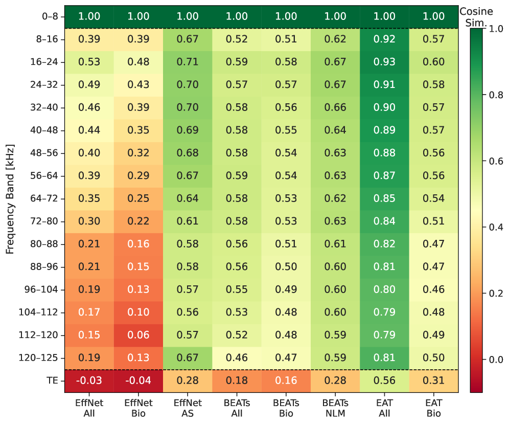
We first explore how the extracted features vary across frequency bands, given that none of the models were exposed to high-frequency content during PT 0 or PT 1. To that end, Figure 3 shows the mean cosine similarity between the baseband (0–8 kHz) and the embeddings extracted from all the other frequency bands, post-heterodyning, for the Bats dataset. For EffNet-All and Bio, we can notably observe that the similarity decreases progressively with higher frequency bands, indicating that they produce representations increasingly decorrelated from the baseband, which could benefit the fusion methods by adding complementary information. In contrast, EAT-All maintains consistently high similarity across the frequency spectrum, implying that features from different bands are encoded very similarly to the baseband. The remaining models also only show moderate similarity with the baseband, with some variation across bands. TE yields near-zero or negative scores, showing that compressing the entire 125 kHz spectrum into the 8 kHz baseband via a 15.6x time-expansion produces fundamentally different representations. Dogs and CBI features yield similar overall patterns, suggesting similar behavior for band similarity.
### 4.2 Class Separation
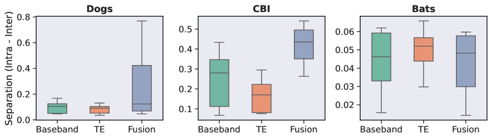
We also investigate the class discrimination of the extracted representations. To this end, we compute the pairwise mean intra and inter-class cosine similarities, and measure their separation as the difference between the two. In an ideal scenario, intra-class similarity is high and inter-class similarity is low, yielding a high class separation value. Figure 4 visualizes the resulting class-separation scores for each approach, aggregated across all models. The fusion distributions are taken from all strategies.
<details>
<summary>2604.27936v1/x4.png Details</summary>
### Visual Description
## Box Plot: Separation Metrics by Method and Category
### Overview
The image presents three box plots comparing separation metrics (Intra - Inter) across three categories: Dogs, CBI, and Bats. Each category is analyzed using three methods: Baseband, TE, and Fusion. The plots visualize median values, interquartile ranges, and outliers for each combination.
### Components/Axes
- **X-axis**: Methods (Baseband, TE, Fusion)
- **Y-axis**: Separation (Intra - Inter) values, scaled differently per category:
- Dogs: 0.0–0.8
- CBI: 0.0–0.5
- Bats: 0.0–0.06
- **Legend**:
- Green = Baseband
- Orange = TE
- Blue = Fusion
### Detailed Analysis
#### Dogs
- **Baseband (Green)**: Median ≈ 0.1, range 0.05–0.15
- **TE (Orange)**: Median ≈ 0.05, range 0.02–0.1
- **Fusion (Blue)**: Median ≈ 0.4, range 0.3–0.7
#### CBI
- **Baseband (Green)**: Median ≈ 0.3, range 0.1–0.4
- **TE (Orange)**: Median ≈ 0.2, range 0.15–0.3
- **Fusion (Blue)**: Median ≈ 0.45, range 0.35–0.5
#### Bats
- **Baseband (Green)**: Median ≈ 0.04, range 0.02–0.06
- **TE (Orange)**: Median ≈ 0.05, range 0.03–0.06
- **Fusion (Blue)**: Median ≈ 0.045, range 0.03–0.06
### Key Observations
1. **Dogs**: Fusion achieves the highest separation (median 0.4), significantly outperforming Baseband and TE.
2. **CBI**: Fusion also leads (median 0.45), with Baseband and TE showing moderate separation.
3. **Bats**: All methods yield nearly identical separation (medians 0.04–0.05), with minimal variation.
4. **Outliers**: No explicit outliers marked, but Fusion in Dogs has a notably wide range (0.3–0.7).
### Interpretation
- **Method Effectiveness**: Fusion consistently improves separation in Dogs and CBI, suggesting it captures critical inter/intra-group distinctions better than Baseband or TE.
- **Category-Specific Performance**: Bats show negligible separation across methods, implying inherent similarity in intra/inter-group metrics for this category.
- **Uncertainty**: Approximate values (e.g., medians) are inferred from box plot positions; exact numerical data is not provided.
- **Design Insight**: The use of distinct colors (green, orange, blue) aligns with the legend, ensuring clarity in method differentiation.
This analysis highlights Fusion as a robust method for enhancing separation in Dogs and CBI, while Bats exhibit uniform performance across all methods.
</details>
Figure 4: Class separation per method. Higher values indicates more discriminative embeddings.
For Dogs, fusion shows high variance across models. The median separation is comparable to BB and TE, but some models achieve substantially higher scores, indicating that fusion can yield more discriminative representations for certain models. For CBI, fusion shows a clear improvement over both methods. Finally, for Bats, all methods show comparable separation, with TE achieving a marginally higher median. As shown in Figure 3, most models encode higher frequency bands similarly to the baseband, meaning fusion combines largely redundant representations. In contrast, TE produces near-orthogonal features that yield slightly better class separation.
## 5 Classification Results
This section analyzes the downstream classification performance of the extracted features, using a linear head trained for 20 epochs. We evaluate the performance with accuracy on Test.
<details>
<summary>2604.27936v1/x5.png Details</summary>
### Visual Description
## Bar Chart: Performance Comparison Across Models and Frequency Bands
### Overview
The image presents a comparative bar chart analyzing performance metrics across three frequency bands (Dogs at 44 kHz, CBI at 44 kHz, and Bats at 250 kHz) for various audio processing models. Two data series are compared: "TE" (green bars) and "Best Fusion" (yellow bars), with numerical values indicating performance differences from a baseline.
### Components/Axes
- **X-Axis**: Model categories:
- EffNet All
- EffNet Bio
- EffNet AS
- BEATs All
- BEATs Bio
- BEATs NLM
- EAT All
- EAT Bio
- BirdNET
- **Y-Axes**:
- **Dogs (44 kHz)**: Range -10 to +10 (44 kHz)
- **CBI (44 kHz)**: Range -30 to +10 (44 kHz)
- **Bats (250 kHz)**: Range 0 to +15 (250 kHz)
- **Legend**:
- Green = TE
- Yellow = Best Fusion
- **Positioning**: Legend located in the bottom-right corner. Bars are clustered by model category across the three y-axes.
### Detailed Analysis
#### Dogs (44 kHz)
- **EffNet All**: TE = -5.8, Best Fusion = +3.6
- **EffNet Bio**: TE = +0.0, Best Fusion = +2.9
- **EffNet AS**: TE = +7.9, Best Fusion = +5.8
- **BEATs All**: TE = +0.7, Best Fusion = +2.2
- **BEATs Bio**: TE = -5.0, Best Fusion = +0.0
- **BEATs NLM**: TE = -0.7, Best Fusion = +0.0
- **EAT All**: TE = -8.6, Best Fusion = +0.7
- **EAT Bio**: TE = -3.6, Best Fusion = +2.9
- **BirdNET**: TE = 0.0, Best Fusion = N/A
#### CBI (44 kHz)
- **EffNet All**: TE = -17.7, Best Fusion = +1.0
- **EffNet Bio**: TE = -15.6, Best Fusion = +0.8
- **EffNet AS**: TE = +4.0, Best Fusion = +7.7
- **BEATs All**: TE = -16.4, Best Fusion = +0.6
- **BEATs Bio**: TE = -14.3, Best Fusion = +0.3
- **BEATs NLM**: TE = -11.7, Best Fusion = +7.1
- **EAT All**: TE = -26.4, Best Fusion = +1.7
- **EAT Bio**: TE = -25.3, Best Fusion = +0.5
- **BirdNET**: TE = 0.0, Best Fusion = N/A
#### Bats (250 kHz)
- **EffNet All**: TE = +9.4, Best Fusion = +8.3
- **EffNet Bio**: TE = +10.2, Best Fusion = +7.2
- **EffNet AS**: TE = +14.9, Best Fusion = +9.5
- **BEATs All**: TE = +8.6, Best Fusion = +3.5
- **BEATs Bio**: TE = +9.0, Best Fusion = +3.9
- **BEATs NLM**: TE = +8.6, Best Fusion = +2.5
- **EAT All**: TE = +9.8, Best Fusion = +2.0
- **EAT Bio**: TE = +7.9, Best Fusion = +4.7
- **BirdNET**: TE = +3.8, Best Fusion = +1.4
### Key Observations
1. **Best Fusion Outperforms TE**: In all categories except BirdNET (no Best Fusion data), yellow bars (Best Fusion) show higher values than green bars (TE).
2. **CBI Band Extremes**:
- Most negative TE values occur in EAT All (-26.4) and EAT Bio (-25.3).
- Best Fusion shows minimal improvement in CBI (max +7.7 in EffNet AS).
3. **Bats Band Dominance**:
- EffNet AS achieves the highest TE value (+14.9) and Best Fusion (+9.5).
- BirdNET underperforms compared to other models in this band.
4. **Mixed Performance in Dogs**:
- EffNet AS shows strong TE performance (+7.9), but Best Fusion lags (+5.8).
- EAT All has the worst TE performance (-8.6) but slight Best Fusion improvement (+0.7).
### Interpretation
The data suggests that **Best Fusion** consistently improves performance across models and frequency bands compared to TE, with the most significant gains observed in the **Bats (250 kHz)** band. However, **CBI (44 kHz)** reveals critical weaknesses in TE performance, particularly for EAT models, where Best Fusion only partially mitigates losses. The **EffNet AS** model emerges as the strongest performer in Bats, while **EAT All** exhibits the most severe TE underperformance in CBI. BirdNET's absence in the Best Fusion comparison for CBI and Dogs raises questions about its applicability or data availability. The stark contrast between TE and Best Fusion in CBI highlights potential architectural or fusion strategy advantages in the latter approach.
</details>
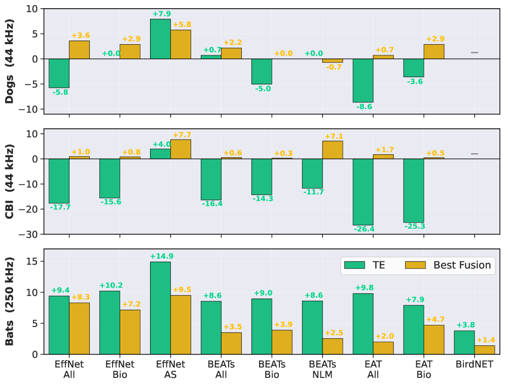
Figure 5: Test classification accuracy gain over baseband [%].
Figure 5 visualizes the results as a bar plot, showing the gain of TE and the best fusion (per model) over the BB. We can observe that the fusion methods improve on the BB for almost all models across all datasets. Conversely, in the case of Dogs and CBI, we can clearly see that TE performs considerably worse than the BB across most models. Both TE and fusion provide significant gain for Bats over the BB, demonstrating that for species vocalizing at high frequencies, the additional spectral content beyond the baseband is highly informative, and leveraging it through multi-band encoding can clearly benefit bioacoustics tasks. In this case, TE proves to be even more robust, consistently outperforming fusion across all models.
Table 3: Test accuracy [%] by model across methods. Bold and underline denote best and second-best performances, respectively.
| Dogs TE MP | BB 87.05 89.21 | 92.81 89.21 92.09 | 89.21 85.61 72.66 | 77.70 87.77 88.49 | 87.05 87.77 91.37 | 92.81 87.05 81.29 | 87.05 67.63 52.52 | 76.26 82.73 89.21 | 86.33 – – | 89.21 |
| --- | --- | --- | --- | --- | --- | --- | --- | --- | --- | --- |
| GP | 96.40 | 87.05 | 77.70 | 84.89 | 90.65 | 86.33 | 69.06 | 88.49 | – | |
| MoE | 92.81 | 89.21 | 83.45 | 87.77 | 92.81 | 84.17 | 75.54 | 86.33 | – | |
| HYB | 89.93 | 91.37 | 71.94 | 87.77 | 92.81 | 76.26 | 56.83 | 89.21 | – | |
| SA | 93.53 | 87.77 | 65.47 | 89.21 | 92.09 | 80.58 | 76.98 | 89.21 | – | |
| CBI | BB | 73.81 | 75.77 | 21.82 | 78.98 | 80.94 | 56.55 | 67.65 | 78.34 | 69.25 |
| TE | 56.13 | 60.19 | 25.80 | 62.62 | 66.66 | 44.83 | 41.27 | 53.01 | – | |
| MP | 65.22 | 67.57 | 19.17 | 72.71 | 75.08 | 48.65 | 58.31 | 71.49 | – | |
| GP | 74.45 | 75.99 | 26.13 | 77.93 | 79.97 | 56.10 | 67.43 | 78.18 | – | |
| MoE | 74.78 | 76.60 | 29.50 | 79.48 | 80.99 | 56.55 | 68.29 | 78.81 | – | |
| HYB | 64.97 | 67.46 | 17.51 | 72.54 | 75.08 | 49.34 | 58.18 | 71.46 | – | |
| SA | 71.41 | 69.75 | 21.71 | 79.53 | 81.24 | 63.67 | 69.39 | 77.76 | – | |
| Bats | BB | 60.85 | 60.75 | 51.30 | 65.15 | 64.40 | 65.45 | 50.75 | 62.85 | 70.20 |
| TE | 70.25 | 70.95 | 66.20 | 73.70 | 73.35 | 74.05 | 60.55 | 70.75 | 74.00 | |
| MP | 52.45 | 50.45 | 45.30 | 50.50 | 49.10 | 45.55 | 29.30 | 47.20 | 62.50 | |
| GP | 60.35 | 60.35 | 51.65 | 61.45 | 60.90 | 57.55 | 38.60 | 60.15 | 68.30 | |
| MoE | 69.15 | 67.90 | 60.80 | 68.65 | 68.30 | 68.00 | 52.75 | 66.30 | 71.20 | |
| HYB | 52.10 | 49.85 | 44.20 | 48.80 | 49.85 | 45.85 | 31.10 | 46.05 | 63.45 | |
| SA | 63.55 | 62.50 | 53.85 | 67.80 | 67.20 | 62.55 | 47.65 | 67.55 | 71.60 | |
Table 3 presents the full results across all baselines and fusion methods. Among fusion strategies, MoE outperforms the other methods in the majority of cases, especially dominating for CBI and Bats. This indicates that classifying each band embedding independently and then fusing the logits is more effective than combining them before classification, as in GP. SA also performs well, particularly for BEATs and EATs on CBI.
Note that since BirdNET operates at 48 kHz, Dogs and CBI calls fall entirely within its native BW and are only evaluated on the BB. Since bat calls extend beyond 24 kHz, we evaluate them with TE and fusion. For Dogs and CBI, we can observe that most of the 16 kHz models combined with fusion strategies are highly competitive and often outperform BirdNET’s native 24 kHz BB, highlighting the effectiveness of our multi-band approach. Furthermore, on Bats, BirdNET achieves the highest score across all fusion methods, outperforming every corresponding 16 kHz model, and demonstrating the adaptability of this multi-band framework to other models with higher SR.
Finally, EffNet-All and Bio yield comparable and notably higher fusion scores than EAT-All for all datasets, proving that the decorrelated band features (fig. 3) can provide complementary information that can be fused into salient representations.
## 6 Conclusion
This paper addressed a core limitation in computational bioacoustics: the loss of spectral information above the pre-training bandwidth of speech and audio models, typically fixed to 8 kHz. We investigated an adaptive multi-band fusion encoding framework that leverages the full spectrum of bioacoustic vocalizations, compared to baseband and time-expansion baselines. Similarity analyses showed that the framework can produce decorrelated band embeddings for some models and more class-discriminative fused representations on certain datasets. Using a linear classifier on these representations yielded improvements over the conventional baseband baseline across nearly all fusion strategies and encoder models, and substantially outperformed time-expansion on two datasets. The multi-band method also matched, and in some cases exceeded, the baseband performance of a model pre-trained at a higher bandwidth. Applying the framework to this higher-bandwidth model further produced representations that consistently outperformed those from lower-bandwidth models across all fusion strategies.
Overall, these results highlight the usefulness of this simple approach to overcome a key issue in processing and encoding animal recordings. Future work could explore more sophisticated multi-band techniques, such as overlapping or variable-width bands, to further improve robustness of bioacoustic representations for decoding non-human animal vocalizations.
## References