## Histograms: Conductance Distributions
### Overview
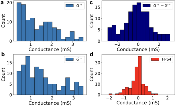
The image presents four histograms displaying conductance distributions. Each histogram represents a different condition or group: G+, G-, G+ - G-, and FP64. The x-axis of each histogram represents conductance in milliSiemens (mS), while the y-axis represents the count or frequency.
### Components/Axes
* **X-axis (all histograms):** Conductance (mS). Scale ranges from approximately -2 mS to 3 mS, varying slightly between plots.
* **Y-axis (all histograms):** Count. Scale ranges from 0 to approximately 30.
* **Histogram a:** Labelled "G+". Color: Blue. Legend is in the top-right corner.
* **Histogram b:** Labelled "G-". Color: Blue. Legend is in the top-right corner.
* **Histogram c:** Labelled "G+ - G-". Color: Dark Blue. Legend is in the top-right corner.
* **Histogram d:** Labelled "FP64". Color: Red. Legend is in the top-right corner.
### Detailed Analysis or Content Details
**Histogram a (G+):**
The distribution is unimodal, peaking at approximately 0.8 mS. The conductance values range from approximately 0.6 mS to 3.2 mS.
* Approximate counts:
* 0.6-0.8 mS: ~18
* 0.8-1.0 mS: ~12
* 1.0-1.2 mS: ~10
* 1.2-1.4 mS: ~8
* 1.4-1.6 mS: ~6
* 1.6-1.8 mS: ~5
* 1.8-2.0 mS: ~4
* 2.0-2.2 mS: ~3
* 2.2-2.4 mS: ~2
* 2.4-2.6 mS: ~1
* 2.6-2.8 mS: ~1
* 2.8-3.0 mS: ~1
* 3.0-3.2 mS: ~1
**Histogram b (G-):**
The distribution is unimodal, peaking at approximately 1.2 mS. The conductance values range from approximately 0.6 mS to 3.2 mS.
* Approximate counts:
* 0.6-0.8 mS: ~15
* 0.8-1.0 mS: ~13
* 1.0-1.2 mS: ~10
* 1.2-1.4 mS: ~8
* 1.4-1.6 mS: ~6
* 1.6-1.8 mS: ~5
* 1.8-2.0 mS: ~4
* 2.0-2.2 mS: ~3
* 2.2-2.4 mS: ~2
* 2.4-2.6 mS: ~2
* 2.6-2.8 mS: ~1
* 2.8-3.0 mS: ~1
* 3.0-3.2 mS: ~1
**Histogram c (G+ - G-):**
The distribution is approximately symmetrical and unimodal, peaking at approximately 0.2 mS. The conductance values range from approximately -2 mS to 2.2 mS.
* Approximate counts:
* -2.0 to -1.8 mS: ~5
* -1.8 to -1.6 mS: ~6
* -1.6 to -1.4 mS: ~7
* -1.4 to -1.2 mS: ~8
* -1.2 to -1.0 mS: ~9
* -1.0 to -0.8 mS: ~10
* -0.8 to -0.6 mS: ~11
* -0.6 to -0.4 mS: ~12
* -0.4 to -0.2 mS: ~13
* -0.2 to 0.0 mS: ~15
* 0.0 to 0.2 mS: ~14
* 0.2 to 0.4 mS: ~12
* 0.4 to 0.6 mS: ~10
* 0.6 to 0.8 mS: ~8
* 0.8 to 1.0 mS: ~6
* 1.0 to 1.2 mS: ~5
* 1.2 to 1.4 mS: ~4
* 1.4 to 1.6 mS: ~3
* 1.6 to 1.8 mS: ~2
* 1.8 to 2.0 mS: ~1
* 2.0 to 2.2 mS: ~1
**Histogram d (FP64):**
The distribution is unimodal, peaking at approximately 0.6 mS. The conductance values range from approximately -1.8 mS to 1.8 mS.
* Approximate counts:
* -1.8 to -1.6 mS: ~5
* -1.6 to -1.4 mS: ~8
* -1.4 to -1.2 mS: ~12
* -1.2 to -1.0 mS: ~16
* -1.0 to -0.8 mS: ~20
* -0.8 to -0.6 mS: ~24
* -0.6 to -0.4 mS: ~28
* -0.4 to -0.2 mS: ~30
* -0.2 to 0.0 mS: ~28
* 0.0 to 0.2 mS: ~24
* 0.2 to 0.4 mS: ~20
* 0.4 to 0.6 mS: ~16
* 0.6 to 0.8 mS: ~12
* 0.8 to 1.0 mS: ~8
* 1.0 to 1.2 mS: ~5
* 1.2 to 1.4 mS: ~3
* 1.4 to 1.6 mS: ~2
* 1.6 to 1.8 mS: ~1
### Key Observations
* The G+ and G- distributions are similar in shape, both being unimodal and skewed towards higher conductance values.
* The G+ - G- distribution is centered around zero, indicating a balanced difference between the G+ and G- conductance values.
* The FP64 distribution is also unimodal, but it is more narrowly distributed around a lower conductance value compared to G+ and G-.
* The FP64 distribution shows a much higher peak count (~30) than the other distributions.
### Interpretation
The data suggests that the conductance values for G+ and G- are distributed differently, with G+ generally exhibiting higher conductance. The G+ - G- distribution represents the difference in conductance between these two groups, and its centering around zero suggests a balance or cancellation of conductance effects. The FP64 distribution, with its distinct peak and narrower spread, likely represents a different population or condition with a characteristic conductance value. The higher peak in FP64 suggests a greater concentration of events around that specific conductance level. The differences in distributions could indicate varying mechanisms or properties underlying the conductance in each group. Further analysis would be needed to determine the biological or physical significance of these differences.