# Technical Data Extraction: Control Effect Analysis in LLMs
This document provides a comprehensive extraction of the data and trends presented in the provided multi-panel scientific figure. The figure analyzes the "Control effect (d)" across different models, layers, and principal components (PCs).
---
## Panel A: Score Distribution Histograms
**Type:** Frequency Histograms (Two sub-plots)
**Language:** English
### Sub-plot 1 (Left)
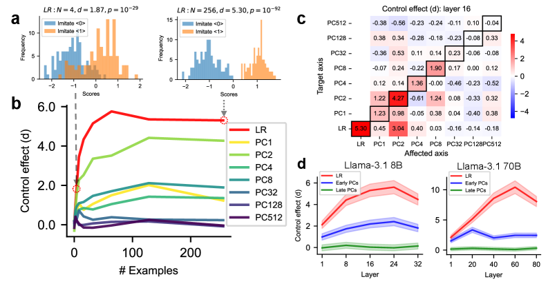
* **Header Text:** $LR : N = 4, d = 1.87, p = 10^{-29}$
* **Y-Axis:** Frequency (Scale: 0 to 10)
* **X-Axis:** Scores (Scale: -2 to 2)
* **Legend:**
* Blue: `Imitate <0>`
* Orange: `Imitate <1>`
* **Trend:** Two overlapping distributions. `Imitate <0>` centers around -1.0, while `Imitate <1>` centers around +0.8. The low $N$ (4) results in a lower effect size ($d=1.87$).
### Sub-plot 2 (Right)
* **Header Text:** $LR : N = 256, d = 5.30, p = 10^{-92}$
* **Y-Axis:** Frequency (Scale: 0 to 15)
* **X-Axis:** Scores (Scale: -2 to 2)
* **Legend:**
* Blue: `Imitate <0>`
* Orange: `Imitate <1>`
* **Trend:** Two distinct, non-overlapping distributions. `Imitate <0>` is tightly clustered around -1.0; `Imitate <1>` is tightly clustered around +1.2. The high $N$ (256) results in a very high effect size ($d=5.30$).
---
## Panel B: Control Effect vs. Number of Examples
**Type:** Line Graph
**Y-Axis:** Control effect (d) [Scale: 0.0 to 6.0]
**X-Axis:** # Examples [Scale: 0 to 200+]
### Data Series Extraction
| Series Label | Color | Visual Trend | Final Value (approx. N=256) |
| :--- | :--- | :--- | :--- |
| **LR** | Red | Rapid logarithmic growth, plateaus at high value. | ~5.3 |
| **PC1** | Yellow | Steady growth, plateaus. | ~4.2 |
| **PC2** | Light Green | Moderate growth, plateaus. | ~1.5 |
| **PC4** | Teal | Low growth, plateaus. | ~1.9 |
| **PC8** | Blue-Green | Low growth, plateaus. | ~1.3 |
| **PC32** | Blue | Initial spike, then declines to near zero. | ~0.2 |
| **PC128** | Dark Blue | Flat/Near zero. | ~0.0 |
| **PC512** | Purple | Flat/Near zero. | ~0.0 |
**Annotations:**
* A dashed vertical line at $N=4$ connects to the first histogram in Panel A.
* A dashed arrow at $N=256$ connects to the second histogram in Panel A.
---
## Panel C: Control Effect Heatmap (Layer 16)
**Type:** Heatmap Matrix
**Title:** Control effect (d): layer 16
**Y-Axis (Target axis):** PC512, PC128, PC32, PC8, PC4, PC2, PC1, LR
**X-Axis (Affected axis):** LR, PC1, PC2, PC4, PC8, PC32, PC128, PC512
**Color Scale:** Blue (-4) to White (0) to Red (+4)
### Matrix Values (Transcribed)
| Target \ Affected | LR | PC1 | PC2 | PC4 | PC8 | PC32 | PC128 | PC512 |
| :--- | :--- | :--- | :--- | :--- | :--- | :--- | :--- | :--- |
| **PC512** | -0.38 | -0.56 | -0.23 | -0.24 | -0.11 | 0.10 | -0.04 | **-0.04** |
| **PC128** | 0.38 | 0.34 | -0.28 | -0.18 | -0.23 | -0.08 | **0.33** | |
| **PC32** | -0.36 | 0.53 | 0.11 | 0.14 | 0.23 | **-0.06** | -0.08 | |
| **PC8** | -0.07 | 0.24 | -0.22 | **1.90** | 0.17 | 0.00 | 0.12 | |
| **PC4** | 0.12 | 0.14 | **1.36** | -0.00 | -0.46 | -0.23 | -0.52 | |
| **PC2** | 1.22 | **4.27** | -0.61 | 1.24 | 0.08 | -0.33 | 0.32 | |
| **PC1** | **1.23** | 0.98 | -0.05 | 0.38 | 0.04 | -0.40 | 0.38 | |
| **LR** | **5.30** | 0.45 | 3.04 | 0.40 | 0.03 | -0.16 | -0.14 | -0.18 |
*Note: Bolded boxes in the image indicate the diagonal/primary relationships.*
---
## Panel D: Control Effect across Layers
**Type:** Line Graphs with Shaded Error Bars (Two sub-plots)
**Y-Axis:** Control effect (d)
**X-Axis:** Layer
### Sub-plot 1: Llama-3.1 8B
* **X-Axis Range:** 1 to 32
* **Trends:**
* **LR (Red):** Increases steadily, peaks around layer 24 (d ≈ 5.5), then slightly declines.
* **Early PCs (Blue):** Increases to layer 24 (d ≈ 2.5), then declines.
* **Late PCs (Green):** Remains flat near zero across all layers.
### Sub-plot 2: Llama-3.1 70B
* **X-Axis Range:** 1 to 80
* **Trends:**
* **LR (Red):** Sharp increase, peaks around layer 60 (d ≈ 10.5), then declines.
* **Early PCs (Blue):** Peaks early (layer 20, d ≈ 4), drops, then plateaus around d ≈ 3.
* **Late PCs (Green):** Remains flat near zero across all layers.
---
**Summary of Findings:** The "LR" (Linear Regression) method consistently yields the highest control effect across different sample sizes and model scales, particularly in middle-to-late layers. Early Principal Components (PCs) show moderate effects, while late PCs show negligible control effects.