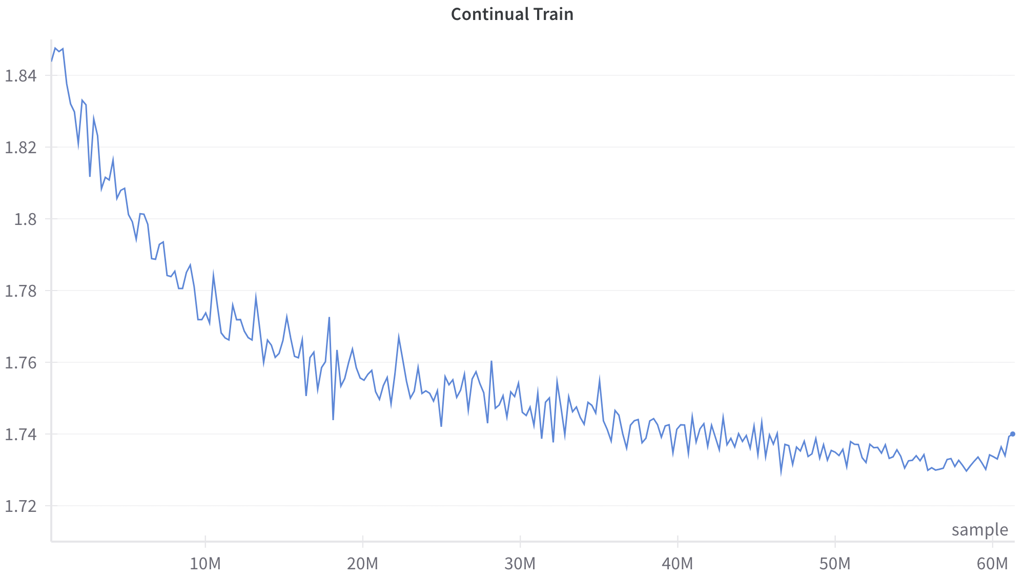
\n ## Line Chart: Continual Train ### Overview The image displays a line chart titled "Continual Train," plotting a single data series over a large number of samples. The chart shows a generally decreasing trend with significant high-frequency noise or volatility throughout the entire range. The visual suggests a metric (likely a loss or error rate) being tracked during a prolonged training process. ### Components/Axes * **Chart Title:** "Continual Train" (centered at the top). * **X-Axis:** * **Label:** "sample" (positioned at the bottom-right corner of the axis). * **Scale:** Linear scale from 0 to 60 million (60M) samples. * **Major Tick Marks:** Labeled at 10M, 20M, 30M, 40M, 50M, and 60M. * **Y-Axis:** * **Label:** No explicit axis title is present. * **Scale:** Linear scale ranging from approximately 1.72 to 1.85. * **Major Tick Marks:** Labeled at 1.72, 1.74, 1.76, 1.78, 1.80, 1.82, and 1.84. * **Data Series:** A single, continuous blue line. There is no legend, as only one series is plotted. ### Detailed Analysis **Trend Verification:** The blue line exhibits a clear, overall downward slope from left to right, indicating a decreasing value over the sample count. The trend is not smooth; it is characterized by constant, sharp fluctuations (noise) superimposed on the primary downward trajectory. **Data Point Extraction (Approximate):** * **Start (≈0 samples):** The line begins at its highest point, approximately **1.85**. * **10M Samples:** The value has dropped significantly to approximately **1.78**. The descent is steepest in this initial segment. * **20M Samples:** The value is approximately **1.76**. The rate of decrease has slowed compared to the first 10M samples. * **30M Samples:** The value is approximately **1.745**. The trend continues to flatten. * **40M Samples:** The value is approximately **1.735**. The line begins to show signs of plateauing. * **50M Samples:** The value is approximately **1.73**. The trend is largely flat with continued noise. * **60M Samples (End):** The line ends at a point slightly above the 1.74 grid line, approximately **1.74**. There is a very slight upward tick in the final few data points. **Noise Characterization:** The volatility is present across the entire x-axis. The amplitude of the fluctuations appears relatively consistent, spanning roughly ±0.01 to ±0.015 units on the y-axis, even as the mean value decreases. ### Key Observations 1. **Two-Phase Descent:** The chart shows a rapid initial improvement (steep negative slope) for the first ~15-20M samples, followed by a phase of diminishing returns where the improvement slows considerably. 2. **Convergence/Plateau:** After approximately 40M samples, the metric appears to stabilize or converge, oscillating within a narrow band between ~1.73 and ~1.74. 3. **Persistent Noise:** The training process exhibits significant and persistent variance at every stage, never producing a smooth curve. This suggests inherent noise in the optimization process or the data itself. 4. **Final Uptick:** There is a minor but noticeable upward movement in the very last segment of the line (approaching 60M samples), which could indicate the beginning of overfitting or simply noise at the end of the recorded data. ### Interpretation This chart almost certainly visualizes a **training loss curve** from a machine learning model undergoing continual or extended training. The y-axis, though unlabeled, represents a loss value (e.g., cross-entropy loss) that the model is minimizing. * **What it demonstrates:** The model is successfully learning, as evidenced by the consistent reduction in loss over 60 million training samples. The steep initial drop shows rapid early learning, while the later plateau indicates the model is approaching its performance limit on the given task/data. * **Relationship between elements:** The x-axis (samples) is the measure of training effort or exposure to data. The y-axis (loss) is the measure of model error. The downward trend confirms the training process is effective. * **Notable anomalies:** The persistent high-frequency noise is the most striking feature. In a typical training curve, one might expect a smoother line after smoothing or averaging. The raw, noisy plot suggests this is an unfiltered, per-batch or per-step loss value. The slight uptick at 60M samples warrants monitoring; if it continues, it could signal that further training is becoming detrimental. * **Underlying message:** The process requires a vast amount of data (60M samples) for convergence, and the final performance gain after the first 20M samples is relatively marginal. This highlights the computational cost of achieving the last few percentage points of improvement in model training.