\n
## Diagram: Variational Router Architecture
### Overview
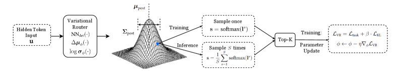
The image depicts a diagram of a Variational Router architecture, illustrating the flow of information from a Hidden Token Input through a Variational Router, a posterior distribution, sampling processes (during training and inference), and finally to a Top-K parameter update stage. The diagram highlights the mathematical operations involved in each step.
### Components/Axes
The diagram consists of the following components, arranged from left to right:
1. **Hidden Token Input (u):** The initial input to the system.
2. **Variational Router:** A neural network (NN) that takes the input 'u' and outputs Δμ(⋅), log σ(⋅).
3. **Posterior Distribution:** Represented as a 3D Gaussian surface, labeled with Σ<sub>post</sub> and μ<sub>post</sub>.
4. **Training Branch:** Indicates sampling once using s = softmax(Γ').
5. **Inference Branch:** Indicates sampling 's' times using s = Σ<sub>s=1</sub><sup>s</sup> softmax(Γ').
6. **Top-K:** A component for parameter update.
7. **Training Loss:** A box containing the equations for the loss function and parameter update.
### Detailed Analysis or Content Details
* **Hidden Token Input (u):** Labeled simply as "Hidden Token Input u".
* **Variational Router:** The router is described as NN<sub>φ</sub>(⋅), with outputs Δμ(⋅) and log σ(⋅). The φ likely represents the parameters of the neural network.
* **Posterior Distribution:** The posterior distribution is characterized by Σ<sub>post</sub> (covariance matrix) and μ<sub>post</sub> (mean vector). The 3D surface visually represents a Gaussian distribution.
* **Training Branch:** The training branch involves sampling once, where 's' is calculated as softmax(Γ'). Γ' is not further defined.
* **Inference Branch:** The inference branch involves sampling 's' times, where 's' is calculated as the sum of softmax(Γ') from s=1 to s.
* **Top-K:** This component is labeled "Top-K Parameter Update".
* **Training Loss:** The training loss is defined by the following equations:
* L<sub>VR</sub> = L<sub>data</sub> + λ L<sub>KL</sub>
* φ ← φ - η ∇<sub>φ</sub>L<sub>VR</sub>
Where:
* L<sub>VR</sub> is the Variational Router loss.
* L<sub>data</sub> is the data loss.
* L<sub>KL</sub> is the KL divergence loss.
* λ is a weighting factor.
* φ represents the parameters of the network.
* η is the learning rate.
* ∇<sub>φ</sub>L<sub>VR</sub> is the gradient of the loss with respect to the parameters.
### Key Observations
The diagram illustrates a variational inference approach. The Variational Router aims to approximate the posterior distribution. The training process involves minimizing a loss function that balances data fit (L<sub>data</sub>) and the KL divergence between the approximate posterior and the true posterior (L<sub>KL</sub>). The Top-K component suggests a method for selecting the most important parameters for updating.
### Interpretation
This diagram represents a novel approach to routing information within a neural network using variational inference. The Variational Router learns a posterior distribution over possible routes, allowing for more flexible and robust information flow. The use of a variational approach introduces uncertainty into the routing process, which can be beneficial for generalization and exploration. The Top-K parameter update suggests a method for focusing on the most important parameters during training, potentially improving efficiency and performance. The diagram highlights the mathematical foundations of the architecture, emphasizing the use of Gaussian distributions, softmax functions, and gradient-based optimization. The separation of training and inference branches indicates different sampling strategies are employed in each phase. The overall architecture appears designed to address challenges in complex neural networks where traditional routing methods may be insufficient.