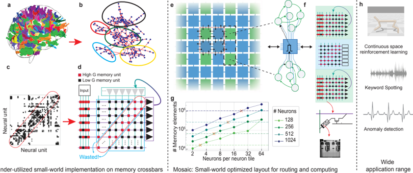
\n ## Diagram: Neuromorphic Computing Architecture ### Overview This diagram illustrates a neuromorphic computing architecture, focusing on a small-world network implementation on memory crossbars and a mosaic layout optimized for routing and computing. It showcases the transition from a complex network to a simplified representation, the structure of memory units, and the application of this architecture to various tasks. ### Components/Axes The diagram is segmented into several parts: * **(a)**: A complex, colorful network representation. * **(b)**: A simplified network representation with nodes and connections. A circle highlights a specific region. * **(c)**: A scatter plot showing neural unit activity. X-axis labeled "Neural unit", Y-axis labeled "Neural unit". * **(d)**: A grid representing a memory unit, with "High G memory unit" (red squares) and "Low G memory unit" (black squares). Labeled "Input" points to the top row. "Wasted" is labeled at the bottom right. * **(e)**: A mosaic layout of interconnected tiles. * **(f)**: A schematic showing connections between tiles and memory units, with a symbol resembling a resistor (Ω) in the center. * **(g)**: A log-log plot of "# Memory elements" vs. "# Neurons per neuron tile". X-axis ranges from 2 to 64. Y-axis ranges from 10^0 to 10^6. * **(h)**: Illustrations of applications: Continuous space reinforcement learning, Keyword Spotting, and Anomaly detection. * **Footer**: Text describing the architecture: "Under-utilized small-world implementation on memory crossbars" and "Mosaic: Small-world optimized layout for routing and computing". ### Detailed Analysis or Content Details **Part (a) & (b): Network Simplification** Part (a) shows a highly interconnected network with nodes colored in various shades (red, green, blue, purple). Part (b) presents a simplified view of the same network, with nodes represented as dots (purple and green) and connections as lines. The highlighted circle in (b) suggests a focus on a specific sub-network. **Part (c): Neural Unit Activity** This is a scatter plot showing the activity of neural units. The plot appears to have a sparse distribution of points, indicating that not all neural units are active simultaneously. The density of points is relatively low. **Part (d): Memory Unit Structure** The grid represents a memory unit. Red squares denote "High G memory unit", while black squares denote "Low G memory unit". The "Input" is at the top. The bottom right corner is labeled "Wasted", suggesting unused memory space. The grid is approximately 10x10. **Part (e): Mosaic Layout** This shows a grid of interconnected tiles. Each tile contains a smaller grid of units. The tiles are connected, forming a larger network. **Part (f): Tile Connections** This schematic illustrates how tiles are connected to memory units. The resistor symbol (Ω) likely represents a weighting or resistance value in the circuit. The connections appear to be bidirectional. **Part (g): Memory Elements vs. Neurons** This log-log plot shows the relationship between the number of memory elements and the number of neurons per neuron tile. There are five lines representing different numbers of neurons: 128 (dark green), 256 (blue), 512 (light green), 1024 (red), and a dashed line representing a theoretical limit. * **128 Neurons (Dark Green):** Starts at approximately 10^3 memory elements at 2 neurons/tile, and rises to approximately 2x10^5 memory elements at 64 neurons/tile. * **256 Neurons (Blue):** Starts at approximately 2x10^3 memory elements at 2 neurons/tile, and rises to approximately 4x10^5 memory elements at 64 neurons/tile. * **512 Neurons (Light Green):** Starts at approximately 4x10^3 memory elements at 2 neurons/tile, and rises to approximately 8x10^5 memory elements at 64 neurons/tile. * **1024 Neurons (Red):** Starts at approximately 8x10^3 memory elements at 2 neurons/tile, and rises to approximately 1.6x10^6 memory elements at 64 neurons/tile. * **Dashed Line:** Represents a theoretical upper bound, starting at approximately 1x10^3 memory elements at 2 neurons/tile, and rising to approximately 1x10^6 memory elements at 64 neurons/tile. All lines exhibit a positive slope, indicating that the number of memory elements increases with the number of neurons per tile. The lines are roughly parallel, suggesting a linear relationship. **Part (h): Applications** This section demonstrates the application of the architecture to three tasks: * **Continuous space reinforcement learning:** Shown with a waveform. * **Keyword Spotting:** Shown with a waveform. * **Anomaly detection:** Shown with a waveform. A small image of a chip is also shown with an arrow pointing to "Wide application range". ### Key Observations * The architecture leverages a small-world network for efficient routing and computation. * The memory unit structure utilizes both high and low conductance memory units. * The number of memory elements scales with the number of neurons per tile, but there appears to be a limit to this scaling. * The architecture is versatile and can be applied to various machine learning tasks. ### Interpretation The diagram presents a novel neuromorphic computing architecture that aims to overcome the limitations of traditional von Neumann architectures. The small-world network implementation on memory crossbars provides efficient routing and computation, while the mosaic layout allows for scalability. The use of both high and low conductance memory units enables more complex computations. The log-log plot (g) suggests a trade-off between the number of memory elements and the number of neurons per tile, indicating that there is a limit to how densely the network can be packed. The applications shown in (h) demonstrate the potential of this architecture for a wide range of machine learning tasks. The "Wasted" label in (d) suggests that there is room for optimization in the memory unit design. The overall design appears to be focused on energy efficiency and parallel processing, which are key advantages of neuromorphic computing.