TECHNICAL ASSET FINGERPRINT
0b6ec1aa43fa69ca8a0e704c
Click to view fullscreen
Press ESC or click to close
FOUND IN PAPERS
EXPERT: healer-alpha-free VERSION 1
RUNTIME: free/openrouter/healer-alpha
INTEL_VERIFIED
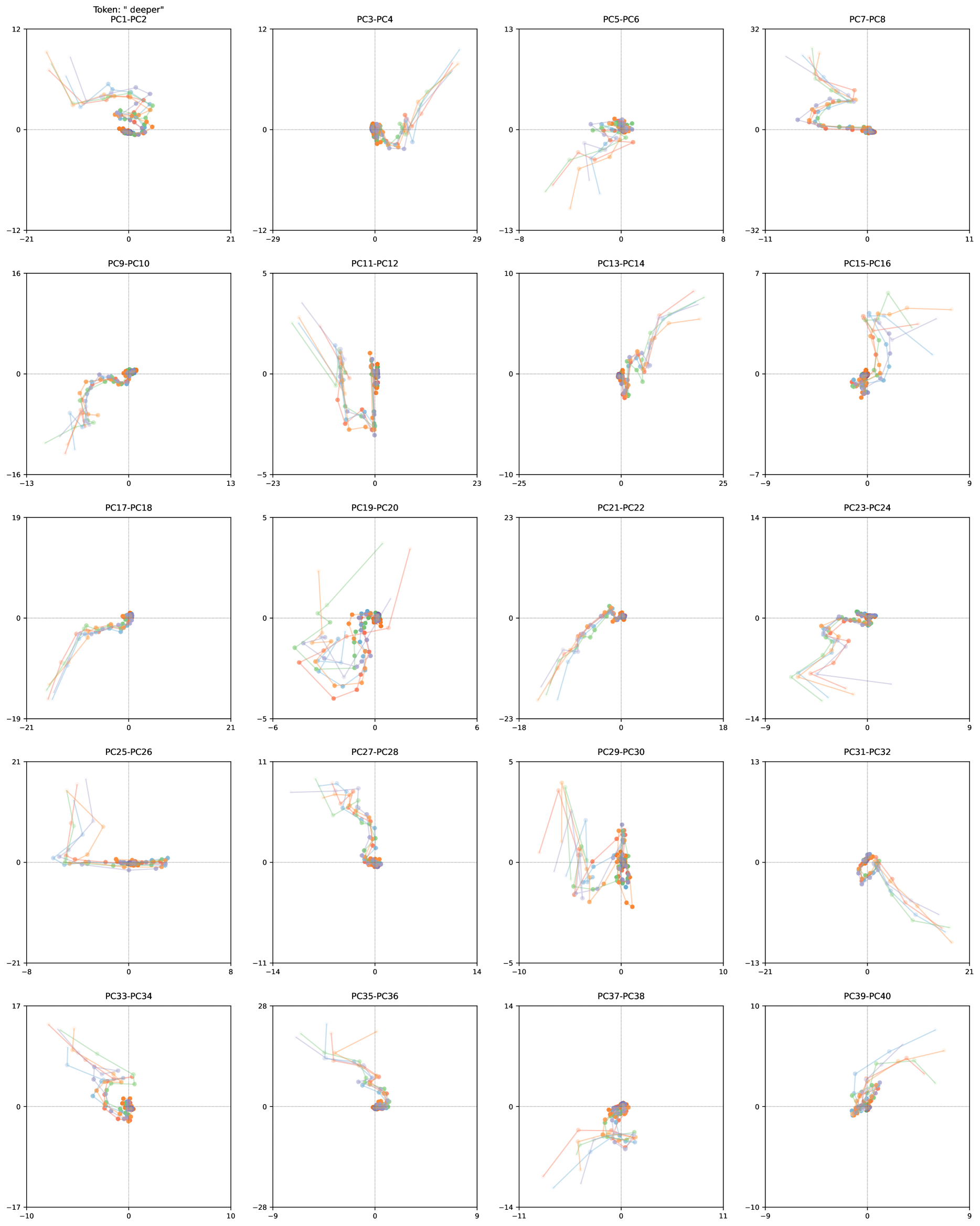
## Scatter Plot Matrix: Principal Component Projections for Token "deeper"
### Overview
The image displays a 5x4 grid of 20 scatter plots. Each plot visualizes the relationship between a pair of Principal Components (PCs) for the token "deeper". The data points are connected by lines, forming trajectories, and are colored in multiple distinct hues (orange, green, blue, purple, etc.), suggesting different categories or sequences. There is no legend provided to identify what these colors represent. The overall purpose appears to be analyzing the variance and structure of the token's representation across different principal component dimensions.
### Components/Axes
* **Global Title:** Located at the top-left corner: `Token: " deeper"`.
* **Subplot Titles:** Each of the 20 subplots has a title indicating the PC pair being plotted (e.g., `PC1-PC2`, `PC3-PC4`, ..., `PC39-PC40`).
* **Axes:** Each subplot has an x-axis and a y-axis. The axes are labeled with numerical tick marks but lack descriptive titles (e.g., "Principal Component 1"). The ranges vary significantly between plots.
* **Data Series:** Each plot contains multiple series, distinguished by color (orange, green, light blue, purple, etc.). Each series is a connected scatter plot, showing a trajectory of points.
* **Grid Layout:** The plots are arranged in a uniform grid with 5 rows and 4 columns.
### Detailed Analysis
The following table details the title and axis ranges for each subplot, proceeding row by row from top-left to bottom-right.
| Position (Row, Col) | Subplot Title | X-Axis Range (Approx.) | Y-Axis Range (Approx.) | Visual Trend Description |
| :--- | :--- | :--- | :--- | :--- |
| (1,1) | PC1-PC2 | -21 to 21 | -12 to 12 | Multiple colored trajectories converge from the top-left quadrant towards a dense cluster near the origin (0,0). |
| (1,2) | PC3-PC4 | -29 to 29 | -12 to 12 | Trajectories start near the origin and fan out upwards and to the right into the first quadrant. |
| (1,3) | PC5-PC6 | -8 to 8 | -13 to 13 | Trajectories are tightly clustered near the origin, with some lines extending into the third quadrant (bottom-left). |
| (1,4) | PC7-PC8 | -11 to 11 | -32 to 32 | Trajectories form a loose cluster near the origin, with some lines extending into the second quadrant (top-left). |
| (2,1) | PC9-PC10 | -13 to 13 | -16 to 16 | Trajectories form a curved path from the third quadrant (bottom-left) up towards the origin. |
| (2,2) | PC11-PC12 | -23 to 23 | -5 to 5 | Trajectories are vertically oriented, clustered along the y-axis near x=0, spanning from negative to positive y-values. |
| (2,3) | PC13-PC14 | -25 to 25 | -10 to 10 | Trajectories start near the origin and extend diagonally upwards into the first quadrant. |
| (2,4) | PC15-PC16 | -9 to 9 | -7 to 7 | A dense, tangled cluster of trajectories centered near the origin. |
| (3,1) | PC17-PC18 | -21 to 21 | -19 to 19 | Trajectories form a curved path from the third quadrant up towards the origin. |
| (3,2) | PC19-PC20 | -6 to 6 | -5 to 5 | A complex, tangled web of trajectories centered near the origin, with some lines extending into all quadrants. |
| (3,3) | PC21-PC22 | -18 to 18 | -23 to 23 | Trajectories form a diagonal line from the third quadrant to the first quadrant, passing through the origin. |
| (3,4) | PC23-PC24 | -14 to 14 | -9 to 9 | Trajectories form a loose, horizontal cluster near y=0, spanning the x-axis. |
| (4,1) | PC25-PC26 | -8 to 8 | -21 to 21 | Trajectories form a horizontal cluster near y=0, with some lines extending vertically upwards. |
| (4,2) | PC27-PC28 | -14 to 14 | -11 to 11 | Trajectories are vertically oriented, clustered along the y-axis near x=0. |
| (4,3) | PC29-PC30 | -10 to 10 | -5 to 5 | A dense, vertical cluster of trajectories centered near x=0. |
| (4,4) | PC31-PC32 | -21 to 21 | -13 to 13 | Trajectories form a diagonal line from the origin down into the fourth quadrant (bottom-right). |
| (5,1) | PC33-PC34 | -10 to 10 | -17 to 17 | Trajectories form a curved path from the second quadrant (top-left) down towards the origin. |
| (5,2) | PC35-PC36 | -9 to 9 | -28 to 28 | Trajectories form a diagonal line from the second quadrant down to the origin. |
| (5,3) | PC37-PC38 | -11 to 11 | -14 to 14 | A dense cluster of trajectories centered near the origin. |
| (5,4) | PC39-PC40 | -9 to 9 | -10 to 10 | Trajectories start near the origin and extend diagonally upwards into the first quadrant. |
### Key Observations
1. **Varying Structure:** The relationship between token embeddings changes dramatically across different PC pairs. Some show tight clusters (e.g., PC15-PC16), others show clear linear trends (e.g., PC21-PC22), and others show complex, non-linear trajectories (e.g., PC19-PC20).
2. **Central Tendency:** The origin (0,0) is a strong focal point in nearly all plots, with most data trajectories converging to or passing through it.
3. **Color-Coded Trajectories:** The use of multiple colors implies the data is grouped into several distinct series (e.g., different contexts, layers, or attention heads). However, the **critical missing information** is a legend to decode these colors.
4. **Axis Scale Disparity:** The numerical ranges on the axes differ greatly between plots (e.g., PC7-PC8 y-axis spans 64 units, while PC29-PC30 y-axis spans only 10 units), indicating that the variance captured by each principal component pair is not uniform.
### Interpretation
This visualization is a diagnostic tool for understanding the internal representation of the token "deeper" within a machine learning model, likely a transformer-based language model. Principal Component Analysis (PCA) has been used to reduce the high-dimensional embedding space into 2D projections.
* **What it demonstrates:** The plots reveal that the token's representation is not a single point but a structured manifold. The different colored lines likely trace the token's representation through different layers of the model or across different contextual examples. The convergence to the origin in many plots suggests that after PCA transformation, the mean of the data is centered at zero.
* **Relationships between elements:** The grid allows comparison of how the token's variance is distributed across orthogonal directions (the PCs). Early PCs (e.g., PC1-PC4) often capture the most significant variance, which is visible here as broader spreads. Later PCs show more nuanced or noise-related structure.
* **Notable anomalies/patterns:** The stark difference in structure between adjacent plots (e.g., the vertical line in PC11-PC12 vs. the diagonal in PC13-PC14) highlights that the principal components are capturing fundamentally different aspects of the data's variation. The lack of a legend is a significant limitation, preventing the viewer from attributing the observed trajectories to specific model components or contexts, which is essential for a full technical interpretation.
DECODING INTELLIGENCE...