## Line Graphs: ViSQOL vs. Bitrate Across Different Conditions
### Overview
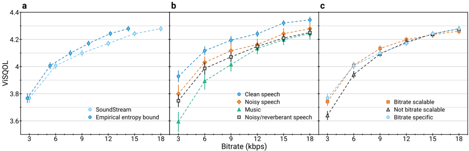
The image contains three subplots (a, b, c) comparing ViSQOL scores against bitrate (3–18 kbps) for various audio conditions. Each subplot uses distinct data series and legends to represent different scenarios.
---
### Components/Axes
- **X-axis**: Bitrate (kbps), ranging from 3 to 18 kbps in increments of 3.
- **Y-axis**: ViSQOL score, ranging from 3.6 to 4.4.
- **Legends**:
- **Subplot a**:
- Dashed blue line with circles: **SoundStream**
- Solid blue line with diamonds: **Empirical entropy bound**
- **Subplot b**:
- Blue circles: **Clean speech**
- Orange diamonds: **Noisy speech**
- Green triangles: **Music**
- Black squares: **Noisy/reverberant speech**
- **Subplot c**:
- Orange diamonds: **Bitrate scalable**
- Black triangles: **Not bitrate scalable**
- Blue circles: **Bitrate specific**
---
### Detailed Analysis
#### Subplot a
- **Trend**: Both lines show a consistent upward trend. The dashed line (SoundStream) starts slightly below the solid line (Empirical entropy bound) but converges near 18 kbps.
- **Data Points**:
- At 3 kbps: SoundStream ≈ 3.78, Empirical entropy bound ≈ 3.78.
- At 18 kbps: SoundStream ≈ 4.28, Empirical entropy bound ≈ 4.30.
#### Subplot b
- **Trend**: All series increase with bitrate, but starting points and growth rates vary.
- **Clean speech**: Steady rise from ~3.9 to ~4.3.
- **Noisy speech**: Starts lower (~3.8) but grows to ~4.2.
- **Music**: Starts lowest (~3.6) but rises steeply to ~4.1.
- **Noisy/reverberant speech**: Moderate growth from ~3.7 to ~4.2.
- **Data Points**:
- At 3 kbps: Clean speech ≈ 3.9, Noisy speech ≈ 3.8, Music ≈ 3.6, Noisy/reverberant ≈ 3.7.
- At 18 kbps: Clean speech ≈ 4.35, Noisy speech ≈ 4.25, Music ≈ 4.15, Noisy/reverberant ≈ 4.2.
#### Subplot c
- **Trend**: All series increase, but "Bitrate scalable" and "Bitrate specific" outperform "Not bitrate scalable."
- **Bitrate scalable**: Starts at ~3.8, ends at ~4.3.
- **Not bitrate scalable**: Starts at ~3.7, ends at ~4.2.
- **Bitrate specific**: Starts at ~3.9, ends at ~4.3.
- **Data Points**:
- At 3 kbps: Bitrate scalable ≈ 3.8, Not bitrate scalable ≈ 3.7, Bitrate specific ≈ 3.9.
- At 18 kbps: Bitrate scalable ≈ 4.28, Not bitrate scalable ≈ 4.2, Bitrate specific ≈ 4.3.
---
### Key Observations
1. **Bitrate Correlation**: Higher bitrates consistently improve ViSQOL scores across all conditions.
2. **Content Type Impact**: Music (subplot b) shows the lowest initial ViSQOL but gains significantly with bitrate, suggesting sensitivity to compression artifacts.
3. **Scalability**: "Bitrate scalable" (subplot c) outperforms "Not bitrate scalable," indicating adaptive bitrate strategies enhance quality.
4. **Empirical Bound**: In subplot a, the "Empirical entropy bound" closely tracks the "SoundStream" line, suggesting it represents a theoretical upper limit for ViSQOL.
---
### Interpretation
The data demonstrates that **bitrate is a critical factor in audio quality**, with higher bitrates improving ViSQOL scores across diverse conditions. However, the **type of content** (e.g., music vs. speech) and **bitrate scalability** significantly influence performance. For instance:
- **Music** requires higher bitrates to achieve parity with speech, likely due to its complex frequency content.
- **Bitrate scalable** methods (subplot c) outperform fixed or non-scalable approaches, highlighting the value of adaptive bitrate allocation.
- The **Empirical entropy bound** in subplot a suggests a theoretical ceiling for ViSQOL, which practical systems like SoundStream approach but do not exceed.
These findings underscore the importance of optimizing bitrate allocation based on content type and system capabilities to maximize perceived audio quality.