\n
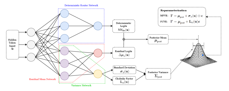
## Diagram: Neural Network Architecture for Variational Inference
### Overview
The image depicts a neural network architecture designed for variational inference. It illustrates the flow of information through a deterministic router network, a residual mean network, and a variance network, culminating in the reparameterization of a distribution. The diagram highlights the key components and their relationships in a probabilistic modeling context.
### Components/Axes
The diagram is segmented into three main sections: the input layer, the network layers (Deterministic Router Network, Residual Mean Network, Variance Network), and the reparameterization/output section.
* **Input:** "Hidden Token Input u"
* **Deterministic Router Network:** Labeled in blue.
* **Residual Mean Network:** Labeled in red.
* **Variance Network:** Labeled in green.
* **Outputs:**
* "Deterministic Logits NN<sub>det</sub>(u)"
* "Residual Logits Δμ<sub>det</sub>(u)"
* "Standard Deviation σ<sub>det</sub>(u)"
* "Cholesky Factor L<sub>σ</sub>(u)"
* **Reparameterisation:**
* "MFVR: I<sup>*</sup> = μ<sub>post</sub> + σ<sub>det</sub>(u)ε"
* "FCVR: I<sup>*</sup> = μ<sub>post</sub> + L<sub>σ</sub>(u)ε"
* **Posterior Distribution:** Visualized as a 3D cone-shaped surface.
* "Posterior Mean μ<sub>post</sub>"
* "Posterior Variance Σ<sub>post</sub>"
* **ε:** Represents a random variable.
### Detailed Analysis or Content Details
The diagram shows a neural network with multiple layers.
1. **Input Layer:** A single input node labeled "Hidden Token Input u".
2. **Deterministic Router Network (Blue):** This network consists of four layers of nodes. The input 'u' is connected to the first layer, which has four nodes. This layer is connected to a second layer with four nodes, then to a third layer with three nodes, and finally to an output layer with two nodes labeled "Deterministic Logits NN<sub>det</sub>(u)".
3. **Residual Mean Network (Red):** This network also has four layers of nodes. The input 'u' is connected to the first layer with four nodes, then to a second layer with four nodes, a third layer with three nodes, and finally to an output node labeled "Residual Logits Δμ<sub>det</sub>(u)".
4. **Variance Network (Green):** This network has four layers of nodes. The input 'u' is connected to the first layer with four nodes, then to a second layer with four nodes, a third layer with three nodes, and finally to two output nodes labeled "Standard Deviation σ<sub>det</sub>(u)" and "Cholesky Factor L<sub>σ</sub>(u)".
5. **Reparameterization:** The outputs from the networks are used in the reparameterization formulas for MFVR (Mean-Field Variational Representation) and FCVR (Fully-Connected Variational Representation). Both formulas involve adding a scaled random variable ε to a mean (μ<sub>post</sub>).
6. **Posterior Distribution:** The reparameterized output I<sup>*</sup> is used to define the posterior distribution, characterized by its mean (μ<sub>post</sub>) and variance (Σ<sub>post</sub>). The posterior distribution is visualized as a 3D cone-shaped surface.
### Key Observations
The diagram emphasizes the use of neural networks to model the posterior distribution in variational inference. The deterministic router network, residual mean network, and variance network work in parallel to estimate the parameters of the posterior distribution. The reparameterization trick is used to enable gradient-based optimization. The visualization of the posterior distribution as a cone suggests a unimodal distribution.
### Interpretation
This diagram illustrates a sophisticated approach to variational inference using neural networks. The architecture allows for flexible modeling of complex posterior distributions. The use of separate networks for the mean and variance components enables the model to capture dependencies between these parameters. The reparameterization trick is crucial for enabling gradient-based optimization, which is essential for training the neural networks. The diagram suggests a method for approximating intractable posterior distributions with a more tractable, parameterized form, allowing for efficient inference in Bayesian models. The separation of the deterministic router network suggests a mechanism for controlling the flow of information and potentially improving the accuracy of the approximation. The use of a Cholesky factor for the variance suggests a focus on maintaining positive definiteness, which is important for ensuring the validity of the posterior distribution. The diagram is a high-level overview of a complex system, and further details would be needed to fully understand its implementation and performance.