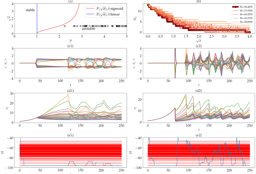
## Chart/Diagram Type: Multi-Panel Figure ### Overview The image is a multi-panel figure consisting of six subplots, arranged in a 3x2 grid. The subplots display various relationships between parameters, including stability analysis, population dynamics, and energy levels. The figure explores the behavior of a system under different conditions, likely related to a physical or biological model. ### Components/Axes **Panel (a): Stability Diagram** * **X-axis:** μ (mu), ranging from 0 to 5. * **Y-axis:** √a (square root of a), ranging from 0 to 4. * **Curves:** * Red line: F(√a), f sigmoid * Blue line: F(√a), f linear * **Regions:** * "stable" region to the left of the blue line (μ ≈ 1). * "unstable" region indicated by black 'x' marks to the right of the red line. **Panel (b): Population Dynamics** * **X-axis:** √a (square root of a), ranging from 0 to 4. * **Y-axis:** N_u, ranging from 0 to 12. * **Curves:** Multiple lines representing different values of H (energy), ranging from -96.4870 to -58.8590. The lines are colored in shades of brown, with darker shades representing lower H values. * H = -96.4870 (darkest brown) * H = -73.5530 * H = -69.2970 * H = -63.2750 * H = -58.8590 (lightest brown) **Panel (c1) and (c2): Time Series of <x_i>** * **X-axis:** t (time), ranging from 0 to 250. * **Y-axis:** <x_i>, ranging from -4 to 4. * **Curves:** Multiple lines, each representing a different instance or component of the system. **Panel (d1) and (d2): Time Series of e_i** * **X-axis:** t (time), ranging from 0 to 250. * **Y-axis:** e_i, ranging from 0 to 30. * **Curves:** Multiple lines, each representing a different instance or component of the system. **Panel (e1) and (e2): Time Series of H** * **X-axis:** t (time), ranging from 0 to 250. * **Y-axis:** H (energy), ranging from -100 to -40. * **Curves:** * Multiple red lines clustered around -60. * A single blue line showing fluctuations in energy. ### Detailed Analysis or ### Content Details **Panel (a): Stability Diagram** * The blue line (F(√a), f linear) is a vertical line at μ ≈ 1, indicating a sharp transition to instability. * The red line (F(√a), f sigmoid) curves upward, showing that the system becomes unstable at lower √a values as μ increases. * The region to the left of the blue line is labeled "stable," while the region to the right of the red line is marked with "x" symbols and labeled "unstable." **Panel (b): Population Dynamics** * The number of populations, N_u, decreases as √a increases. * The different H values (energy levels) influence the rate of decrease in N_u. Lower H values (darker brown lines) show a steeper decrease in N_u as √a increases. * The lines show a step-wise decrease, suggesting discrete population levels. **Panel (c1) and (c2): Time Series of <x_i>** * In panel (c1), the lines start at approximately 0 and then diverge around t=50, oscillating before settling to a value between -2 and 2. * In panel (c2), the lines start at approximately 0 and then diverge around t=50, oscillating with larger amplitudes than in (c1). **Panel (d1) and (d2): Time Series of e_i** * In both panels, the lines start at approximately 0 and then increase rapidly around t=50. * The lines in panel (d1) show a more gradual increase and then oscillate. * The lines in panel (d2) show a more rapid increase and larger oscillations. **Panel (e1) and (e2): Time Series of H** * In both panels, there are multiple red lines clustered around -60. * The blue line in panel (e1) shows a few drops in energy around t=125 and t=175. * The blue line in panel (e2) shows more frequent and larger fluctuations in energy. ### Key Observations * Panel (a) shows the stability of the system based on parameters μ and √a, with a clear distinction between stable and unstable regions. * Panel (b) illustrates how the population dynamics (N_u) are affected by √a and the energy level (H). * Panels (c1) and (c2) show the time evolution of <x_i> under two different conditions. * Panels (d1) and (d2) show the time evolution of e_i under two different conditions. * Panels (e1) and (e2) show the time evolution of H under two different conditions. ### Interpretation The figure presents a comprehensive analysis of a system's behavior, exploring its stability, population dynamics, and energy levels. The stability diagram in panel (a) defines the conditions under which the system remains stable or becomes unstable. Panel (b) shows how the population dynamics are influenced by the system's parameters. Panels (c), (d), and (e) show the time evolution of different variables under two different conditions, allowing for a comparison of the system's behavior. The differences between the left and right columns (c1/c2, d1/d2, e1/e2) likely represent different parameter settings or initial conditions, leading to distinct dynamic behaviors. The clustering of red lines in panels (e1) and (e2) suggests a common energy level, while the blue line indicates fluctuations or transitions in the system's energy state.