## Sequential Grid Transformation Diagram
### Overview
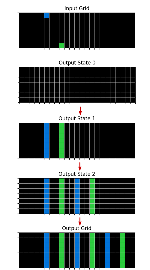
The image displays a five-step vertical sequence illustrating a transformation process on a grid-based system. It begins with an "Input Grid" containing two isolated colored cells and progresses through three intermediate states ("Output State 0", "Output State 1", "Output State 2") to a final "Output Grid". Red downward-pointing arrows connect each step, indicating the flow of the process. The visualization demonstrates a pattern of expansion and replication based on initial conditions.
### Components/Axes
* **Grid Structure:** Each step is represented by a rectangular grid of cells. The initial grids ("Input Grid" through "Output State 2") appear to have dimensions of approximately 10 rows by 20 columns. The final "Output Grid" is wider, with an estimated 10 rows by 30 columns.
* **Labels:** Each grid has a centered text label above it:
* "Input Grid"
* "Output State 0"
* "Output State 1"
* "Output State 2"
* "Output Grid"
* **Visual Elements:**
* **Cells:** The background of all grids is black, with a white grid line overlay defining individual cells.
* **Colors:** Two distinct colors are used for data representation: a medium blue and a medium green.
* **Arrows:** Solid red arrows point downward between the grids, connecting the bottom of one grid to the top of the next, establishing the sequence order.
### Detailed Analysis
The transformation process is analyzed step-by-step:
1. **Input Grid:**
* Contains two single, isolated colored cells.
* **Blue Cell:** Located in the top row (Row 1), approximately at Column 8 (counting from the left).
* **Green Cell:** Located in the bottom row (Row 10), approximately at Column 12.
2. **Output State 0:**
* The grid is entirely black. No colored cells are present. This represents a reset or initial blank state following the input.
3. **Output State 1:**
* Two full vertical columns are now colored.
* **Blue Column:** Column 8 is entirely filled with blue from Row 1 to Row 10.
* **Green Column:** Column 12 is entirely filled with green from Row 1 to Row 10.
* **Trend:** The initial single cells from the Input Grid have expanded vertically to fill their entire respective columns.
4. **Output State 2:**
* Four full vertical columns are colored, showing a replication pattern.
* **Blue Column 1:** Column 8 (blue).
* **Green Column 1:** Column 12 (green).
* **Blue Column 2:** Column 16 (blue).
* **Green Column 2:** Column 20 (green).
* **Trend:** The pattern from State 1 (a blue column followed 4 columns later by a green column) has been replicated once to the right. The new blue column is 4 columns right of the first green column, and the new green column is 4 columns right of that.
5. **Output Grid:**
* Six full vertical columns are colored, continuing the replication.
* **Blue Column 1:** Column 8 (blue).
* **Green Column 1:** Column 12 (green).
* **Blue Column 2:** Column 16 (blue).
* **Green Column 2:** Column 20 (green).
* **Blue Column 3:** Column 24 (blue).
* **Green Column 3:** Column 28 (green).
* **Trend:** The replication pattern has been applied a second time, adding another pair of blue and green columns, each spaced 4 columns apart, to the right side of the grid. The grid itself has expanded horizontally to accommodate these new columns.
### Key Observations
* **Pattern Rule:** The core rule appears to be: 1) Expand initial colored cells to fill their columns. 2) Replicate the resulting pattern (a blue column followed by a green column four columns to its right) iteratively to the right.
* **Fixed Spacing:** The horizontal spacing between the start of each colored column in the sequence is consistently 4 columns (e.g., from column 8 to 12, 12 to 16, etc.).
* **Color Order:** The sequence always maintains the order: Blue, Green, Blue, Green...
* **Grid Expansion:** The canvas (grid width) dynamically expands to the right to fit the growing pattern in the final output.
### Interpretation
This diagram visually encodes a deterministic, rule-based process, likely representing an algorithm or a cellular automaton. The process takes sparse input (two points) and generates a structured, periodic output through two clear phases: **vertical expansion** (filling columns) and **horizontal replication** (copying the column pattern with fixed spacing).
The data suggests a system where initial conditions trigger a cascade that fills defined channels (columns) and then propagates that structure in a predictable, repeating manner. This could model concepts in parallel computing (where a task spawns workers in a grid), pattern generation in procedural algorithms, or the behavior of a simple computational system where local rules lead to global order. The clear, step-by-step breakdown makes the underlying logic transparent, emphasizing how simple rules can lead to complex, expanding patterns.