\n
## Histograms: Price and Duration Distributions of o1-Mini
### Overview
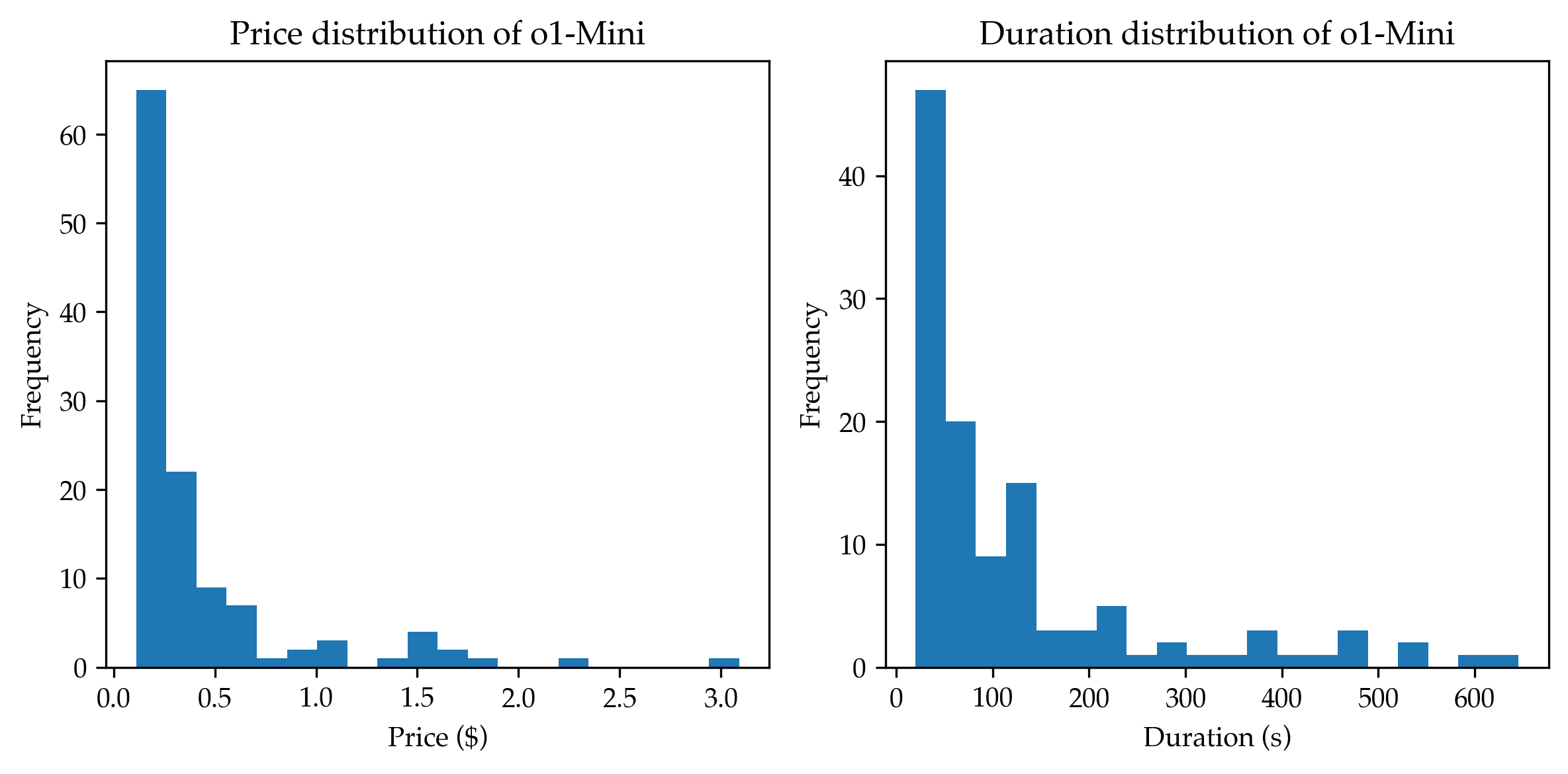
The image displays two side-by-side histograms presenting statistical distributions for a subject identified as "o1-Mini." The left chart shows the distribution of price in US dollars, and the right chart shows the distribution of duration in seconds. Both histograms are rendered in a standard blue color against a white background with black axes and labels. The data in both charts is heavily right-skewed.
### Components/Axes
**Left Histogram:**
* **Title:** "Price distribution of o1-Mini" (centered at the top).
* **X-axis:** Labeled "Price ($)". The axis has major tick marks and numerical labels at 0.0, 0.5, 1.0, 1.5, 2.0, 2.5, and 3.0.
* **Y-axis:** Labeled "Frequency". The axis has major tick marks and numerical labels at 0, 10, 20, 30, 40, 50, and 60.
**Right Histogram:**
* **Title:** "Duration distribution of o1-Mini" (centered at the top).
* **X-axis:** Labeled "Duration (s)". The axis has major tick marks and numerical labels at 0, 100, 200, 300, 400, 500, and 600.
* **Y-axis:** Labeled "Frequency". The axis has major tick marks and numerical labels at 0, 10, 20, 30, and 40.
**Spatial Grounding:** Both charts are of equal size, placed horizontally adjacent. Titles are positioned directly above their respective plot areas. Axis labels are centered below the x-axes and rotated 90 degrees to the left of the y-axes.
### Detailed Analysis
**Price Distribution (Left Chart):**
* **Trend Verification:** The distribution is strongly right-skewed (positively skewed). The frequency is highest for the lowest price bin and decreases rapidly as price increases, with a long, sparse tail extending to the right.
* **Data Points (Approximate Frequencies per Bin):**
* Bin 0.0 - ~0.25: Frequency ≈ 65 (the mode).
* Bin ~0.25 - 0.5: Frequency ≈ 22.
* Bin 0.5 - ~0.75: Frequency ≈ 9.
* Bin ~0.75 - 1.0: Frequency ≈ 7.
* Bin 1.0 - ~1.25: Frequency ≈ 1.
* Bin ~1.25 - 1.5: Frequency ≈ 2.
* Bin 1.5 - ~1.75: Frequency ≈ 3.
* Bin ~1.75 - 2.0: Frequency ≈ 4.
* Bin 2.0 - ~2.25: Frequency ≈ 2.
* Bin ~2.25 - 2.5: Frequency ≈ 1.
* Bin 2.5 - ~2.75: Frequency ≈ 0.
* Bin ~2.75 - 3.0: Frequency ≈ 1.
* Bin >3.0: A single, very small bar is visible, suggesting a frequency of 1 for a price just above $3.00.
**Duration Distribution (Right Chart):**
* **Trend Verification:** This distribution is also right-skewed. The highest frequency occurs in the shortest duration bin. There is a sharp drop, followed by a secondary, smaller peak, and then a long tail of low-frequency events extending to 600 seconds.
* **Data Points (Approximate Frequencies per Bin):**
* Bin 0 - 50s: Frequency ≈ 45 (the mode).
* Bin 50s - 100s: Frequency ≈ 20.
* Bin 100s - 150s: Frequency ≈ 9.
* Bin 150s - 200s: Frequency ≈ 15 (secondary peak).
* Bin 200s - 250s: Frequency ≈ 3.
* Bin 250s - 300s: Frequency ≈ 5.
* Bin 300s - 350s: Frequency ≈ 1.
* Bin 350s - 400s: Frequency ≈ 2.
* Bin 400s - 450s: Frequency ≈ 1.
* Bin 450s - 500s: Frequency ≈ 3.
* Bin 500s - 550s: Frequency ≈ 1.
* Bin 550s - 600s: Frequency ≈ 2.
* Bin >600s: A single, very small bar is visible, suggesting a frequency of 1 for a duration just over 600 seconds.
### Key Observations
1. **Extreme Right Skew:** Both cost and time are dominated by a large number of low-value instances. The vast majority of "o1-Mini" instances cost less than $0.50 and take less than 100 seconds.
2. **Presence of Outliers:** Both distributions have long tails, indicating the existence of rare but significantly more expensive and time-consuming instances (e.g., prices near $3.00, durations over 600 seconds).
3. **Secondary Peak in Duration:** The duration histogram shows a notable secondary cluster of instances around the 150-200 second range, which is less pronounced in the price distribution.
4. **Data Sparsity in Tails:** The bins in the higher ranges (price >$1.50, duration >250s) have very low and sporadic frequencies, making precise estimation difficult.
### Interpretation
The data suggests that "o1-Mini" is a process or service where the typical use case is both inexpensive and quick. The strong right skew is characteristic of many real-world phenomena like service costs or task completion times, where most operations are routine and efficient, but a small subset involves complex edge cases or problems that require disproportionate resources.
The correlation between the two charts implies that longer durations generally lead to higher costs, which is logical if pricing is based on compute time or resource usage. The secondary peak in duration around 150-200 seconds, without a perfectly corresponding peak in price, might indicate a class of tasks that are moderately time-consuming but perhaps less computationally intensive, or it could be an artifact of the specific dataset sampled.
From a business or operational perspective, this distribution highlights that while the median cost and time are low, budgeting and capacity planning must account for the high-impact outliers that consume a disproportionate share of resources. The sparsity in the tails also suggests that collecting more data on these high-value instances would be valuable for better understanding the upper limits of the system's requirements.