## Line Chart: Accuracy vs. Sample Size ### Overview The image is a line chart showing the relationship between "Accuracy" and "Sample Size (k)". There are three distinct data series represented by different colored lines: a turquoise line with diamond markers, a light blue line with square markers, and a brown line with circular markers. The chart displays how accuracy changes with increasing sample size for each of the three series. ### Components/Axes * **X-axis:** "Sample Size (k)" with integer values from 1 to 10. * **Y-axis:** "Accuracy" with values ranging from 0.635 to 0.665, in increments of 0.005. * **Data Series:** * Turquoise line with diamond markers. * Light blue line with square markers. * Brown line with circular markers. * **Grid:** The chart has a grid to aid in reading the values. ### Detailed Analysis **Turquoise Line (Diamond Markers):** This line shows a generally upward trend, indicating that accuracy increases with sample size. * At Sample Size 1, Accuracy is approximately 0.637. * At Sample Size 2, Accuracy is approximately 0.647. * At Sample Size 3, Accuracy is approximately 0.653. * At Sample Size 4, Accuracy is approximately 0.658. * At Sample Size 5, Accuracy is approximately 0.661. * At Sample Size 6, Accuracy is approximately 0.663. * At Sample Size 7, Accuracy is approximately 0.664. * At Sample Size 8, Accuracy is approximately 0.6645. * At Sample Size 9, Accuracy is approximately 0.665. * At Sample Size 10, Accuracy is approximately 0.6655. **Light Blue Line (Square Markers):** This line initially increases, plateaus, and then slightly decreases. * At Sample Size 1, Accuracy is approximately 0.637. * At Sample Size 2, Accuracy is approximately 0.650. * At Sample Size 3, Accuracy is approximately 0.652. * At Sample Size 4, Accuracy is approximately 0.653. * At Sample Size 5, Accuracy is approximately 0.6535. * At Sample Size 6, Accuracy is approximately 0.6535. * At Sample Size 7, Accuracy is approximately 0.6535. * At Sample Size 8, Accuracy is approximately 0.6535. * At Sample Size 9, Accuracy is approximately 0.653. * At Sample Size 10, Accuracy is approximately 0.6525. **Brown Line (Circular Markers):** This line shows an increasing trend, then plateaus. * At Sample Size 1, Accuracy is approximately 0.637. * At Sample Size 2, Accuracy is approximately 0.647. * At Sample Size 3, Accuracy is approximately 0.649. * At Sample Size 4, Accuracy is approximately 0.6515. * At Sample Size 5, Accuracy is approximately 0.6535. * At Sample Size 6, Accuracy is approximately 0.6545. * At Sample Size 7, Accuracy is approximately 0.656. * At Sample Size 8, Accuracy is approximately 0.656. * At Sample Size 9, Accuracy is approximately 0.6575. * At Sample Size 10, Accuracy is approximately 0.6575. ### Key Observations * The turquoise line consistently outperforms the other two in terms of accuracy across all sample sizes. * The light blue line plateaus and slightly decreases after a sample size of 7. * The brown line plateaus after a sample size of 9. * All three lines start at approximately the same accuracy for a sample size of 1. ### Interpretation The chart suggests that increasing the sample size generally improves accuracy, but the extent of improvement varies depending on the specific data series (potentially representing different models or algorithms). The turquoise line demonstrates the most significant and consistent improvement in accuracy with increasing sample size, indicating it may be the most effective model. The plateauing or slight decrease in accuracy for the other two lines suggests that there may be a point of diminishing returns or overfitting occurring as the sample size increases beyond a certain point. The fact that all three lines start at the same accuracy for a sample size of 1 suggests that the models perform similarly with very small datasets.

\n ## Line Chart: Accuracy vs. Sample Size ### Overview This image presents a line chart illustrating the relationship between sample size (in thousands) and accuracy. Two distinct data series are plotted, showing how accuracy changes as the sample size increases. The chart uses a grid background for easier readability. ### Components/Axes * **X-axis:** Labeled "Sample Size (k)", ranging from 1 to 10 (in increments of 1). * **Y-axis:** Labeled "Accuracy", ranging from 0.635 to 0.665 (in increments of 0.005). * **Data Series 1:** Represented by a teal/cyan line. * **Data Series 2:** Represented by a maroon/dark red line. * **Grid:** A light gray grid is present to aid in reading values. ### Detailed Analysis **Data Series 1 (Teal/Cyan Line):** The teal line shows an initially steep upward trend, then plateaus. * At Sample Size = 1k, Accuracy ≈ 0.637. * At Sample Size = 2k, Accuracy ≈ 0.642. * At Sample Size = 3k, Accuracy ≈ 0.648. * At Sample Size = 4k, Accuracy ≈ 0.656. * At Sample Size = 5k, Accuracy ≈ 0.659. * At Sample Size = 6k, Accuracy ≈ 0.661. * At Sample Size = 7k, Accuracy ≈ 0.662. * At Sample Size = 8k, Accuracy ≈ 0.663. * At Sample Size = 9k, Accuracy ≈ 0.663. * At Sample Size = 10k, Accuracy ≈ 0.664. **Data Series 2 (Maroon/Dark Red Line):** The maroon line shows an initial upward trend, reaches a peak, and then declines slightly. * At Sample Size = 1k, Accuracy ≈ 0.637. * At Sample Size = 2k, Accuracy ≈ 0.644. * At Sample Size = 3k, Accuracy ≈ 0.648. * At Sample Size = 4k, Accuracy ≈ 0.651. * At Sample Size = 5k, Accuracy ≈ 0.653. * At Sample Size = 6k, Accuracy ≈ 0.654. * At Sample Size = 7k, Accuracy ≈ 0.654. * At Sample Size = 8k, Accuracy ≈ 0.656. * At Sample Size = 9k, Accuracy ≈ 0.657. * At Sample Size = 10k, Accuracy ≈ 0.656. ### Key Observations * Both data series start at the same accuracy level (approximately 0.637) at a sample size of 1k. * The teal line consistently demonstrates higher accuracy than the maroon line after a sample size of 4k. * The maroon line exhibits a peak in accuracy around a sample size of 8k-9k before slightly decreasing. * The teal line shows diminishing returns in accuracy gains as the sample size increases beyond 5k. ### Interpretation The chart suggests that increasing the sample size generally improves accuracy, but there are diminishing returns. The teal line likely represents a model or method that benefits more significantly from larger sample sizes, achieving a higher plateau in accuracy. The maroon line indicates a method that reaches an optimal sample size (around 8k-9k) beyond which further increases in sample size do not lead to substantial improvements, and may even slightly decrease accuracy. This could be due to overfitting or the inherent limitations of the method represented by the maroon line. The initial convergence of the two lines suggests that both methods perform similarly with small sample sizes, but their behaviors diverge as more data becomes available. The difference in the final accuracy levels indicates that the teal method is more robust and scalable with larger datasets.

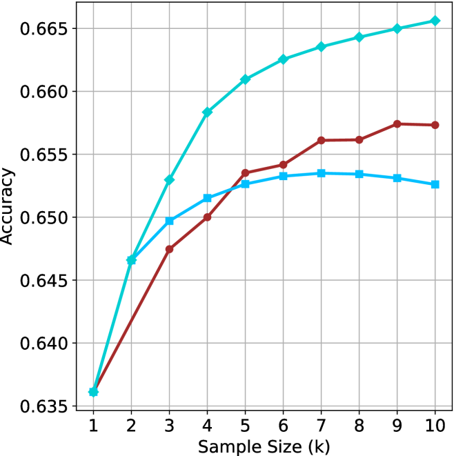
## Line Chart: Accuracy vs. Sample Size (k) ### Overview The image is a line chart plotting "Accuracy" on the vertical y-axis against "Sample Size (k)" on the horizontal x-axis. It displays the performance trends of three distinct methods or models as the sample size increases from 1 to 10 (in thousands, denoted by 'k'). All three series begin at the same accuracy point for the smallest sample size but diverge as the sample size grows. ### Components/Axes * **X-Axis (Horizontal):** * **Label:** "Sample Size (k)" * **Scale:** Linear, with major tick marks and labels at integer values from 1 to 10. * **Y-Axis (Vertical):** * **Label:** "Accuracy" * **Scale:** Linear, with major tick marks and labels at intervals of 0.005, ranging from 0.635 to 0.665. * **Data Series (Lines):** Three distinct lines are plotted, differentiated by color and marker shape. There is no explicit legend box within the chart area; identification is based on visual attributes. 1. **Cyan Line with Diamond Markers:** The top-performing series. 2. **Red (Maroon) Line with Circle Markers:** The middle-performing series. 3. **Blue Line with Square Markers:** The lowest-performing series after the initial point. * **Grid:** A light gray grid is present, with vertical lines at each x-axis tick and horizontal lines at each y-axis tick. ### Detailed Analysis **Trend Verification & Data Point Extraction (Approximate Values):** * **Cyan Line (Diamonds):** Shows a strong, consistent upward trend that begins to plateau slightly at higher sample sizes. * (k=1, ~0.636) -> (k=2, ~0.647) -> (k=3, ~0.653) -> (k=4, ~0.658) -> (k=5, ~0.661) -> (k=6, ~0.6625) -> (k=7, ~0.6635) -> (k=8, ~0.664) -> (k=9, ~0.665) -> (k=10, ~0.6655) * **Red Line (Circles):** Shows a steady upward trend that flattens significantly after k=7. * (k=1, ~0.636) -> (k=2, ~0.642) -> (k=3, ~0.6475) -> (k=4, ~0.650) -> (k=5, ~0.6535) -> (k=6, ~0.654) -> (k=7, ~0.656) -> (k=8, ~0.656) -> (k=9, ~0.6575) -> (k=10, ~0.6575) * **Blue Line (Squares):** Shows an initial upward trend that peaks around k=7 and then exhibits a slight downward trend. * (k=1, ~0.636) -> (k=2, ~0.647) -> (k=3, ~0.650) -> (k=4, ~0.6515) -> (k=5, ~0.6525) -> (k=6, ~0.653) -> (k=7, ~0.6535) -> (k=8, ~0.6535) -> (k=9, ~0.653) -> (k=10, ~0.6525) ### Key Observations 1. **Common Origin:** All three methods start at the same accuracy (~0.636) when the sample size is smallest (k=1). 2. **Divergence with Scale:** Performance diverges immediately as sample size increases. The cyan method shows the most significant and sustained improvement. 3. **Performance Hierarchy:** A clear and consistent hierarchy is established from k=2 onward: Cyan > Red > Blue. 4. **Plateauing Effects:** All three curves show signs of diminishing returns. The cyan curve's growth slows after k=6. The red curve plateaus after k=7. The blue curve peaks at k=7 and then slightly regresses. 5. **Relative Gains:** At the largest sample size (k=10), the cyan method's accuracy is approximately 0.0295 points higher than the blue method's, representing a substantial relative improvement. ### Interpretation This chart demonstrates the relationship between training/evaluation sample size and model accuracy for three different approaches. The data suggests that: * **More Data Generally Helps:** All methods benefit from increased sample size, at least initially. * **Method Scalability Differs Dramatically:** The primary insight is the stark difference in how effectively each method leverages additional data. The cyan method is highly scalable, converting larger datasets into significant accuracy gains. The red method scales moderately well but hits a performance ceiling. The blue method scales poorly, with its optimal performance achieved at a moderate sample size (k=7), after which additional data may introduce noise or lead to slight overfitting, causing a minor decline. * **Practical Implication:** For applications where large datasets are available, the cyan method is the clear choice. If computational resources or data availability are limited to moderate sizes (k around 5-7), the performance gap between the methods is smaller, though the cyan method still leads. The blue method appears unsuitable for scenarios with very large datasets. The chart provides a visual rationale for selecting a model based on expected data scale.

## Line Graph: Model Accuracy vs. Sample Size ### Overview The image depicts a line graph comparing the accuracy of three models (Model A, Model B, Model C) across varying sample sizes (k = 1 to 10). Accuracy is measured on the y-axis (0.635–0.665), while the x-axis represents sample size. All three models show increasing accuracy with larger sample sizes, but their growth rates and final performance differ. ### Components/Axes - **X-axis**: "Sample Size (k)" with integer markers from 1 to 10. - **Y-axis**: "Accuracy" with decimal markers from 0.635 to 0.665. - **Legend**: Located in the top-right corner, associating: - Teal line → "Model A" - Red line → "Model B" - Blue line → "Model C" ### Detailed Analysis 1. **Model A (Teal Line)**: - Starts at **0.635** when k=1. - Increases steadily, reaching **0.665** at k=10. - Slope is consistently upward, with no plateaus. 2. **Model B (Red Line)**: - Begins at **0.635** (k=1). - Sharp rise to **0.655** by k=3. - Plateaus between k=3 and k=10, maintaining **~0.655–0.657** accuracy. 3. **Model C (Blue Line)**: - Starts at **0.635** (k=1). - Gradual increase to **~0.652** at k=10. - Slope is less steep than Model A but steeper than Model B after k=5. ### Key Observations - **Model A** achieves the highest accuracy across all sample sizes, particularly dominant at larger k (e.g., 0.665 vs. 0.657 for Model B at k=10). - **Model B** shows rapid early improvement but stagnates after k=3, suggesting diminishing returns. - **Model C** exhibits the slowest growth but maintains consistent upward trends without plateaus. - No lines intersect, indicating no model overtakes another in performance after their initial trajectories. ### Interpretation The data suggests that **larger sample sizes improve model accuracy**, with **Model A** being the most effective overall. Model B’s early gains but subsequent plateau imply it may be optimized for smaller datasets, while Model C’s steady growth indicates robustness but lower efficiency. The absence of crossing lines confirms that performance hierarchies remain stable across sample sizes. This could inform resource allocation: prioritize Model A for large-scale tasks, Model B for small datasets, and Model C for scenarios requiring gradual improvement.