## Heatmaps and Line Graphs: Environmental Sound Analysis
### Overview
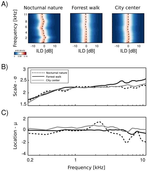
The image presents three heatmaps (A) and two line graphs (B, C) analyzing sound characteristics across three environments: "Nocturnal nature," "Forrest walk," and "City center." The heatmaps visualize frequency-intensity relationships, while the line graphs track scale (σ) and location (μ) metrics across frequencies.
### Components/Axes
**A) Heatmaps**
- **X-axis**: ILD [dB] (Intensity Level Difference), ranging from -10 to +10 dB.
- **Y-axis**: Frequency [kHz], ranging from 2 to 11 kHz.
- **Color Scale**: Probability density (0 to 0.16), with blue (low) to red (high).
- **Legend**: Bottom-left, indicating "prob density" with a gradient bar.
- **Annotations**: Dashed vertical lines in each heatmap (position varies slightly).
**B) Line Graph (Scale - σ)**
- **X-axis**: Frequency [kHz], 0.2 to 10 kHz.
- **Y-axis**: Scale - σ (unitless, 1.5 to 3).
- **Lines**:
- Dashed: Nocturnal nature (peaks at ~1 kHz, ~2.5 σ).
- Solid: Forrest walk (steady increase to ~2.8 σ at 10 kHz).
- Gray: City center (flat ~2.5 σ, minor fluctuations).
- **Legend**: Top-right, matching line styles to labels.
**C) Line Graph (Location - μ)**
- **X-axis**: Frequency [kHz], 0.2 to 10 kHz.
- **Y-axis**: Location - μ (unitless, -4 to +2).
- **Lines**:
- Dashed: Nocturnal nature (oscillates between -1 and +1 μ).
- Solid: Forrest walk (stable near 0 μ).
- Gray: City center (peaks at ~1.5 μ at 5 kHz, dips to -2 μ at 10 kHz).
- **Legend**: Top-right, consistent with B.
### Detailed Analysis
**A) Heatmaps**
- **Nocturnal nature**: Vertical orange band centered at 0 dB ILD, broadening at 4–6 kHz.
- **Forrest walk**: Narrower orange band at 0 dB ILD, sharper at 3–5 kHz.
- **City center**: Broadest orange band at 0 dB ILD, extending to ±5 dB ILD.
**B) Scale - σ Trends**
- **Nocturnal nature**: Peaks at ~1 kHz (2.5 σ), then declines.
- **Forrest walk**: Gradual rise from 1.8 σ (0.2 kHz) to 2.8 σ (10 kHz).
- **City center**: Flat ~2.5 σ, minor dip at 3 kHz.
**C) Location - μ Trends**
- **Nocturnal nature**: Sinusoidal pattern (0.2–10 kHz: -1 to +1 μ).
- **Forrest walk**: Stable near 0 μ, slight dip at 5 kHz.
- **City center**: Peaks at 1.5 μ (5 kHz), drops to -2 μ (10 kHz).
### Key Observations
1. **Heatmaps**: City center shows broader ILD spread, suggesting higher frequency variability.
2. **Line Graphs**:
- **Scale (σ)**: Forrest walk exhibits the highest σ at high frequencies.
- **Location (μ)**: City center has the most pronounced μ fluctuations.
3. **Dashed Lines**: In heatmaps, align with frequency peaks in line graphs (e.g., 1 kHz in B).
### Interpretation
The data suggests environmental differences in sound propagation:
- **Nocturnal nature** and **Forrest walk** show localized frequency-intensity peaks, likely due to natural acoustic reflections.
- **City center** exhibits broader ILD distributions and μ variability, indicating urban noise complexity (e.g., reflections, reverberation).
- **Scale (σ)** trends imply that sound energy distribution is most variable in urban settings at high frequencies.
- **Location (μ)** anomalies in the city center may reflect interference patterns from dense infrastructure.
The dashed lines in heatmaps correlate with σ peaks in line graphs, suggesting a relationship between intensity distribution and scale metrics. Urban environments demonstrate greater acoustic heterogeneity compared to natural settings.