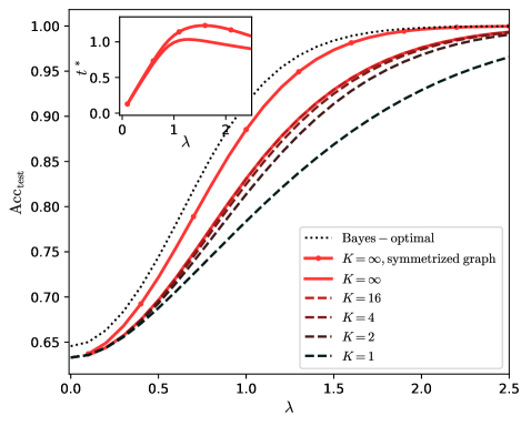
## Line Graph: Test Accuracy vs. Regularization Parameter (λ) ### Overview The graph depicts the relationship between the regularization parameter λ and test accuracy (Acc_test) for different model configurations. A secondary inset graph highlights the behavior near λ=0. The primary trend shows test accuracy increasing with λ up to a point before plateauing, with performance varying by model complexity (K). ### Components/Axes - **X-axis (λ)**: Regularization parameter ranging from 0.0 to 2.5. - **Y-axis (Acc_test)**: Test accuracy ranging from 0.65 to 1.00. - **Legend**: Located in the bottom-right corner, with six entries: - Dotted black: Bayes – optimal - Solid red: K = ∞, symmetrized graph - Dashed red: K = ∞ - Dashed brown: K = 16 - Dashed maroon: K = 4 - Dashed black: K = 2 - Solid black: K = 1 ### Detailed Analysis 1. **Bayes – optimal (dotted black line)**: - Remains consistently above all other lines across all λ values. - Peaks at λ ≈ 1.2 with Acc_test ≈ 0.99, then plateaus. - Spatial grounding: Topmost line, positioned centrally in the graph. 2. **K = ∞, symmetrized graph (solid red line)**: - Second-highest performance, closely tracking the Bayes-optimal line. - Peaks at λ ≈ 1.1 with Acc_test ≈ 0.985, then plateaus. - Spatial grounding: Directly below the Bayes-optimal line. 3. **K = ∞ (dashed red line)**: - Third-highest performance, slightly below the solid red line. - Peaks at λ ≈ 1.0 with Acc_test ≈ 0.98, then plateaus. - Spatial grounding: Below the solid red line, with dashed pattern. 4. **K = 16 (dashed brown line)**: - Peaks at λ ≈ 0.8 with Acc_test ≈ 0.95, then declines slightly. - Spatial grounding: Below K = ∞ lines, with a noticeable dip after λ=1. 5. **K = 4 (dashed maroon line)**: - Peaks at λ ≈ 0.6 with Acc_test ≈ 0.92, then declines. - Spatial grounding: Below K = 16, with a steeper decline post-λ=1. 6. **K = 2 (dashed black line)**: - Peaks at λ ≈ 0.4 with Acc_test ≈ 0.88, then declines. - Spatial grounding: Below K = 4, with a pronounced downward trend after λ=0.5. 7. **K = 1 (solid black line)**: - Lowest performance, peaks at λ ≈ 0.2 with Acc_test ≈ 0.85. - Spatial grounding: Bottommost line, with minimal improvement beyond λ=0.3. **Inset Graph**: - Zoomed-in view of the main graph’s lower-left region (λ=0 to 2, Acc_test=0.65 to 1.0). - Confirms the trend of increasing accuracy with λ up to λ=1, then plateauing. - Highlights the divergence between high-K and low-K models at small λ values. ### Key Observations 1. **Optimal λ**: All models achieve peak performance near λ=1, with Bayes-optimal and K=∞ configurations performing best. 2. **Model Complexity Trade-off**: Higher K values (e.g., K=∞) achieve higher accuracy but require larger λ to avoid overfitting. Lower K values (e.g., K=1) underperform but are less sensitive to λ. 3. **Performance Saturation**: Beyond λ=1.5, all models plateau, suggesting diminishing returns from increased regularization. 4. **Inset Confirmation**: The zoomed-in view validates the main trend, emphasizing the critical region near λ=0 where performance differences are most pronounced. ### Interpretation The graph demonstrates that model complexity (K) and regularization (λ) are interdependent factors in achieving optimal test accuracy. The Bayes-optimal configuration (dotted black line) represents the theoretical upper bound, while practical models (K=∞, K=16, etc.) approach this bound with appropriate λ tuning. The inset graph underscores that even small λ values significantly impact performance for low-K models, but higher-K models require larger λ to balance complexity and generalization. The plateau at λ>1.5 suggests that excessive regularization degrades performance, reinforcing the need for careful hyperparameter tuning. The spatial alignment of lines (e.g., K=∞ configurations clustering near the top) visually reinforces the trade-off between model capacity and regularization strength.