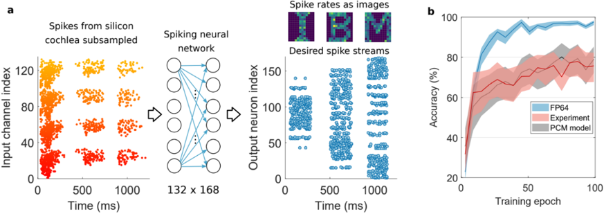
## Diagram and Chart: Spiking Neural Network Performance ### Overview The image presents a diagram of a spiking neural network processing data from a silicon cochlea, along with a chart comparing the accuracy of different models (FP64, Experiment, PCM model) during training. ### Components/Axes **Part a (Left Side):** * **Title:** Spikes from silicon cochlea subsampled * **X-axis:** Time (ms), ranging from 0 to 1000. * **Y-axis:** Input channel index, ranging from 0 to 120. * **Data:** A scatter plot showing spike events over time, with the color of the points varying from red (at lower channel indices) to yellow/orange (at higher channel indices). The spikes are clustered in four vertical bands, each containing three sub-bands. * **Title:** Spiking neural network * **Description:** A diagram of a neural network with an input layer of 6 nodes, and an output layer of 6 nodes. The dimensions of the network are labeled as "132 x 168". * **Title:** Desired spike streams * **X-axis:** Time (ms), ranging from 0 to 1000. * **Y-axis:** Output neuron index, ranging from 0 to 150. * **Data:** A scatter plot showing spike events over time. The spikes are clustered in three vertical bands. * **Title:** Spike rates as images * **Description:** Three images depicting the letters "I", "B", and "M". **Part b (Right Side):** * **Title:** Accuracy vs. Training Epoch * **X-axis:** Training epoch, ranging from 0 to 100. * **Y-axis:** Accuracy (%), ranging from 20 to 100. * **Legend:** Located in the bottom-right corner. * **FP64:** Blue line with a blue shaded region indicating variance. * **Experiment:** Red line with a red shaded region indicating variance. * **PCM model:** Gray line with a gray shaded region indicating variance. ### Detailed Analysis **Part a (Left Side):** * **Spikes from silicon cochlea subsampled:** The spike events appear to increase in frequency over time within each of the four main bands. The color gradient suggests that lower channel indices (red) are activated earlier than higher channel indices (yellow/orange). * **Spiking neural network:** The diagram shows a fully connected network. * **Desired spike streams:** The spike events are clustered into three distinct vertical bands, corresponding to the three letters "I", "B", and "M". **Part b (Right Side):** * **FP64 (Blue):** The accuracy increases rapidly from approximately 20% to nearly 95% within the first 20 training epochs, then plateaus. * **Experiment (Red):** The accuracy increases from approximately 20% to around 70% within the first 20 training epochs, then fluctuates between 70% and 80% for the remaining epochs. * **PCM model (Gray):** The accuracy increases from approximately 20% to around 80% within the first 50 training epochs, then plateaus. ### Key Observations * The FP64 model achieves the highest accuracy and converges faster than the other two models. * The Experiment and PCM models have similar performance, with the PCM model showing a slightly smoother learning curve. * The silicon cochlea data is processed by the spiking neural network to produce desired spike streams that represent the letters "I", "B", and "M". ### Interpretation The data suggests that the FP64 model is the most effective for this particular task, achieving higher accuracy with fewer training epochs. The spiking neural network is successfully processing the input from the silicon cochlea to generate spike streams that correspond to specific letters. The experiment and PCM models show comparable performance, indicating that they may be viable alternatives, although not as efficient as the FP64 model. The diagram illustrates the flow of information from the silicon cochlea, through the spiking neural network, and into the desired output spike streams.

## Diagram & Chart: Spiking Neural Network Training Accuracy ### Overview The image presents a diagram illustrating a spiking neural network setup alongside a chart showing the training accuracy of different models over training epochs. The diagram depicts the flow of spikes from a silicon cochlea through a spiking neural network to desired spike streams. The chart shows the accuracy (%) of three models (FP64, Experiment, and PCM model) as a function of training epoch. ### Components/Axes **Diagram (a):** * **Left Plot:** Scatter plot of "Spikes from silicon cochlea subsampled". X-axis: "Time (ms)", ranging from 0 to 1000. Y-axis: "Input channel index", ranging from 0 to 120. Data points are colored orange and red. * **Center Diagram:** Representation of a "Spiking neural network". It shows a network with 132 input nodes and 168 output nodes, connected by lines representing synaptic connections. * **Right Plot:** Scatter plot of "Desired spike streams". X-axis: "Time (ms)", ranging from 0 to 1000. Y-axis: "Output neuron index", ranging from 0 to 150. Data points are colored blue. * **Top-Right:** Four images representing "Spike rates as images", each a 4x4 grid of colored squares. **Chart (b):** * X-axis: "Training epoch", ranging from 0 to 100. * Y-axis: "Accuracy (%)", ranging from 20 to 100. * Three lines representing different models: * FP64 (teal) * Experiment (red) * PCM model (grey) * Shaded areas around each line represent the standard deviation or confidence interval. ### Detailed Analysis or Content Details **Diagram (a):** * The left plot shows two distinct clusters of orange and red points, suggesting two different spike patterns over time. The orange points are concentrated between 0-500ms and 80-120 input channel index, while the red points are concentrated between 500-1000ms and 0-40 input channel index. * The spiking neural network diagram shows a fully connected layer with 132 input nodes and 168 output nodes. * The right plot shows a dense pattern of blue points, indicating a consistent stream of spikes across all output neurons and time. **Chart (b):** * **FP64:** The teal line starts at approximately 50% accuracy at epoch 0 and rises sharply to around 95% accuracy by epoch 50. It plateaus around 95-98% for the remainder of the training epochs. * **Experiment:** The red line starts at approximately 45% accuracy at epoch 0 and rises steadily to around 85% accuracy by epoch 100. The shaded area around the line indicates a significant amount of variability in the accuracy. * **PCM model:** The grey line starts at approximately 40% accuracy at epoch 0 and rises steadily to around 75% accuracy by epoch 100. The shaded area around the line indicates a significant amount of variability in the accuracy. ### Key Observations * The FP64 model achieves the highest accuracy and converges quickly. * The Experiment and PCM models show slower convergence and lower overall accuracy. * The Experiment and PCM models have larger variability in accuracy compared to the FP64 model. * The spike patterns in the silicon cochlea (left plot) are distinct, suggesting different auditory stimuli. ### Interpretation The diagram illustrates a computational model of auditory processing, where spikes from a silicon cochlea are processed by a spiking neural network to generate desired spike streams. The chart shows the training accuracy of different models used to implement this network. The FP64 model, likely a high-precision floating-point model, demonstrates superior performance, suggesting that higher precision is beneficial for training this type of network. The Experiment and PCM models, potentially lower-precision or alternative implementations, show lower accuracy and greater variability, indicating challenges in achieving comparable performance with these approaches. The difference in accuracy between the models could be due to the limitations of lower-precision arithmetic or the specific architecture of the PCM model. The distinct spike patterns in the silicon cochlea suggest that the network is capable of processing different auditory stimuli. The overall results suggest that while spiking neural networks hold promise for auditory processing, careful consideration must be given to the precision and architecture of the models used to implement them.

\n ## Diagram and Chart: Spiking Neural Network Processing and Training Accuracy ### Overview The image is a two-panel technical figure (labeled **a** and **b**) illustrating a neuromorphic computing pipeline and its performance. Panel **a** is a schematic diagram showing the flow of data from a silicon cochlea through a spiking neural network to produce desired output spike streams. Panel **b** is a line chart comparing the training accuracy over epochs for three different computational models. ### Components/Axes **Panel a: Schematic Diagram** * **Left Section (Input):** A scatter plot titled "Spikes from silicon cochlea subsampled". * **Y-axis:** "Input channel index" (Range: 0 to ~130). * **X-axis:** "Time (ms)" (Range: 0 to ~1200 ms). * **Data:** Clusters of colored dots (gradient from red at low indices to yellow at high indices) representing spike events across channels over time. * **Middle Section (Processing):** A diagram of a "Spiking neural network". * Depicted as a fully connected layer of circles (neurons) with arrows (synaptic connections). * Text below: "132 x 168", likely indicating the network's weight matrix dimensions (132 input channels by 168 output neurons). * **Right Section (Output):** Two sub-plots. 1. **Top:** Three small heatmaps titled "Spike rates as images". These are 2D representations (likely spatial or spectro-temporal) of spike rate data. 2. **Bottom:** A scatter plot titled "Desired spike streams". * **Y-axis:** "Output neuron index" (Range: 0 to ~160). * **X-axis:** "Time (ms)" (Range: 0 to ~1200 ms). * **Data:** Clusters of blue dots representing the target spike patterns for the output neurons. **Panel b: Line Chart** * **Title:** None explicit, but the content is "Accuracy vs. Training epoch". * **Y-axis:** "Accuracy (%)" (Range: 20% to 100%). * **X-axis:** "Training epoch" (Range: 0 to 100). * **Legend (Bottom-right corner):** * **FP64:** Blue line with light blue shaded variance region. * **Experiment:** Red line with light red shaded variance region. * **PCM model:** Gray line with light gray shaded variance region. ### Detailed Analysis **Panel a: Data Flow** 1. **Input Spike Data:** The "Spikes from silicon cochlea subsampled" plot shows non-uniform, bursty spiking activity across ~130 input channels over a 1.2-second window. The color gradient (red to yellow) correlates with the input channel index. 2. **Network Transformation:** This spike data is fed into a spiking neural network with a 132x168 connectivity structure. 3. **Output Target:** The network's goal is to produce the "Desired spike streams," which are distinct, structured patterns of blue spikes across ~160 output neurons over the same time window. The "Spike rates as images" likely provide an alternative, condensed view of these target patterns. **Panel b: Training Performance Trends** * **FP64 (Blue Line):** Shows the highest and most stable performance. It rises steeply from ~30% accuracy at epoch 0, surpasses 80% by epoch ~10, and plateaus near 95-98% accuracy from epoch ~40 onward. The shaded variance region is relatively narrow. * **Experiment (Red Line):** Shows the lowest and most variable performance. It starts near 20%, rises to ~60% by epoch ~10, and then fluctuates between approximately 65% and 80% for the remainder of training. The shaded variance region is very wide, indicating high run-to-run variability. * **PCM model (Gray Line):** Performs between the other two. It follows a similar initial rise to the FP64 line but plateaus at a lower level, around 80-85% accuracy. Its variance region is wider than FP64's but narrower than the Experiment's. ### Key Observations 1. **Performance Hierarchy:** There is a clear and consistent hierarchy in final accuracy: FP64 (best) > PCM model > Experiment (worst). 2. **Convergence Speed:** The FP64 model converges to its high accuracy plateau fastest. The PCM model converges to a lower plateau at a similar initial rate. The Experiment model shows slower and less stable convergence. 3. **Stability/Variance:** The "Experiment" data series exhibits significantly higher variance (wider shaded area) compared to the computational models (FP64 and PCM), suggesting less reproducible results in the physical experimental setup. 4. **Diagram Flow:** Panel **a** establishes a clear cause-and-effect pipeline: biological-inspired input (silicon cochlea) -> computational core (SNN) -> desired functional output (spike streams). ### Interpretation This figure demonstrates the implementation and benchmarking of a neuromorphic system. Panel **a** details the specific task: training a spiking neural network to transform realistic, asynchronous input spike patterns (from a silicon cochlea sensor) into structured, desired output spike patterns. This is a common paradigm in sensory processing or pattern recognition for neuromorphic hardware. Panel **b** provides a critical performance comparison. The **FP64** line likely represents a software "gold standard" simulation using high-precision (64-bit floating-point) math, showing the algorithm's theoretical potential. The **PCM model** likely represents a simulation incorporating the non-ideal characteristics of Phase-Change Memory (PCM) devices used to implement the network's synapses in hardware. Its lower accuracy shows the performance cost of device-level non-idealities. The **Experiment** line represents results from the actual physical hardware chip. Its lower accuracy and high variance highlight the compounded challenges of real-world implementation, including device variability, noise, and circuit imperfections beyond those captured in the PCM model. **The key takeaway** is the quantification of the "reality gap": moving from an ideal algorithm (FP64) to a device-aware simulation (PCM model) and finally to physical hardware (Experiment) results in progressive degradation of accuracy and stability. This underscores the challenges in translating neuromorphic algorithms to efficient, reliable hardware.

## Diagram: Spiking Neural Network Processing and Training Performance ### Overview The image contains two primary components: 1. **Part a**: A spiking neural network (SNN) architecture processing subsampled cochlear spikes into desired spike streams. 2. **Part b**: A line graph comparing training accuracy across epochs for three models (FP64, Experiment, PCM). --- ### Components/Axes #### Part a - **Left Panel**: - **Y-axis**: Input channel index (0–120). - **X-axis**: Time (ms, 0–1000). - **Data**: Heatmap of spike activity (red = low rate, yellow = high rate) from a silicon cochlea subsampled. - **Center Diagram**: - **Neural Network**: 132×168 connections (input to output layer). - **Arrows**: Indicate flow from input spikes to output neuron indices. - **Right Panel**: - **Y-axis**: Output neuron index (0–150). - **X-axis**: Time (ms, 0–1000). - **Data**: Desired spike streams (blue dots) and spike rates visualized as images (labeled "IBM" three times). #### Part b - **X-axis**: Training epoch (0–100). - **Y-axis**: Accuracy (%) (20–100). - **Legend**: - **Blue**: FP64 (solid line). - **Red**: Experiment (dashed line with shaded confidence interval). - **Gray**: PCM model (dotted line with shaded confidence interval). --- ### Detailed Analysis #### Part a - **Spike Distribution**: - Spikes cluster in specific input channels (e.g., channels 0–20 show high activity in early time bins). - Subsampling reduces temporal resolution (e.g., sparse spikes in later time bins). - **Neural Network**: - 132 input neurons → 168 output neurons. - Output neuron indices range from 0 to 150, with sparse activation patterns. - **Desired Spike Streams**: - Blue dots represent target spike timings. - IBM images (likely placeholders) suggest categorical spike patterns. #### Part b - **FP64 Model**: - Starts at ~20% accuracy (epoch 0), rises sharply to ~95% by epoch 50, then plateaus. - Confidence interval narrows as training progresses. - **Experiment Model**: - Begins at ~30%, fluctuates between 50–80%, with wider confidence intervals. - Peaks at ~85% by epoch 100. - **PCM Model**: - Starts at ~20%, rises slowly to ~60%, with the widest confidence intervals. --- ### Key Observations 1. **Part a**: - The SNN maps cochlear spike patterns (input) to structured output streams, suggesting temporal coding. - IBM images may represent predefined spike templates for specific tasks. 2. **Part b**: - FP64 outperforms both Experiment and PCM models, indicating higher precision. - PCM model’s lower accuracy and wider confidence intervals suggest instability or approximation errors. --- ### Interpretation - **Neural Network Functionality**: The SNN transforms raw cochlear spike data into discrete output streams, likely for tasks like speech recognition or auditory processing. The IBM images may encode specific phonetic or rhythmic patterns. - **Training Performance**: - FP64’s dominance highlights the importance of numerical precision in training SNNs. - The Experiment model bridges FP64 and PCM, suggesting real-world implementations face trade-offs between accuracy and computational constraints. - PCM’s poor performance implies it may lack the capacity or optimization to handle complex spike dynamics. - **Critical Insights**: - Subsampling cochlear data risks losing temporal resolution, which the SNN partially compensates for via learned spike timing. - The PCM model’s wide confidence intervals indicate high variance in training, possibly due to hardware limitations or simplified architecture. - FP64’s plateau at ~95% suggests near-optimal performance for this task, leaving little room for improvement. - **Anomalies**: - The IBM images in part a are ambiguous; their repetition may indicate a placeholder or error in the diagram. - The Experiment model’s fluctuating accuracy could reflect dataset variability or overfitting.