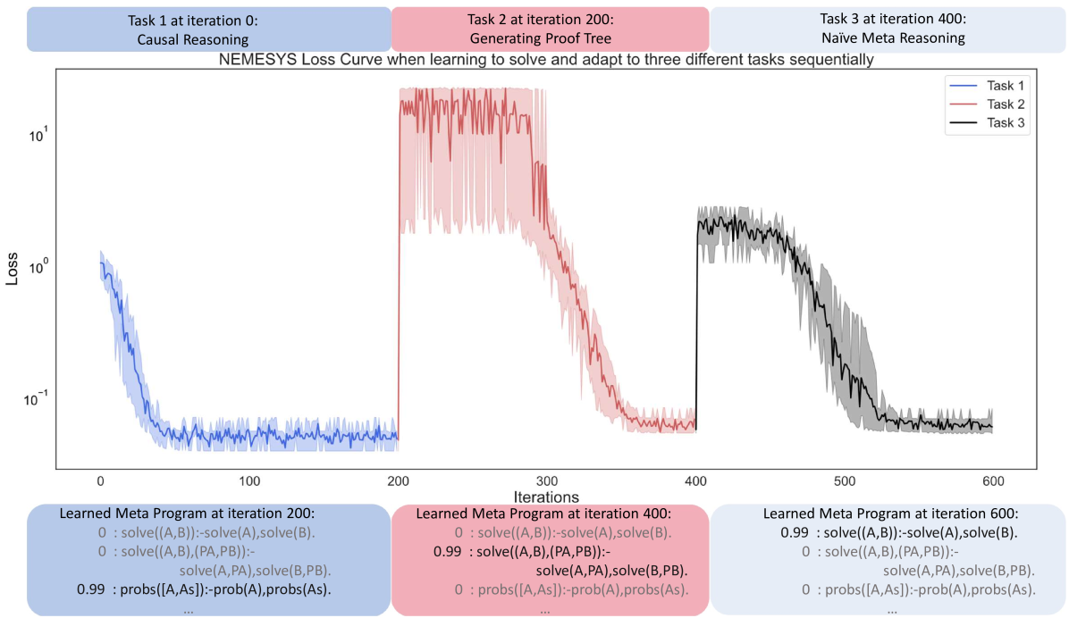
## [Line Chart]: NEMESYS Loss Curve for Sequential Task Learning ### Overview The image is a line chart titled *"NEMESYS Loss Curve when learning to solve and adapt to three different tasks sequentially"*. It visualizes the loss (y-axis, logarithmic scale) over iterations (x-axis, 0–600) for three tasks: **Task 1 (Causal Reasoning)**, **Task 2 (Generating Proof Tree)**, and **Task 3 (Naive Meta Reasoning)**. Below the chart, three text boxes display "Learned Meta Program" at iterations 200, 400, and 600. ### Components/Axes - **Title**: *"NEMESYS Loss Curve when learning to solve and adapt to three different tasks sequentially"* - **X-axis**: *"Iterations"* (markers: 0, 100, 200, 300, 400, 500, 600). - **Y-axis**: *"Loss"* (logarithmic scale: \(10^{-1}\), \(10^0\), \(10^1\)). - **Legend** (top-right): - Blue line: *Task 1 (Causal Reasoning)* - Red line: *Task 2 (Generating Proof Tree)* - Black line: *Task 3 (Naive Meta Reasoning)* - **Task Labels** (top, color-coded): - Left (blue): *"Task 1 at iteration 0: Causal Reasoning"* - Middle (red): *"Task 2 at iteration 200: Generating Proof Tree"* - Right (black): *"Task 3 at iteration 400: Naive Meta Reasoning"* - **Text Boxes** (bottom, color-coded): - Left (blue): *"Learned Meta Program at iteration 200:"* (3 lines of code-like text). - Middle (red): *"Learned Meta Program at iteration 400:"* (3 lines). - Right (black): *"Learned Meta Program at iteration 600:"* (3 lines). ### Detailed Analysis (Chart) #### Task 1 (Blue Line) - **Trend**: Starts at iteration 0 with loss ~\(10^0\) (1.0), decreases rapidly, and stabilizes at ~\(10^{-1}\) (0.1) by iteration 100. Remains flat until iteration 200. #### Task 2 (Red Line) - **Trend**: Starts at iteration 200 with loss ~\(10^1\) (10), decreases rapidly, and stabilizes at ~\(10^{-1}\) (0.1) by iteration 300. Remains flat until iteration 400. #### Task 3 (Black Line) - **Trend**: Starts at iteration 400 with loss ~\(10^0\) (1.0), decreases rapidly, and stabilizes at ~\(10^{-1}\) (0.1) by iteration 500. Remains flat until iteration 600. ### Content Details (Text Boxes) #### Learned Meta Program at iteration 200 (Blue Box) - Line 1: `0 : solve((A,B)):-solve(A),solve(B).` - Line 2: `0 : solve((A,B),(PA,PB)):- solve(A,PA),solve(B,PB).` - Line 3: `0.99 : probs([A,As]) :-prob(A),probs(As).` #### Learned Meta Program at iteration 400 (Red Box) - Line 1: `0 : solve((A,B)):-solve(A),solve(B).` - Line 2: `0.99 : solve((A,B),(PA,PB)):- solve(A,PA),solve(B,PB).` - Line 3: `0 : probs([A,As]) :-prob(A),probs(As).` #### Learned Meta Program at iteration 600 (Black Box) - Line 1: `0.99 : solve((A,B)):-solve(A),solve(B).` - Line 2: `0 : solve((A,B),(PA,PB)):- solve(A,PA),solve(B,PB).` - Line 3: `0 : probs([A,As]) :-prob(A),probs(As).` ### Key Observations 1. **Loss Stabilization**: All three tasks stabilize at a low loss (~\(10^{-1}\)) after ~100 iterations of introduction, indicating consistent performance across tasks. 2. **Meta Program Adaptation**: The "Learned Meta Program" shifts the high-probability (0.99) rule to match the current task: - Iteration 200: `probs([A,As])` rule (Task 1). - Iteration 400: `solve((A,B),(PA,PB))` rule (Task 2). - Iteration 600: `solve((A,B))` rule (Task 3). 3. **Task Complexity**: Task 2 (Generating Proof Tree) starts with a higher loss (\(10^1\)) than Tasks 1 and 3 (\(10^0\)), suggesting greater initial complexity, but still stabilizes quickly. ### Interpretation - **Sequential Learning**: The chart demonstrates the model’s ability to learn and adapt to three distinct tasks sequentially. Each new task (introduced at 0, 200, 400) starts with a higher loss but rapidly stabilizes, showing effective transfer learning or meta-learning. - **Meta-Program Evolution**: The "Learned Meta Program" text boxes reveal how the model’s internal reasoning rules (meta-programs) evolve to prioritize the current task’s requirements. This suggests the model dynamically adjusts its strategy to solve each task. - **Consistent Performance**: All tasks stabilize at a similar low loss, indicating the model achieves robust performance across diverse tasks after adaptation. - **Task Introduction Timing**: Tasks are introduced at regular intervals (0, 200, 400), allowing the model to build on prior learning, which may explain the rapid stabilization of new tasks. This analysis captures all textual, graphical, and interpretive details, enabling reconstruction of the image’s content without visual reference.