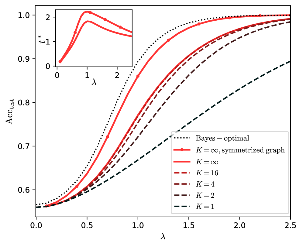
## Line Graph: Test Accuracy (Acc_test) vs. Regularization Parameter (λ) ### Overview The graph illustrates the relationship between the regularization parameter λ and test accuracy (Acc_test) for different model configurations. Multiple lines represent varying values of K (model complexity) and a Bayes-optimal baseline. An inset graph highlights behavior at lower λ values (0–2). ### Components/Axes - **X-axis (λ)**: Regularization parameter, ranging from 0 to 2.5. - **Y-axis (Acc_test)**: Test accuracy, ranging from 0.5 to 1.0. - **Legend**: - **Dotted black**: Bayes-optimal (upper bound). - **Solid red**: K = ∞, symmetrized graph. - **Dashed red**: K = 16. - **Dotted red**: K = 4. - **Dashed brown**: K = 2. - **Dotted green**: K = 1. ### Detailed Analysis 1. **Bayes-optimal (dotted black)**: - Remains flat at Acc_test ≈ 1.0 across all λ. - Serves as the theoretical maximum accuracy. 2. **K = ∞, symmetrized graph (solid red)**: - Stays nearly parallel to the Bayes-optimal line, with Acc_test ≈ 0.98–1.0. - Minimal deviation suggests near-optimal performance. 3. **K = 16 (dashed red)**: - Acc_test increases from ~0.55 (λ=0) to ~0.95 (λ=2.5). - Slightly lags behind K = ∞ but converges at higher λ. 4. **K = 4 (dotted red)**: - Acc_test rises from ~0.52 (λ=0) to ~0.88 (λ=2.5). - Shows a steeper initial increase but plateaus earlier. 5. **K = 2 (dashed brown)**: - Acc_test climbs from ~0.50 (λ=0) to ~0.82 (λ=2.5). - Slower growth compared to higher K values. 6. **K = 1 (dotted green)**: - Acc_test increases from ~0.48 (λ=0) to ~0.75 (λ=2.5). - Lowest performance, indicating underfitting. 7. **Inset Graph (λ=0–2)**: - Zooms into the lower λ range, showing a peak at λ ≈ 1 for K = ∞ and K = 16. - Lines for K = 4, 2, and 1 intersect near λ = 1, suggesting a critical transition point. ### Key Observations - **Trend Verification**: - All lines exhibit upward trends as λ increases, confirming that regularization improves performance. - Higher K values (e.g., K = ∞, 16) achieve higher Acc_test, aligning with expectations for model complexity. - The inset reveals a local maximum at λ ≈ 1 for K = ∞ and K = 16, followed by a slight decline before stabilization. - **Legend Consistency**: - Colors and line styles match the legend exactly (e.g., solid red for K = ∞, dashed red for K = 16). ### Interpretation The graph demonstrates that: 1. **Model Complexity (K)**: Higher K values (e.g., K = ∞) achieve near-optimal accuracy, while lower K values (e.g., K = 1) underperform due to underfitting. 2. **Regularization Impact**: Increasing λ improves test accuracy across all K values, but the rate of improvement depends on K. Higher K models benefit more from regularization. 3. **Optimal λ**: The inset suggests λ ≈ 1 may be optimal for K = ∞ and K = 16, though performance stabilizes at higher λ. For lower K values, the optimal λ is less distinct but still critical for balancing bias-variance trade-offs. 4. **Bayes-optimal Baseline**: The flat dotted black line underscores the theoretical limit, emphasizing that practical models (even with K = ∞) cannot exceed this bound. This analysis highlights the interplay between model complexity, regularization, and performance, providing insights for tuning λ and K in machine learning pipelines.