\n
## Line Chart: Hypothesis Function Evaluation Over Time
### Overview
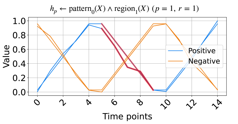
The image displays a line chart plotting two data series, labeled "Positive" and "Negative," against a sequence of time points. The chart is titled with a mathematical expression suggesting it visualizes the output of a logical hypothesis function. The two series exhibit a clear inverse relationship over the observed period.
### Components/Axes
* **Title:** Located at the top center. Text: `h_p ← pattern_0(X) ∧ region_1(X) (p = 1, r = 1)`. This is a logical expression where `∧` denotes "AND". It defines a hypothesis `h_p` as the conjunction of `pattern_0(X)` and `region_1(X)`, with parameters `p=1` and `r=1`.
* **Y-Axis:** Labeled "Value" on the left side. Scale ranges from 0.0 to 1.0, with major tick marks at 0.0, 0.2, 0.4, 0.6, 0.8, and 1.0.
* **X-Axis:** Labeled "Time points" at the bottom. Scale shows integer markers from 0 to 14, with labeled ticks at 0, 2, 4, 6, 8, 10, 12, and 14.
* **Legend:** Positioned in the center-right area of the plot. It contains two entries:
* A blue line segment labeled "Positive".
* An orange line segment labeled "Negative".
* **Data Series:**
* **Positive (Blue Line):** A smooth, continuous line.
* **Negative (Orange Line):** A smooth, continuous line.
### Detailed Analysis
**Positive Series (Blue Line) Trend & Approximate Data Points:**
The line starts near the minimum value, rises to a peak, falls to a trough, and then rises sharply again.
* Time 0: Value ≈ 0.0
* Time 4: Value ≈ 0.95 (Peak)
* Time 10: Value ≈ 0.05 (Trough)
* Time 14: Value ≈ 1.0 (Final point, highest value)
**Negative Series (Orange Line) Trend & Approximate Data Points:**
The line starts near the maximum value, falls to a trough, rises to a peak, and then falls sharply again. Its movement is the inverse of the Positive series.
* Time 0: Value ≈ 0.95
* Time 4: Value ≈ 0.05 (Trough)
* Time 10: Value ≈ 0.95 (Peak)
* Time 14: Value ≈ 0.05 (Final point)
**Relationship:** The two lines are near-perfect mirror images of each other across the horizontal midline (Value ≈ 0.5). When one is high, the other is low.
### Key Observations
1. **Inverse Correlation:** The most prominent pattern is the strong inverse relationship between the "Positive" and "Negative" values. Their peaks and troughs align at the same time points (4, 10, 14) but with opposite magnitudes.
2. **Cyclic Behavior:** Both series exhibit a cyclic pattern over the 14 time points, completing roughly one full cycle (high-to-low-to-high for Positive, low-to-high-to-low for Negative).
3. **Symmetry:** The chart is highly symmetric. The value of one series at any given time point appears to be approximately `1 - (value of the other series)`.
4. **Mathematical Context:** The title indicates this is not arbitrary data but a visualization of a specific logical function (`pattern_0 AND region_1`) being evaluated over time or across samples (`X`).
### Interpretation
This chart likely illustrates the output of a binary classifier or a logical rule applied to a dataset over time. The "Positive" and "Negative" labels probably refer to the confidence, probability, or activation level of two complementary conditions or classes.
* **What the data suggests:** The function `h_p` produces outputs where the "Positive" and "Negative" components are mutually exclusive and exhaustive. When the condition for "Positive" is strongly met (value ~1), the condition for "Negative" is not met (value ~0), and vice versa. This is characteristic of a system modeling a clear dichotomy.
* **How elements relate:** The title defines the rule, and the chart shows its dynamic application. The parameters `(p=1, r=1)` might control the sensitivity or scope of the `pattern` and `region` components of the rule.
* **Notable anomalies:** There are no apparent outliers; the data follows a very clean, smooth, and intentional pattern. This suggests the chart is likely a theoretical demonstration or the result of a controlled simulation rather than noisy empirical data.
* **Underlying meaning:** The visualization demonstrates the successful implementation of the logical conjunction (`∧`). The inverse relationship confirms that the two conditions (`pattern_0` and `region_1`) are being combined correctly to produce a single, decisive hypothesis output that flips between two states over the evaluated sequence.