\n
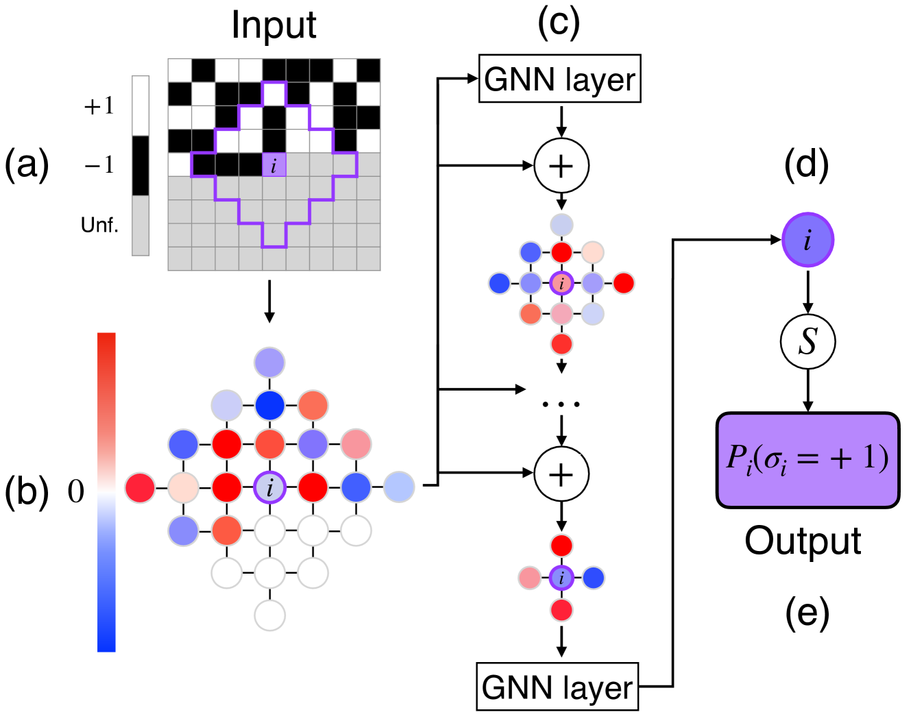
## Diagram: Graph Neural Network (GNN) Architecture for Grid-Based Probabilistic Prediction
### Overview
The image is a technical diagram illustrating a multi-stage process for using a Graph Neural Network (GNN) to predict the probability of a specific state for a target node within a grid structure. The process flows from an initial input grid, through graph construction and iterative GNN processing, to a final probabilistic output.
### Components/Axes
The diagram is segmented into five labeled components: (a), (b), (c), (d), and (e).
**Component (a): Input**
* **Title:** "Input"
* **Legend (Top-Left):**
* White square: `+1`
* Black square: `-1`
* Gray square: `Unf.` (likely abbreviation for "Unfilled" or "Unknown")
* **Content:** A 10x10 grid. The top 5 rows contain a checkerboard pattern of black (`-1`) and white (`+1`) squares. The bottom 5 rows are entirely gray (`Unf.`). A purple outline highlights a contiguous region of 13 squares (a mix of black, white, and gray) centered around a specific square labeled with the letter `i`.
**Component (b): Graph Construction**
* **Color Bar (Left):** A vertical gradient bar. The top is red, the middle is white labeled `0`, and the bottom is blue. This serves as a legend for node colors in the adjacent graph.
* **Content:** A graph representation derived from the input grid. Nodes are arranged in a lattice structure corresponding to the grid cells. Each node is colored according to the color bar (red, white, blue, or intermediate shades). The central node, corresponding to the `i` from the input, is white with a purple outline and labeled `i`. Nodes are connected by edges to their immediate neighbors.
**Component (c): GNN Processing Pipeline**
* **Content:** A vertical flowchart showing iterative processing.
1. An arrow from the graph in (b) points to a box labeled "GNN layer".
2. The output of the GNN layer goes to a circle containing a plus sign (`+`), indicating an aggregation or addition operation.
3. This produces a new graph representation (a smaller cluster of colored nodes, again with a central `i` node).
4. This process repeats, indicated by vertical ellipsis (`...`), leading to another `+` operation and a final, more refined graph representation.
5. The final graph output points to a second "GNN layer" box at the bottom.
**Component (d): Output Generation**
* **Content:** A flowchart showing the final prediction step.
1. An arrow from the final "GNN layer" in (c) points to a purple circle labeled `i`.
2. An arrow from this `i` node points down to a circle labeled `S`.
3. An arrow from `S` points to a purple rectangular box containing the mathematical expression: `P_i(σ_i = +1)`.
4. Below this box is the label "Output".
**Component (e): Label**
* **Content:** The letter `(e)` is placed in the bottom-right corner, likely serving as a figure or sub-figure label for the entire diagram.
### Detailed Analysis
1. **Input State (a):** The input is a partially observed grid. The top half has known binary states (`+1`/`-1`), while the bottom half is unknown (`Unf.`). The purple outline defines a local neighborhood or "receptive field" around the target cell `i` that is used for analysis.
2. **Graph Representation (b):** The grid is transformed into a graph where each cell is a node. The color of each node (red to blue via white) likely represents an initial feature value, possibly derived from the input state (`+1`, `-1`, `Unf.`) or an initial embedding. The central node `i` is the focus of the prediction.
3. **GNN Pipeline (c):** The graph is processed through multiple GNN layers. Each layer updates the node features by aggregating information from neighboring nodes (represented by the `+` operations). The sequence shows the node features evolving through at least two aggregation steps, resulting in progressively more refined representations of the local graph structure around node `i`.
4. **Final Prediction (d):** The final, updated feature vector for node `i` is passed through a function or module labeled `S` (which could stand for a softmax, sigmoid, or another scoring function). This produces the final output: the probability `P_i` that the state `σ_i` of node `i` is `+1`.
### Key Observations
* The diagram clearly depicts a **message-passing neural network** architecture applied to a spatial, grid-structured problem.
* The process is **local and targeted**: it focuses on predicting the state of a single node (`i`) based on its local graph neighborhood defined in the input.
* The **color coding is consistent**: the purple outline and label `i` track the target node through all stages (input grid, initial graph, intermediate GNN outputs, final prediction node).
* The **output is probabilistic**, not a deterministic classification, as indicated by the `P_i(...)` notation.
### Interpretation
This diagram illustrates a method for solving a **structured prediction problem**, likely related to statistical physics (e.g., the Ising model, given the `+1`/`-1` spins) or image inpainting (filling in the `Unf.` region). The core idea is to leverage the relational inductive bias of GNNs to make predictions about unknown parts of a system based on known parts.
The flow demonstrates how a GNN can:
1. **Encode** local grid information into a graph.
2. **Process** it through layers that propagate and transform information across the graph's connections.
3. **Decode** the final state of a specific node into a calibrated probability.
The presence of the `S` function before the final probability suggests the model outputs logits or scores that are then normalized. The entire pipeline is a self-contained model for inferring hidden states in a partially observed binary grid system.