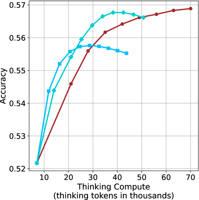
## Line Chart: Accuracy vs. Thinking Compute ### Overview The image is a line chart comparing the accuracy of different models against the "Thinking Compute" (measured in thousands of thinking tokens). Three different models are represented by three lines: a light blue line with diamond markers, a dark red line with circle markers, and a medium blue line with square markers. The chart shows how accuracy changes as the thinking compute increases. ### Components/Axes * **X-axis:** "Thinking Compute (thinking tokens in thousands)". The axis ranges from approximately 5 to 70, with tick marks at intervals of 10 (10, 20, 30, 40, 50, 60, 70). * **Y-axis:** "Accuracy". The axis ranges from 0.52 to 0.57, with tick marks at intervals of 0.01 (0.52, 0.53, 0.54, 0.55, 0.56, 0.57). * **Data Series:** * Light Blue line with diamond markers. * Dark Red line with circle markers. * Medium Blue line with square markers. * **Grid:** The chart has a grid for easier reading of values. ### Detailed Analysis * **Light Blue (Diamond Markers):** * Trend: Initially increases rapidly, peaks around x=40, then decreases slightly. * Data Points: * (8, 0.522) * (15, 0.544) * (20, 0.550) * (30, 0.560) * (40, 0.568) * (50, 0.567) * **Dark Red (Circle Markers):** * Trend: Increases steadily, then plateaus. * Data Points: * (8, 0.522) * (20, 0.547) * (30, 0.557) * (40, 0.564) * (50, 0.566) * (60, 0.568) * (70, 0.569) * **Medium Blue (Square Markers):** * Trend: Increases, peaks around x=35, then decreases. * Data Points: * (8, 0.522) * (15, 0.544) * (20, 0.550) * (30, 0.557) * (40, 0.553) * (50, 0.552) ### Key Observations * All three models start with similar accuracy at low thinking compute values. * The light blue model (diamond markers) achieves the highest accuracy initially, but its performance plateaus and then slightly decreases after a certain point. * The dark red model (circle markers) shows a consistent increase in accuracy with increasing thinking compute, eventually surpassing the other models. * The medium blue model (square markers) peaks and then declines. ### Interpretation The chart suggests that increasing "Thinking Compute" generally improves model accuracy, but the optimal amount of compute varies depending on the model architecture. The light blue model benefits less from increased compute beyond a certain point, while the dark red model continues to improve even at higher compute levels. The medium blue model's performance degrades after a certain compute level, suggesting potential overfitting or other issues. The data indicates that there is a trade-off between compute cost and accuracy, and the best model choice depends on the specific application and resource constraints.

## Line Chart: Accuracy vs. Thinking Compute ### Overview This image presents a line chart illustrating the relationship between "Thinking Compute" (measured in thousands of tokens) and "Accuracy". Three distinct data series are plotted, each represented by a different colored line. The chart appears to demonstrate how accuracy improves with increased computational effort (thinking tokens). ### Components/Axes * **X-axis:** "Thinking Compute (thinking tokens in thousands)". Scale ranges from approximately 8 to 70, with markers at 10, 20, 30, 40, 50, 60, and 70. * **Y-axis:** "Accuracy". Scale ranges from approximately 0.52 to 0.57, with markers at 0.52, 0.53, 0.54, 0.55, 0.56, and 0.57. * **Data Series:** Three lines are present, each representing a different model or configuration. * **Red Line:** Represents a data series with a generally upward trend. * **Cyan Line:** Represents a data series that initially rises sharply, plateaus, and then slightly declines. * **Blue Line:** Represents a data series that rises quickly and then plateaus. * **Grid:** A light gray grid is overlaid on the chart to aid in reading values. ### Detailed Analysis Let's analyze each line individually: * **Red Line:** This line exhibits a consistent upward trend. * At x = 10, y ≈ 0.525 * At x = 20, y ≈ 0.545 * At x = 30, y ≈ 0.56 * At x = 40, y ≈ 0.565 * At x = 50, y ≈ 0.567 * At x = 60, y ≈ 0.568 * At x = 70, y ≈ 0.57 * **Cyan Line:** This line shows a rapid initial increase, followed by a plateau and a slight decrease. * At x = 10, y ≈ 0.527 * At x = 20, y ≈ 0.55 * At x = 30, y ≈ 0.567 * At x = 40, y ≈ 0.565 * At x = 50, y ≈ 0.564 * At x = 60, y ≈ 0.562 * At x = 70, y ≈ 0.56 * **Blue Line:** This line demonstrates a quick rise and then levels off. * At x = 10, y ≈ 0.528 * At x = 20, y ≈ 0.548 * At x = 30, y ≈ 0.562 * At x = 40, y ≈ 0.562 * At x = 50, y ≈ 0.563 * At x = 60, y ≈ 0.563 * At x = 70, y ≈ 0.563 ### Key Observations * All three lines show an increase in accuracy as "Thinking Compute" increases. * The red line consistently demonstrates the highest accuracy across the entire range of "Thinking Compute". * The cyan line exhibits the most pronounced plateau and slight decline at higher "Thinking Compute" values. * The blue line reaches a plateau earlier than the red line. * The initial gains in accuracy are most significant for all three lines. ### Interpretation The chart suggests that increasing the amount of "Thinking Compute" generally leads to improved accuracy. However, there appear to be diminishing returns. The red line indicates that a particular model or configuration benefits most from increased computation, achieving the highest accuracy. The cyan line suggests that beyond a certain point, additional computation may not yield significant improvements and could even lead to a slight decrease in accuracy, potentially due to overfitting or other factors. The blue line shows a rapid initial improvement, but then plateaus, indicating that it reaches its maximum potential accuracy relatively quickly. This data could be used to optimize the allocation of computational resources. For example, it might be more efficient to invest in improving the model represented by the cyan line rather than continuing to increase the "Thinking Compute" for that model beyond a certain threshold. The chart highlights the importance of finding the right balance between computational cost and accuracy. The fact that all lines increase suggests that "Thinking Compute" is a valuable factor in improving accuracy, but the specific benefits vary depending on the model or configuration.

## Line Chart: Accuracy vs. Thinking Compute ### Overview The image is a line chart plotting model accuracy against the amount of "thinking compute" allocated, measured in thousands of thinking tokens. It displays three distinct data series, each represented by a different colored line with unique markers, showing how performance scales with increased computational resources for different approaches or models. ### Components/Axes * **X-Axis (Horizontal):** * **Label:** "Thinking Compute (thinking tokens in thousands)" * **Scale:** Linear scale from 10 to 70, with major gridlines and labels at intervals of 10 (10, 20, 30, 40, 50, 60, 70). * **Y-Axis (Vertical):** * **Label:** "Accuracy" * **Scale:** Linear scale from 0.52 to 0.57, with major gridlines and labels at intervals of 0.01 (0.52, 0.53, 0.54, 0.55, 0.56, 0.57). * **Data Series (Lines):** * **Series 1 (Cyan Line with Diamond Markers):** This line starts at the lowest compute point and shows the steepest initial improvement. * **Series 2 (Blue Line with Square Markers):** This line also starts low and rises quickly but plateaus earlier than the others. * **Series 3 (Red/Brown Line with Circle Markers):** This line starts at a similar low point but follows a steadier, more gradual upward trajectory. * **Legend:** There is no explicit legend box within the chart area. The series are differentiated solely by line color and marker shape. ### Detailed Analysis **Data Series 1: Cyan Line (Diamond Markers)** * **Trend:** Shows a rapid, near-linear increase in accuracy from low compute, peaks, and then exhibits a slight decline at the highest compute levels shown for this series. * **Approximate Data Points:** * (7k tokens, ~0.522 accuracy) * (12k tokens, ~0.544) * (18k tokens, ~0.554) * (25k tokens, ~0.560) * (30k tokens, ~0.564) * (35k tokens, ~0.567) * (40k tokens, ~0.568) **[Peak]** * (45k tokens, ~0.567) * (50k tokens, ~0.566) **Data Series 2: Blue Line (Square Markers)** * **Trend:** Rises very steeply at the lowest compute levels, then flattens into a plateau, showing minimal gains and even a slight decrease as compute increases further. * **Approximate Data Points:** * (7k tokens, ~0.522 accuracy) * (12k tokens, ~0.544) * (16k tokens, ~0.552) * (20k tokens, ~0.556) * (25k tokens, ~0.557) * (30k tokens, ~0.558) **[Plateau Start]** * (35k tokens, ~0.557) * (40k tokens, ~0.556) * (45k tokens, ~0.555) **Data Series 3: Red/Brown Line (Circle Markers)** * **Trend:** Demonstrates a consistent, monotonic increase in accuracy across the entire range of compute. Its growth is less steep initially but sustains longer, eventually surpassing the other two series. * **Approximate Data Points:** * (7k tokens, ~0.522 accuracy) * (20k tokens, ~0.546) * (28k tokens, ~0.556) * (35k tokens, ~0.561) * (42k tokens, ~0.564) * (50k tokens, ~0.566) * (58k tokens, ~0.567) * (65k tokens, ~0.568) * (70k tokens, ~0.569) **[Highest Point on Chart]** ### Key Observations 1. **Convergence at Low Compute:** All three methods start at nearly the same accuracy (~0.522) when given minimal compute (~7k tokens). 2. **Diverging Scaling Laws:** The methods scale very differently. The cyan and blue methods show strong early returns but hit diminishing returns (blue) or a peak followed by slight degradation (cyan). The red method shows a more sustainable scaling law. 3. **Crossover Point:** The red line, which initially lags behind the cyan line, crosses above it at approximately 50k thinking tokens and continues to rise, becoming the highest-performing method at the highest compute levels shown (70k tokens). 4. **Performance Ceiling:** The cyan line suggests a potential performance ceiling or even a slight negative return beyond ~40k tokens for that specific method. The blue line hits a clear ceiling earlier, around 30k tokens. ### Interpretation This chart illustrates a fundamental trade-off in AI model scaling: the relationship between computational investment (thinking tokens) and performance (accuracy). The data suggests that different model architectures, training methods, or prompting strategies (represented by the three lines) have vastly different **compute-optimal** profiles. * The **blue method** is highly efficient for low-compute scenarios but cannot leverage additional resources effectively. It would be the best choice under strict compute budgets. * The **cyan method** offers the best peak performance for a mid-range compute budget (30k-45k tokens) but may be unstable or over-optimize at higher levels, leading to performance regression. * The **red method** demonstrates the most robust and scalable behavior. While less efficient at the very low end, it continues to improve predictably with more compute, making it the superior choice if high accuracy is the primary goal and computational resources are not a limiting factor. The chart provides a visual argument for investigating why certain approaches plateau while others scale. It implies that simply adding more compute is not a universal solution; the underlying method must be capable of utilizing that compute productively. The crossover point is particularly important for decision-making, indicating the threshold at which investing in the more scalable (red) method becomes advantageous.

## Line Graph: Accuracy vs. Thinking Compute (Tokens in Thousands) ### Overview The graph compares the accuracy of three computational models (Large, Medium, Small) across varying levels of "Thinking Compute" (measured in thousands of thinking tokens). All models start at similar accuracy levels but diverge in performance as compute increases. ### Components/Axes - **X-axis**: "Thinking Compute (thinking tokens in thousands)" - Scale: 10 to 70 (increments of 10) - Labels: Numerical ticks at 10, 20, 30, 40, 50, 60, 70 - **Y-axis**: "Accuracy" - Scale: 0.52 to 0.57 (increments of 0.01) - Labels: Numerical ticks at 0.52, 0.53, 0.54, 0.55, 0.56, 0.57 - **Legend**: Top-right corner - Colors: - Red: "Large Model" - Green: "Medium Model" - Blue: "Small Model" ### Detailed Analysis 1. **Large Model (Red Line)** - **Trend**: Steady upward slope from (10, 0.52) to (70, 0.57). - **Key Points**: - At 10k tokens: 0.52 accuracy - At 30k tokens: ~0.56 accuracy - At 70k tokens: 0.57 accuracy 2. **Medium Model (Green Line)** - **Trend**: Rapid initial increase, then plateau. - **Key Points**: - At 10k tokens: 0.52 accuracy - At 30k tokens: ~0.56 accuracy - At 50k tokens: ~0.565 accuracy (plateau) 3. **Small Model (Blue Line)** - **Trend**: Sharp rise, then decline, followed by stabilization. - **Key Points**: - At 10k tokens: 0.52 accuracy - At 20k tokens: ~0.55 accuracy - At 40k tokens: ~0.545 accuracy (dip) - At 50k tokens: ~0.54 accuracy (stabilizes) ### Key Observations - **Large Model Dominance**: The red line consistently outperforms others, showing linear improvement with compute. - **Medium Model Efficiency**: The green line achieves near-peak accuracy (0.565) by 50k tokens but plateaus. - **Small Model Limitations**: The blue line peaks early (20k tokens) but degrades with additional compute, suggesting diminishing returns or overfitting. - **Convergence at Low Compute**: All models start at 0.52 accuracy at 10k tokens, indicating baseline performance parity. ### Interpretation The data suggests that **larger models scale more effectively with increased compute**, maintaining higher accuracy across all token ranges. Medium models achieve strong performance but face diminishing returns beyond 30k tokens. Small models, while initially competitive, degrade with added compute, possibly due to architectural constraints or overfitting. This highlights a trade-off between model size, compute efficiency, and accuracy in computational tasks. **Note**: All values are approximate, with uncertainty due to visual estimation from the graph.