\n
## Diagram: Cyclic Boundary Condition Illustration
### Overview
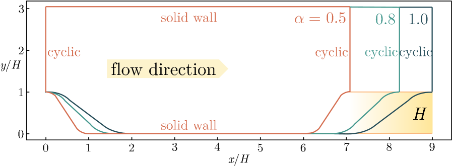
The image is a diagram illustrating cyclic boundary conditions in a flow field, likely related to computational fluid dynamics or a similar simulation. It depicts the y/H versus x/H relationship for different boundary conditions (solid wall, cyclic, and varying alpha values). The diagram shows how the flow profile changes as it encounters different boundary types.
### Components/Axes
* **x-axis:** Labeled "x/H". The scale ranges from approximately 0 to 9, with markings at integer values.
* **y-axis:** Labeled "y/H". The scale ranges from approximately 0 to 3, with markings at integer values.
* **Curves:** Three distinct curves are present, each representing a different boundary condition.
* Dark Green: Represents a "solid wall" boundary condition.
* Light Brown: Represents a "solid wall" boundary condition.
* Teal/Cyan: Represents cyclic boundary conditions with varying alpha (α) values: 0.5, 0.8, and 1.0.
* **Annotations:**
* "flow direction" - A yellow rectangular box pointing to the right, indicating the direction of the flow.
* "solid wall" - Labels above and below the dark green and light brown curves.
* "cyclic" - Labels above the teal/cyan curves.
* "α = 0.5", "α = 0.8", "α = 1.0" - Labels indicating the alpha values for the cyclic boundary conditions.
* "H" - Label indicating a reference height.
* "cycliccycliccyclic" - Repeated label above the rightmost teal/cyan curves.
### Detailed Analysis or Content Details
The diagram shows the profiles of y/H as a function of x/H for different boundary conditions.
* **Solid Wall (Dark Green):** Starts at y/H ≈ 3, decreases rapidly to y/H ≈ 0 around x/H ≈ 1, and remains at y/H ≈ 0 until x/H ≈ 3.
* **Solid Wall (Light Brown):** Starts at y/H ≈ 1, decreases rapidly to y/H ≈ 0 around x/H ≈ 7, and remains at y/H ≈ 0 until x/H ≈ 9.
* **Cyclic (α = 0.5):** Starts at y/H ≈ 2.5, decreases to y/H ≈ 0 around x/H ≈ 6, and then increases again.
* **Cyclic (α = 0.8):** Starts at y/H ≈ 2.5, decreases to y/H ≈ 0 around x/H ≈ 7, and then increases again.
* **Cyclic (α = 1.0):** Starts at y/H ≈ 2.5, decreases to y/H ≈ 0 around x/H ≈ 8, and then increases again.
The cyclic boundary conditions show a phase shift as alpha increases. The curves are vertically shifted, indicating a change in the overall flow profile. The "H" label appears to indicate a reference height, possibly the height of the domain.
### Key Observations
* The solid wall boundary conditions result in a sharp drop to y/H = 0, representing a no-flow condition at the wall.
* The cyclic boundary conditions maintain continuity of the flow across the boundary, resulting in a periodic profile.
* Increasing the alpha value (α) for the cyclic boundary condition shifts the curve to the right, indicating a change in the phase of the flow.
* The repeated "cycliccycliccyclic" label suggests the cyclic nature of the boundary condition is being emphasized.
### Interpretation
This diagram illustrates the implementation of cyclic boundary conditions in a flow simulation. Cyclic boundary conditions are used when the flow is expected to repeat itself across a certain domain boundary. The alpha (α) parameter likely controls the phase shift or offset between the repeating sections of the flow. The diagram demonstrates how different alpha values affect the flow profile near the cyclic boundary. The solid wall boundary conditions serve as a contrast, showing a completely different flow behavior where the flow is stopped at the wall. The diagram is a visual aid for understanding how to apply and interpret cyclic boundary conditions in computational fluid dynamics or related fields. The diagram does not provide numerical data, but rather a qualitative illustration of the boundary conditions.