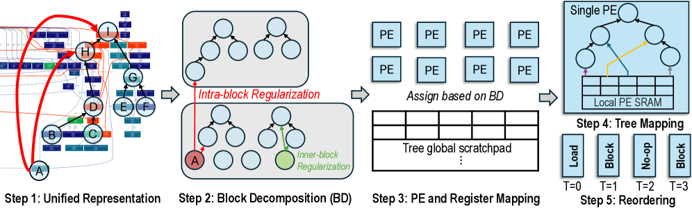
## Diagram: Computation Graph Mapping and Scheduling Process ### Overview This image illustrates a five-step technical workflow for mapping a complex computation graph (likely a neural network or decision tree) onto a hardware architecture consisting of Processing Elements (PEs). The process flows from left to right, transforming a unified graph representation into a scheduled sequence of operations on specific hardware components. ### Components/Axes The diagram is organized into five sequential steps, labeled at the bottom: 1. **Step 1: Unified Representation** (Far Left) 2. **Step 2: Block Decomposition (BD)** (Center-Left) 3. **Step 3: PE and Register Mapping** (Center) 4. **Step 4: Tree Mapping** (Top-Right) 5. **Step 5: Reordering** (Bottom-Right) ### Detailed Analysis #### Step 1: Unified Representation * **Visual:** A complex, hierarchical graph structure containing nodes labeled A through I. * **Details:** The graph is interconnected with various lines representing data flow or dependencies. * **Annotations:** Two prominent, thick red curved arrows originate from the bottom node (A) and point upward to nodes H and I, indicating long-range dependencies or specific data paths within the graph. #### Step 2: Block Decomposition (BD) * **Visual:** Two gray-shaded rectangular regions, each containing two tree-like structures. * **Annotations:** * **"Intra-block Regularization"**: A red arrow points from the bottom gray box to the top gray box, indicating a transformation or constraint applied between blocks. * **"Inner-block Regularization"**: A green arrow points to a specific green-shaded node within the bottom gray box, indicating a transformation or constraint applied within a block. * **Node A**: The bottom-left node is highlighted in red, corresponding to the starting point in Step 1. #### Step 3: PE and Register Mapping * **Visual:** * **Top:** A grid of eight blue squares, each labeled "PE" (Processing Element). * **Bottom:** A grid labeled "Tree global scratchpad". * **Text:** "Assign based on BD" is written between the PE grid and the scratchpad, indicating that the decomposition performed in Step 2 dictates how resources are allocated. #### Step 4: Tree Mapping * **Visual:** A "Single PE" block containing a tree structure. * **Components:** * The tree nodes are connected to a "Local PE SRAM" (Static Random Access Memory) at the bottom. * **Arrows:** Colored arrows (purple, yellow, gray) indicate data movement between the "Local PE SRAM" and specific nodes within the tree. #### Step 5: Reordering * **Visual:** Four vertical bars representing a timeline of operations. * **Labels:** * **T=0**: "Load" * **T=1**: "Block" * **T=2**: "No-op" (No operation) * **T=3**: "Block" ### Key Observations * **Abstraction Flow:** The diagram demonstrates a clear progression from high-level algorithmic representation (Step 1) to low-level hardware scheduling (Step 5). * **Regularization:** The use of "Intra-block" and "Inner-block" regularization suggests that the process involves optimizing the graph structure to fit hardware constraints (likely memory or compute limitations). * **Resource Allocation:** Step 3 explicitly links the logical decomposition (BD) to physical hardware resources (PEs and Scratchpad). * **Temporal Scheduling:** Step 5 introduces a temporal dimension (T=0 to T=3), showing that the mapping process concludes with a specific execution schedule, including idle cycles ("No-op"). ### Interpretation This diagram represents a **compiler or hardware-mapping pipeline** for specialized hardware accelerators (such as those used for AI inference or decision tree evaluation). 1. **Graph Partitioning:** The process begins by taking a large, unified computation graph and breaking it down into smaller, manageable "blocks" (Step 2). The "Regularization" labels suggest that this partitioning is not arbitrary; it is constrained to ensure the blocks fit within the hardware's memory or compute capabilities. 2. **Hardware Mapping:** Once partitioned, the system maps these logical blocks onto physical hardware (PEs and Scratchpad). The "Assign based on BD" text confirms that the hardware configuration is derived directly from the decomposition strategy. 3. **Execution Scheduling:** The final step (Reordering) demonstrates that the mapping is not just spatial (where data goes) but also temporal (when operations occur). The inclusion of a "No-op" cycle at T=2 suggests that the scheduler must account for hardware latency or synchronization requirements, resulting in a precise execution timeline. In essence, this is a visual representation of how a software-defined computation graph is "compiled" into a hardware-executable instruction stream.