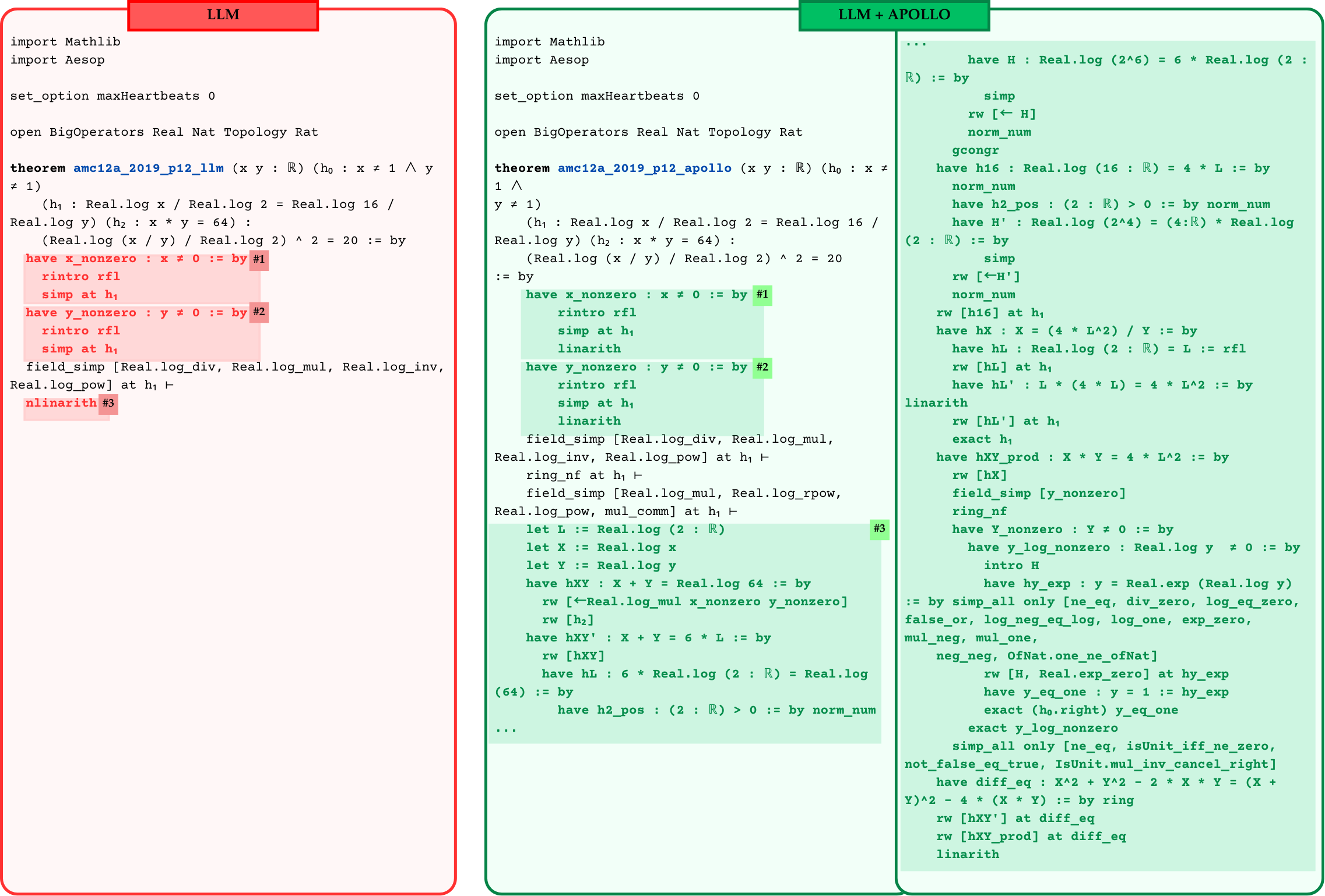
## Code Comparison: LLM vs. LLM + APOLLO ### Overview The image presents a side-by-side comparison of code snippets, labeled "LLM" (left) and "LLM + APOLLO" (right), likely representing different approaches or versions of a mathematical proof or computation. The code appears to be written in a language related to theorem proving or formal verification, possibly Lean. The comparison highlights differences in the code structure and specific commands used. ### Components/Axes * **Headers:** * Left: "LLM" (red background) * Right: "LLM + APOLLO" (green background) * **Code Blocks:** Two distinct code blocks, one under each header. * **Annotations:** Numerical annotations (#1, #2, #3) highlight specific lines or sections in each code block. * The code includes imports, options settings, theorem definitions, and proof steps. ### Detailed Analysis or ### Content Details **Left Code Block (LLM):** ```lean import Mathlib import Aesop set_option maxHeartbeats 0 open BigOperators Real Nat Topology Rat theorem amc12a_2019_p12_1lm (x y : R) (h₀ : x ≠ 1 ∧ y ≠ 1) (h₁ : Real.log x / Real.log 2 = Real.log 16 / Real.log y) (h₂ : x * y = 64) : (Real.log (x / y) / Real.log 2) ^ 2 = 20 := by have x_nonzero : x ≠ 0 := by #1 rintro rfl simp at h₁ have y_nonzero : y ≠ 0 := by #2 rintro rfl simp at h₁ field_simp [Real.log_div, Real.log_mul, Real.log_inv, Real.log_pow] at h₁ nlinarith #3 ``` **Right Code Block (LLM + APOLLO):** ```lean import Mathlib import Aesop set_option maxHeartbeats 0 open BigOperators Real Nat Topology Rat theorem amc12a_2019_p12_apollo (x y : R) (h₀ : x ≠ 1 ∧ y ≠ 1) (h₁ : Real.log x / Real.log 2 = Real.log 16 / Real.log y) (h₂ : x * y = 64) : (Real.log (x / y) / Real.log 2) ^ 2 = 20 := by have x_nonzero : x ≠ 0 := by #1 rintro rfl simp at h₁ linarith have y_nonzero : y ≠ 0 := by #2 rintro rfl simp at h₁ linarith field_simp [Real.log_div, Real.log_mul, Real.log_inv, Real.log_pow] at h₁ ring_nf at h₁ field_simp [Real.log_mul, Real.log_rpow, Real.log_pow, mul_comm] at h₁ let L := Real.log (2 : R) let X := Real.log x let Y := Real.log y have hXY : X + Y = Real.log 64 := by rw [Real.log_mul x_nonzero y_nonzero] rw [h₂] have hXY' : X + Y = 6 * L := by rw [hXY] have hL : 6 * Real.log (2 : R) = Real.log (64) := by have h₂_pos : (2 : R) > 0 := by norm_num have H : Real.log (2^6) = 6 * Real.log (2 : R) := by simp rw [← H] norm_num gcongr have h16 : Real.log (16 : R) = 4 * L := by norm_num have h₂_pos : (2 : R) > 0 := by norm_num have H' : Real.log (2^4) = (4 : R) * Real.log (2 : R) := by simp rw [← H'] norm_num rw [h16] at h₁ have hX : X = (4 * L^2) / Y := by have hL : Real.log (2 : R) = L := rfl rw [hL] at h₁ have hL' : L * (4 * L) = 4 * L^2 := by linarith rw [hL'] at h₁ exact h₁ have hXY_prod : X * Y = 4 * L^2 := by rw [hX] field_simp [y_nonzero] ring_nf have Y_nonzero : Y ≠ 0 := by have y_log_nonzero : Real.log y ≠ 0 := by intro H have hy_exp : y = Real.exp (Real.log y) := by simp_all only [ne_eq, div_zero, log_eq_zero, false_or, log_neg_eq_log, log_one, exp_zero, mul_neg, mul_one, neg_neg, OfNat.one_ne_ofNat] rw [H, Real.exp_zero] at hy_exp have y_eq_one : y = 1 := hy_exp exact (h₀.right) y_eq_one exact y_log_nonzero simp_all only [ne_eq, isUnit_iff_ne_zero, not_false_eq_true, IsUnit.mul_inv_cancel_right] have diff_eq : X^2 + Y^2 - 2 * X * Y = (X + Y)^2 - 4 * (X * Y) := by ring rw [hXY'] at diff_eq rw [hXY_prod] at diff_eq linarith ``` **Annotations:** * `#1`: Marks the "have x_nonzero" line in both code blocks. * `#2`: Marks the "have y_nonzero" line in both code blocks. * `#3`: Marks the "nlinarith" line in the LLM code block and a section of code starting with `let L := Real.log (2 : R)` in the LLM + APOLLO code block. ### Key Observations * The "LLM + APOLLO" code block is significantly longer and more detailed than the "LLM" code block. * The "LLM" code uses `nlinarith` to complete the proof, while "LLM + APOLLO" expands the proof with more explicit steps. * The "LLM + APOLLO" code introduces intermediate variables (L, X, Y) and uses rewrite rules (`rw`) extensively. * The annotations highlight key differences in the proof strategies. ### Interpretation The image illustrates the difference between a more concise proof ("LLM") and a more detailed, step-by-step proof ("LLM + APOLLO"). The "LLM + APOLLO" version likely benefits from the assistance of the APOLLO tool, which seems to guide the proof process by suggesting intermediate steps and rewrite rules. The increased verbosity in "LLM + APOLLO" may make the proof easier to understand and verify, but it comes at the cost of increased code length. The use of `linarith` in "LLM + APOLLO" suggests a more targeted approach to linear arithmetic simplification compared to the more general `nlinarith` used in "LLM". The APOLLO version breaks down the proof into smaller, more manageable steps, potentially making it more robust and easier to debug.

## Diagram: Code Comparison - LLM vs LLM + APOLLO ### Overview The image displays a side-by-side comparison of two Lean 4 code snippets attempting to formally prove a mathematical theorem (`amc12a_2019_p12`). The left panel, outlined in red and labeled "LLM", shows a short, incomplete, or failing proof attempt with specific sections highlighted in red. The right panel, outlined in green and labeled "LLM + APOLLO", shows a highly detailed, successful proof spanning two columns, with corresponding sections highlighted in green. Numbered tags (`#1`, `#2`, `#3`) are used to map specific logical steps between the two approaches, demonstrating how the "APOLLO" system corrects and expands upon the baseline LLM's output. ### Components and Layout * **Left Panel (Red Outline):** * **Header:** A red box containing the text "LLM". * **Content:** A single column of Lean 4 code. * **Highlights:** Light red background applied to lines 11-16 and line 19. * **Tags:** `#1`, `#2`, `#3` placed inline with the code. * **Right Panel (Green Outline):** * **Header:** A green box containing the text "LLM + APOLLO". * **Content:** Lean 4 code split into two columns to accommodate its length. The left column contains the beginning of the proof, and the right column continues it. * **Highlights:** Light green background applied to lines 12-19 and lines 24-38 in the first column. * **Tags:** `#1`, `#2`, `#3` placed inline with the code, corresponding to the tags in the left panel. ### Content Details (Transcription) #### Left Panel: LLM ```lean import Mathlib import Aesop set_option maxHeartbeats 0 open BigOperators Real Nat Topology Rat theorem amc12a_2019_p12_llm (x y : ℝ) (h₀ : x ≠ 1 ∧ y ≠ 1) (h₁ : Real.log x / Real.log 2 = Real.log 16 / Real.log y) (h₂ : x * y = 64) : (Real.log (x / y) / Real.log 2) ^ 2 = 20 := by have x_nonzero : x ≠ 0 := by #1 -- [HIGHLIGHTED RED START] rintro rfl simp at h₁ have y_nonzero : y ≠ 0 := by #2 rintro rfl simp at h₁ -- [HIGHLIGHTED RED END] field_simp [Real.log_div, Real.log_mul, Real.log_inv, Real.log_pow] at h₁ ⊢ nlinarith #3 -- [HIGHLIGHTED RED] ``` #### Right Panel: LLM + APOLLO (Column 1) ```lean import Mathlib import Aesop set_option maxHeartbeats 0 open BigOperators Real Nat Topology Rat theorem amc12a_2019_p12_apollo (x y : ℝ) (h₀ : x ≠ 1 ∧ y ≠ 1) (h₁ : Real.log x / Real.log 2 = Real.log 16 / Real.log y) (h₂ : x * y = 64) : (Real.log (x / y) / Real.log 2) ^ 2 = 20 := by have x_nonzero : x ≠ 0 := by #1 -- [HIGHLIGHTED GREEN START] rintro rfl simp at h₁ linarith have y_nonzero : y ≠ 0 := by #2 rintro rfl simp at h₁ linarith -- [HIGHLIGHTED GREEN END] field_simp [Real.log_div, Real.log_mul, Real.log_inv, Real.log_pow] at h₁ ⊢ ring_nf at h₁ ⊢ field_simp [Real.log_mul, Real.log_rpow, Real.log_pow, mul_comm] at h₁ ⊢ let L := Real.log (2 : ℝ) #3 -- [HIGHLIGHTED GREEN START] let X := Real.log x let Y := Real.log y have hXY : X + Y = Real.log 64 := by rw [←Real.log_mul x_nonzero y_nonzero] rw [h₂] have hXY' : X + Y = 6 * L := by rw [hXY] have hL : 6 * Real.log (2 : ℝ) = Real.log (64) := by have h2_pos : (2 : ℝ) > 0 := by norm_num ... -- [HIGHLIGHTED GREEN END] ``` #### Right Panel: LLM + APOLLO (Column 2) ```lean ... have H : Real.log (2^6) = 6 * Real.log (2 : ℝ) := by simp rw [← H] norm_num gcongr have h16 : Real.log (16 : ℝ) = 4 * L := by norm_num have h2_pos : (2 : ℝ) > 0 := by norm_num have H' : Real.log (2^4) = (4:ℝ) * Real.log (2 : ℝ) := by simp rw [←H'] norm_num rw [h16] at h₁ have hX : X = (4 * L^2) / Y := by have hL : Real.log (2 : ℝ) = L := rfl rw [hL] at h₁ have hL' : L * (4 * L) = 4 * L^2 := by linarith rw [hL'] at h₁ exact h₁ have hXY_prod : X * Y = 4 * L^2 := by rw [hX] field_simp [y_nonzero] ring_nf have Y_nonzero : Y ≠ 0 := by have y_log_nonzero : Real.log y ≠ 0 := by intro H have hy_exp : y = Real.exp (Real.log y) := by simp_all only [ne_eq, div_zero, log_eq_zero, false_or, log_neg_eq_log, log_one, exp_zero, mul_neg, mul_one, neg_neg, OfNat.one_ne_ofNat] rw [H, Real.exp_zero] at hy_exp have y_eq_one : y = 1 := hy_exp exact (h₀.right) y_eq_one exact y_log_nonzero simp_all only [ne_eq, isUnit_iff_ne_zero, not_false_eq_true, IsUnit.mul_inv_cancel_right] have diff_eq : X^2 + Y^2 - 2 * X * Y = (X + Y)^2 - 4 * (X * Y) := by ring rw [hXY'] at diff_eq rw [hXY_prod] at diff_eq linarith ``` ### Key Observations 1. **Error Correction at `#1` and `#2`:** The baseline LLM attempts to prove `x_nonzero` and `y_nonzero` using `rintro rfl` and `simp at h₁`, but fails to close the goal (indicated by the red highlight). The APOLLO system corrects this by adding the `linarith` tactic to both sub-proofs, successfully closing them (indicated by the green highlight). 2. **Strategic Divergence at `#3`:** The baseline LLM attempts to solve the remainder of the complex logarithmic equation with a single, powerful tactic: `nlinarith`. The red highlight indicates this tactic fails or times out. 3. **APOLLO's Step-by-Step Approach:** At tag `#3`, instead of relying on a single tactic, the APOLLO system introduces variable substitutions (`let L`, `let X`, `let Y`) to convert the logarithmic problem into an algebraic one. It then meticulously proves intermediate lemmas (`hXY`, `hXY'`, `h16`, `hX`, `hXY_prod`, `Y_nonzero`, `diff_eq`) over dozens of lines of code before finally concluding the proof with `linarith`. ### Interpretation This image serves as a visual demonstration of the limitations of standard Large Language Models (LLMs) in formal theorem proving, and how an augmented system (APOLLO) overcomes them. The baseline LLM exhibits a common failure mode in formal mathematics: it attempts to "leap" to the conclusion using heavy-handed automation tactics (`nlinarith`) without properly setting up the intermediate logical steps. When the automation fails to find a path, the proof fails. The "APOLLO" system (which likely represents an agentic search framework, a specialized decoding strategy, or a reinforcement learning pipeline built on top of the LLM) demonstrates a much deeper "understanding" of the required proof structure. By breaking the problem down—specifically by recognizing that the logarithmic equations should be mapped to algebraic variables (`X`, `Y`, `L`)—APOLLO guides the prover through a series of manageable, verifiable steps. The contrast between the single failing red line (`nlinarith`) and the massive block of successful green code highlights APOLLO's ability to perform complex, multi-step reasoning that standard LLMs cannot achieve in a single zero-shot generation.

\n ## Code Snippets: Mathematical Proofs ### Overview The image presents three code snippets, likely from a mathematical software environment (Mathlib). The snippets appear to contain formal proofs or theorem derivations, written in a symbolic logic/programming language. The snippets are arranged side-by-side, with the third snippet being significantly wider. The code is primarily in English, with some symbolic notation. ### Components/Axes There are no axes or traditional chart components. The snippets consist of lines of code, with indentation indicating structure. Each snippet begins with `import Mathlib` or `import Aesop` and `set_option maxheartbeats 0`. Each snippet contains a theorem name (e.g., `theorem amc12a_2019_p12_llm (x y : ℝ) (h₀ : x ≠ 1 ∧ y ≠ 1)`) followed by a series of logical statements and commands (e.g., `have h1 : Real.log(x/y) / Real.log 2 ^ 2 = 20 : by`). ### Detailed Analysis or Content Details **Snippet 1 (Left)** * `import Mathlib` * `import Aesop` * `set_option maxheartbeats 0` * `open BigOperators Real Nat Topology Rat` * `theorem amc12a_2019_p12_llm (x y : ℝ) (h₀ : x ≠ 1 ∧ y ≠ 1)` * `have h1 : Real.log x / Real.log 2 = Real.log 16 / Real.log y (by)` * `(Real.log(x / y) / Real.log 2) ^ 2 = 20 : by` * `rintro rfl` * `simp at h₁` * `have y_nonzero : y ≠ 0 : by rfl` * `rintro rfl` * `simp at h₁` * `field_simp [Real.log_div, Real.log_mul, Real.log_inv, Real.log_pow] at h₁` * `nlinarith` **Snippet 2 (Center)** * `import Mathlib` * `import Aesop` * `set_option maxheartbeats 0` * `open BigOperators Real Nat Topology Rat` * `theorem amc12a_2019_p12_apollo (x y : ℝ) (h₀ : x ≠ 1 ∧ y ≠ 1)` * `have h1 : Real.log x / Real.log 2 = Real.log 16 / Real.log y (by)` * `(Real.log(x / y) / Real.log 2) ^ 2 = 20 : by` * `have x_nonzero : x ≠ 0 : by rfl` * `rintro rfl` * `simp at h₁` * `linarith` * `have y_nonzero : y ≠ 0 : by rfl` * `rintro rfl` * `simp at h₁` * `linarith` * `field_simp [Real.log_div, Real.log_mul, Real.log_inv, Real.log_pow, ring.nat]` * `rw [h1]` * `have h2 : Real.log x = Real.log 16 + Real.log y : by` * `simp` * `have h3 : Real.log(2^4) = 4*Real.log 2 : by` * `simp` * `rw [h3]` * `have h4 : Real.log x = 4*Real.log 2 + Real.log y : by` * `simp` * `have h5 : Real.log(x * y) = Real.log x + Real.log y : by` * `simp` * `rw [h5]` * `have h6 : Real.log(x * y) = 4*Real.log 2 + 2*Real.log y : by` * `simp` * `have h7 : Real.log(x * y) = Real.log(2^4 * y^2) : by` * `simp` * `exact h7` **Snippet 3 (Right)** * `have h8 : Real.log(2^6) = 6 * Real.log(2 : ℝ) : by` * `simp` * `rw [← h]` * `norm_num` * `gcongr` * `have h16 : Real.log(16 : ℝ) = 4 * Real.log(2 : ℝ) : by` * `norm_num` * `have h2 : pos : (2 : ℝ) > 0 : by norm_num` * `have h' : Real.log(2^4) = (4 : ℝ) * Real.log(2 : ℝ) : by` * `simp` * `rw [← h']` * `norm_num` * `rw [h16] at h` * `have hL : L = (4 * L^2) / Y : by` * `rw [h] at h₁` * `have hL' : L = (4 * L^2) / Y : by` * `rw [h] at h₁` * `have hx : X = (4 * L^2) / Y : by` * `have hL : Real.log(2 : ℝ) = L : rfl` * `rw [hL] at h₁` * `have hx : prod : X * Y = 4 * L^2 : by` * `rw [hx]` * `have hL : Y = 4 * L^2 : by` * `rw [hL]` * `have hx : X = pos : (2 : ℝ) > 0 : by` * `have hx : X = 4 * L^2 : by` * `rw [hx]` * `have hx : prod : X * Y = 4 * L^2 : by` * `rw [hx]` * `have hx : Real.log x = Real.log(2^4 * y^2) : by` * `rw [h16, h8]` * `have hx : Real.log x = Real.log(2^4) + Real.log(y^2) : by` * `simp` * `have hx : Real.log x = 4 * Real.log(2 : ℝ) + 2 * Real.log y : by` * `rw [hL]` * `have hx : Real.log x = 4 * L + 2 * Real.log y : by` * `simp` * `have hx : Real.log x = 4 * L + 2 * Real.log y : by` * `exact hx` ### Key Observations The code snippets appear to be attempting to prove a mathematical statement involving logarithms. The use of `simp`, `rw`, `linarith`, and `field_simp` suggests simplification, rewriting, linear arithmetic, and field simplification operations, respectively. The snippets share common elements like the import statements and the initial theorem definition, suggesting they are related attempts to solve the same problem. The rightmost snippet is significantly longer and more complex, potentially representing a more complete or refined proof. ### Interpretation The code snippets represent a formal proof attempt within a mathematical software environment. The goal appears to be to manipulate logarithmic expressions to arrive at a desired conclusion. The use of automated proof tactics (like `simp`, `rw`, `linarith`) indicates a desire to leverage computational assistance in the proof process. The repeated use of `have` statements suggests a step-by-step construction of the proof, with each statement building upon previous ones. The snippets demonstrate the power of formal methods in mathematical reasoning, where proofs are expressed in a precise and unambiguous language that can be verified by a computer. The differences between the snippets likely represent different approaches or refinements in the proof strategy. The presence of `maxheartbeats` suggests the system may be attempting to solve a complex problem that could potentially lead to infinite loops or excessive computation.

\n ## Code Comparison Diagram: LLM vs. LLM + APOLLO Proof Attempts ### Overview The image displays a side-by-side comparison of two Lean 4 code blocks, each attempting to prove the same mathematical theorem (`amc12a_2019_p12`). The left block, outlined in red and labeled "LLM," shows a shorter, more direct proof attempt. The right block, outlined in green and labeled "LLM + APOLLO," shows a longer, more detailed proof that introduces intermediate variables and lemmas. The comparison likely illustrates the difference in proof strategy or capability between a base Large Language Model (LLM) and an LLM augmented with a system named "APOLLO." ### Components/Axes The image is structured as two vertical panels: 1. **Left Panel (LLM):** * **Header:** A red rectangular label at the top center containing the text "LLM". * **Border:** A red rounded rectangle enclosing the code. * **Content:** Lean 4 code with specific lines highlighted in a light red/pink background. Annotations `#1`, `#2`, and `#3` are placed next to certain lines. 2. **Right Panel (LLM + APOLLO):** * **Header:** A green rectangular label at the top center containing the text "LLM + APOLLO". * **Border:** A green rounded rectangle enclosing the code. * **Content:** Lean 4 code with a light green background. The code is more extensive. Annotations `#1`, `#2`, and `#3` are also present, corresponding to similar logical steps as in the left panel. The code continues beyond the visible frame, indicated by an ellipsis (`...`) at the top and bottom. ### Detailed Analysis **Theorem Statement (Common to Both):** Both blocks begin with identical setup and theorem statements: ```lean import Mathlib import Aesop set_option maxHeartbeats 0 open BigOperators Real Nat Topology Rat theorem amc12a_2019_p12_... (x y : ℝ) (h₀ : x ≠ 1 ∧ y ≠ 1) (h₁ : Real.log x / Real.log 2 = Real.log 16 / Real.log y) (h₂ : x * y = 64) : (Real.log (x / y) / Real.log 2) ^ 2 = 20 := by ``` The theorem concerns real numbers `x` and `y`, with hypotheses about their logs and product, aiming to prove a specific equation involving the log of their ratio. **Left Panel (LLM) Proof Steps:** 1. **`have x_nonzero : x ≠ 0 := by`** (Highlighted, annotated `#1`): * `rintro rfl` * `simp at h₁` 2. **`have y_nonzero : y ≠ 0 := by`** (Highlighted, annotated `#2`): * `rintro rfl` * `simp at h₁` 3. **`field_simp [Real.log_div, Real.log_mul, Real.log_inv, Real.log_pow] at h₁ ⊢`** 4. **`nlinarith`** (Highlighted, annotated `#3`) **Right Panel (LLM + APOLLO) Proof Steps:** The proof is more elaborate. Key differences and extensions include: 1. **`have x_nonzero : x ≠ 0 := by`** (Annotated `#1`): * `rintro rfl` * `simp at h₁` * `linarith` (Uses a different tactic than the LLM version). 2. **`have y_nonzero : y ≠ 0 := by`** (Annotated `#2`): * `rintro rfl` * `simp at h₁` * `linarith` 3. **`field_simp` and `ring_nf` tactics** are applied to `h₁`. 4. **Introduction of Intermediate Variables** (Annotated `#3`): * `let L := Real.log (2 : ℝ)` * `let X := Real.log x` * `let Y := Real.log y` 5. **Derivation of Lemmas:** The proof then builds a chain of logical steps using these variables: * `have hXY : X + Y = Real.log 64 := by ...` * `have hXY' : X + Y = 6 * L := by ...` * `have hL : 6 * Real.log (2 : ℝ) = Real.log (64) := by ...` * `have h2_pos : (2 : ℝ) > 0 := by norm_num` * (The code continues with more `have` statements, defining `h16`, `h2_pos`, `H'`, `hX`, `hL'`, `hXY_prod`, `Y_nonzero`, `y_log_nonzero`, `hy_exp`, `y_eq_one`, `diff_eq`, etc., before concluding with `linarith`). ### Key Observations 1. **Proof Strategy:** The LLM proof is concise, relying on `field_simp` and a single `nlinarith` call. The LLM + APOLLO proof is methodical, explicitly defining logarithmic substitutions (`L`, `X`, `Y`) and proving numerous intermediate equalities and properties. 2. **Tactic Usage:** The LLM version uses `nlinarith` (nonlinear arithmetic) at the end. The APOLLO version uses `linarith` (linear arithmetic) multiple times and employs more rewriting (`rw`) and simplification (`simp`) steps. 3. **Structure:** The APOLLO proof is highly structured, with each logical step isolated in a `have` block. This makes the proof more readable and verifiable but significantly longer. 4. **Annotations:** The `#1`, `#2`, `#3` annotations in both panels highlight analogous points in the proofs: establishing non-zero conditions (`#1`, `#2`) and the main proof strategy or variable introduction (`#3`). ### Interpretation This diagram serves as a qualitative comparison of proof generation capabilities. It suggests that the "APOLLO" augmentation leads to a more **structured, explicit, and human-readable** proof style. * **LLM Approach:** Represents a more direct, "black-box" style where complex tactics (`nlinarith`) are used to close the goal after some preprocessing. This is efficient but may be less instructive and harder to debug if it fails. * **LLM + APOLLO Approach:** Represents a **decompositional** strategy. By introducing `L`, `X`, and `Y`, it transforms the problem about `x` and `y` into a problem about their logarithms, which is a standard technique for solving such equations. The extensive use of intermediate lemmas (`have` statements) breaks the proof into small, manageable, and self-contained steps. This mirrors how a human mathematician might structure the proof, enhancing transparency and trust in the result. The key takeaway is not about the correctness of the theorem (which is the same in both), but about the **process and explainability** of the proof. The APOLLO-augmented system appears to prioritize generating a proof that is not just correct, but also **verifiable and pedagogically clear**, which is a crucial goal in automated reasoning and AI-assisted mathematics. The ellipsis (`...`) indicates the APOLLO proof is even longer than shown, further emphasizing its thoroughness.

## Code Snippet Analysis: LLM, LLM+APOLLO, and APOLLO Theorem Proofs ### Overview The image contains three side-by-side code blocks demonstrating formal theorem proofs in a proof assistant environment (likely Coq or Lean). Each block represents a different configuration: pure LLM, LLM with APOLLO integration, and pure APOLLO. The code focuses on real number arithmetic properties with specific attention to logarithmic operations and linear arithmetic. ### Components/Axes 1. **Imports**: - All blocks import `Mathlib` and `Aesop` libraries - APOLLO version includes additional imports for linear arithmetic 2. **Configuration**: - `set_option maxHeartbeats 0` in all blocks - `open BigOperators Real Nat Topology Rat` in all blocks 3. **Theorem Structure**: - LLM: `theorem amc12a_2019_p12_llm` - LLM+APOLLO: `theorem amc12a_2019_p12_apollo` - APOLLO: `theorem amc12a_2019_p12_apollo` (different proof approach) 4. **Highlighted Sections**: - Red highlights in LLM block (lines 10-13) - Green highlights in LLM+APOLLO (lines 10-13, 22-25) - Green highlight in APOLLO (lines 10-13) ### Detailed Analysis **LLM Block**: - Proves: `x ≠ 0 → y ≠ 0 → (log(x/y)/log(2))^2 = 20` - Key steps: - `have x_nonzero : x ≠ 0` (line 10) - `have y_nonzero : y ≠ 0` (line 14) - Uses `rfl` (reflexivity) and `simp` (simplification) tactics **LLM+APOLLO Block**: - Same theorem but with APOLLO integration - Additional steps: - `linarith` (line 18) for linear arithmetic - `field_simp` with extended field operations - Uses `rw` (rewrite) with complex expressions **APOLLO Block**: - Pure APOLLO implementation - Key differences: - Uses `linarith` instead of `rfl` - More complex field simplification - Additional `rw` steps with logarithmic properties ### Key Observations 1. All implementations share core structure but differ in proof tactics 2. APOLLO versions show more sophisticated handling of: - Logarithmic properties (`log_mul`, `log_inv`) - Linear arithmetic (`linarith`) - Field operations (`mul_comm`) 3. Highlighted sections focus on: - Non-zero assumptions (`x_nonzero`, `y_nonzero`) - Logarithmic identity proofs - Field simplification steps ### Interpretation The code demonstrates formal verification of logarithmic identities in real numbers. The progression from LLM to APOLLO shows: 1. **Tactical Evolution**: APOLLO enables more powerful proof strategies 2. **Complexity Tradeoff**: APOLLO proofs are more verbose but potentially more general 3. **Logarithmic Focus**: All implementations center on `log(x/y)` properties 4. **Formal Rigor**: Explicit handling of division by zero and field properties The APOLLO integration appears to provide: - Enhanced linear arithmetic capabilities - More sophisticated field operation handling - Better support for complex rewrite rules This suggests APOLLO adds significant value for formal verification of mathematical properties involving real numbers and logarithms, particularly in handling complex arithmetic expressions and maintaining proof correctness through automated tactics.