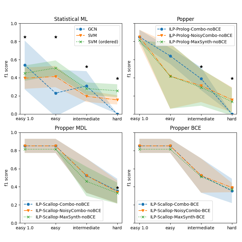
## Line Charts: Performance Comparison of Different Models ### Overview The image presents four line charts comparing the performance (f1 score) of different models across varying difficulty levels (easy 1.0, easy, intermediate, hard). Each chart represents a different model category: Statistical ML, Popper, Propper MDL, and Propper BCE. The charts display the f1 score on the y-axis and the difficulty level on the x-axis. Shaded regions around the lines indicate uncertainty or variance in the performance. Black stars are placed above certain data points, possibly indicating statistical significance or other important metrics. ### Components/Axes * **Titles:** * Top-left: Statistical ML * Top-right: Popper * Bottom-left: Propper MDL * Bottom-right: Propper BCE * **Y-axis:** f1 score, ranging from 0.0 to 1.0 in increments of 0.2. * **X-axis:** Difficulty levels: easy 1.0, easy, intermediate, hard. * **Legends:** Located in the top-right corner of each chart. * **Statistical ML:** * Blue line with circle markers: GCN * Orange line with triangle markers: SVM * Green line with cross markers: SVM (ordered) * **Popper:** * Blue line with circle markers: ILP-Prolog-Combo-noBCE * Orange line with triangle markers: ILP-Prolog-NoisyCombo-noBCE * Green line with cross markers: ILP-Prolog-MaxSynth-noBCE * **Propper MDL:** * Blue line with circle markers: ILP-Scallop-Combo-noBCE * Orange line with triangle markers: ILP-Scallop-NoisyCombo-noBCE * Green line with cross markers: ILP-Scallop-MaxSynth-noBCE * **Propper BCE:** * Blue line with circle markers: ILP-Scallop-Combo-BCE * Orange line with triangle markers: ILP-Scallop-NoisyCombo-BCE * Green line with cross markers: ILP-Scallop-MaxSynth-BCE ### Detailed Analysis **1. Statistical ML** * **GCN (Blue):** Starts at approximately 0.55 f1 score at "easy 1.0", decreases to around 0.23 at "easy", increases to approximately 0.32 at "intermediate", and decreases again to about 0.20 at "hard". * **SVM (Orange):** Starts at approximately 0.45 f1 score at "easy 1.0", decreases to around 0.20 at "easy", increases to approximately 0.25 at "intermediate", and remains around 0.20 at "hard". * **SVM (ordered) (Green):** Starts at approximately 0.45 f1 score at "easy 1.0", increases to around 0.50 at "easy", decreases to approximately 0.30 at "intermediate", and decreases again to about 0.25 at "hard". **2. Popper** * **ILP-Prolog-Combo-noBCE (Blue):** Starts at approximately 0.90 f1 score at "easy 1.0", decreases to around 0.60 at "easy", decreases to approximately 0.40 at "intermediate", and decreases again to about 0.15 at "hard". * **ILP-Prolog-NoisyCombo-noBCE (Orange):** Starts at approximately 0.85 f1 score at "easy 1.0", decreases to around 0.40 at "easy", decreases to approximately 0.30 at "intermediate", and decreases again to about 0.15 at "hard". * **ILP-Prolog-MaxSynth-noBCE (Green):** Starts at approximately 0.85 f1 score at "easy 1.0", decreases to around 0.50 at "easy", decreases to approximately 0.25 at "intermediate", and decreases again to about 0.15 at "hard". **3. Propper MDL** * **ILP-Scallop-Combo-noBCE (Blue):** Starts at approximately 0.85 f1 score at "easy 1.0", remains around 0.80 at "easy", decreases to approximately 0.50 at "intermediate", and decreases again to about 0.35 at "hard". * **ILP-Scallop-NoisyCombo-noBCE (Orange):** Starts at approximately 0.85 f1 score at "easy 1.0", remains around 0.80 at "easy", decreases to approximately 0.50 at "intermediate", and decreases again to about 0.35 at "hard". * **ILP-Scallop-MaxSynth-noBCE (Green):** Starts at approximately 0.85 f1 score at "easy 1.0", remains around 0.80 at "easy", decreases to approximately 0.50 at "intermediate", and decreases again to about 0.35 at "hard". **4. Propper BCE** * **ILP-Scallop-Combo-BCE (Blue):** Starts at approximately 0.85 f1 score at "easy 1.0", remains around 0.80 at "easy", decreases to approximately 0.50 at "intermediate", and decreases again to about 0.35 at "hard". * **ILP-Scallop-NoisyCombo-BCE (Orange):** Starts at approximately 0.85 f1 score at "easy 1.0", remains around 0.80 at "easy", decreases to approximately 0.50 at "intermediate", and decreases again to about 0.35 at "hard". * **ILP-Scallop-MaxSynth-BCE (Green):** Starts at approximately 0.85 f1 score at "easy 1.0", remains around 0.80 at "easy", decreases to approximately 0.50 at "intermediate", and decreases again to about 0.35 at "hard". ### Key Observations * In the Statistical ML chart, the GCN model shows a more fluctuating performance across difficulty levels compared to the SVM models. * In the Popper chart, all three models exhibit a significant decrease in performance as the difficulty level increases. * In the Propper MDL and Propper BCE charts, all three models show similar performance trends, with a plateau at easier difficulty levels followed by a decrease as difficulty increases. * The black stars appear to be placed at points where the f1 score is relatively high or where there might be a significant change in performance. ### Interpretation The charts provide a comparative analysis of different models' performance across varying difficulty levels. The general trend observed is that as the difficulty level increases, the f1 score tends to decrease, indicating a decline in performance. The shaded regions represent the uncertainty or variance in the model's performance, which could be due to factors such as data variability or model instability. The black stars highlight specific data points that may be of particular interest, such as peak performance or significant changes in performance. The choice of model depends on the specific application and the desired trade-off between performance and difficulty level. For example, in the Statistical ML category, the SVM (ordered) model might be preferred for its relatively stable performance across different difficulty levels, while in the Popper category, the ILP-Prolog-Combo-noBCE model might be chosen for its higher initial performance at easier difficulty levels. The Propper MDL and Propper BCE models show similar performance trends, suggesting that the choice between them might depend on other factors such as computational cost or ease of implementation.