## Chart/Diagram Type: Neuromorphic Computing Performance Analysis
### Overview
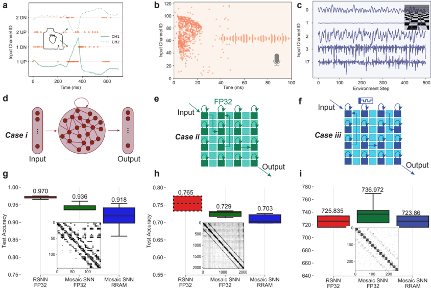
The image presents a series of plots and diagrams evaluating the performance of different neuromorphic computing architectures (RSNN FP32, Mosaic SNN FP32, and RRAM) on a spiking neural network task. It includes time-series data of input signals, schematic representations of network architectures, and box plots comparing test accuracy and inference speed.
### Components/Axes
* **a:** Time-series plot of two input channels (CH1 and CH2) over time (0-600 ms). The y-axis represents Input Channel ID (1 UP, 1 DN, 2 UP, 2 DN).
* **b:** Scatter plot of Input Channel ID (0-120) versus Time (0-100 ms). A microphone icon is present.
* **c:** Time-series plot of Input Channel ID (1-17) versus Environment Step (0-500).
* **d:** Schematic diagram illustrating Case i: a fully connected network with Input and Output layers.
* **e:** Schematic diagram illustrating Case ii: a network with a FP32 layer between Input and Output.
* **f:** Schematic diagram illustrating Case iii: a network with a FP32 layer and a processing unit between Input and Output.
* **g:** Box plot comparing Test Accuracy (0.75-1.00) for RSNN FP32, Mosaic SNN FP32, and RRAM. The x-axis represents the architecture.
* **h:** Box plot comparing Test Accuracy (0.55-0.80) for RSNN FP32, Mosaic SNN FP32, and RRAM. The x-axis represents the architecture. Inset plot shows a zoomed-in view of the data.
* **i:** Box plot comparing inference speed (640-780) for RSNN FP32, Mosaic SNN FP32, and RRAM. The x-axis represents the architecture. Inset plot shows a zoomed-in view of the data.
### Detailed Analysis or Content Details
**a:** The plot shows two fluctuating signals (CH1 and CH2). CH1 appears to have a higher frequency and amplitude than CH2. The signals are approximately periodic, with peaks and troughs occurring roughly every 100-200 ms.
**b:** The scatter plot shows a dense cluster of points, indicating a high frequency of activity in the lower Input Channel IDs (around 20-40) during the initial time period (0-20 ms). The density of points decreases over time, and the distribution becomes more spread out.
**c:** The plot shows fluctuating signals across multiple Input Channels. The signals appear noisy and irregular.
**d:** Case i depicts a network with a circular Input layer connected to an elliptical Output layer. The connections appear to be fully connected.
**e:** Case ii shows a network with an Input layer connected to a square FP32 layer, which is then connected to an Output layer.
**f:** Case iii shows a network with an Input layer connected to a square FP32 layer, which is then connected to a processing unit (represented by a square with a symbol), and finally to an Output layer.
**g:** RSNN FP32 has the highest median Test Accuracy at approximately 0.970, with a range from approximately 0.95 to 0.99. Mosaic SNN FP32 has a median Test Accuracy of approximately 0.936, with a range from approximately 0.91 to 0.96. RRAM has a median Test Accuracy of approximately 0.918, with a range from approximately 0.89 to 0.94.
**h:** RSNN FP32 has a median Test Accuracy of approximately 0.765, with a range from approximately 0.73 to 0.79. Mosaic SNN FP32 has a median Test Accuracy of approximately 0.729, with a range from approximately 0.69 to 0.76. RRAM has a median Test Accuracy of approximately 0.703, with a range from approximately 0.67 to 0.73.
**i:** RSNN FP32 has a median inference speed of approximately 736.972, with a range from approximately 725 to 750. Mosaic SNN FP32 has a median inference speed of approximately 723.86, with a range from approximately 700 to 740. RRAM has a median inference speed of approximately 725.835, with a range from approximately 680 to 760.
### Key Observations
* RSNN FP32 consistently outperforms Mosaic SNN FP32 and RRAM in terms of Test Accuracy in both box plots (g and h).
* RSNN FP32 also exhibits the highest inference speed, although the differences between the architectures are relatively small.
* The input signals (a, b, c) exhibit varying degrees of complexity and noise.
* The network architectures (d, e, f) demonstrate a progression from a simple fully connected network to more complex architectures incorporating FP32 layers and processing units.
### Interpretation
The data suggests that RSNN FP32 is the most effective architecture for the given spiking neural network task, achieving the highest Test Accuracy and inference speed. The inclusion of FP32 layers (as seen in Cases ii and iii) appears to improve performance compared to the fully connected network (Case i). The varying input signals (a, b, c) likely represent different types of sensory data or environmental conditions, and the network's ability to process these signals effectively is crucial for its overall performance. The box plots (g, h, i) provide a clear visualization of the performance differences between the architectures, highlighting the advantages of RSNN FP32. The inset plots in h and i provide a more detailed view of the data, revealing the distribution of values and potential outliers. The microphone icon in plot b suggests that the input data may be related to audio signals. The overall study aims to evaluate the trade-offs between accuracy and efficiency in different neuromorphic computing architectures.