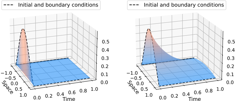
\n ## 3D Surface Plots: Initial and Boundary Conditions ### Overview The image presents two 3D surface plots, likely representing the evolution of a function over time and space. Both plots share a similar structure and visual characteristics, suggesting they depict different stages or conditions of the same underlying phenomenon. The plots visualize a function of two variables, "Time" and "Space", with the surface height representing the function's value. ### Components/Axes Both plots share the following components: * **X-axis:** Labeled "Time", ranging from approximately 0.0 to 1.0. * **Y-axis:** Labeled "Space", ranging from approximately -1.0 to 1.0. * **Z-axis:** Implied, representing the function's value, ranging from approximately 0.0 to 0.5. * **Surface 1 (Orange/Red):** A triangular shaped surface, peaking at Time = 0.0 and Space = 0.0. The color transitions from orange to red. * **Surface 2 (Blue):** A rectangular surface, positioned towards the right of the plot, extending from Time = approximately 0.4 to 1.0 and Space = approximately -1.0 to 1.0. The color is a shade of blue. * **Title:** "--- Initial and boundary conditions ---" positioned at the top of each plot. * **Grid:** A visible grid is present on the base plane of each plot, aiding in visualization. ### Detailed Analysis or Content Details **Plot 1 (Left):** * The orange/red surface is sharply peaked at Time = 0.0 and Space = 0.0, with a value of approximately 0.5. * The blue surface is relatively small, starting at Time = approximately 0.4 and extending to Time = 1.0. Its height is approximately 0.1 to 0.2. * The transition between the orange/red and blue surfaces appears abrupt. **Plot 2 (Right):** * The orange/red surface is similar to Plot 1, peaking at Time = 0.0 and Space = 0.0, with a value of approximately 0.5. * The blue surface is larger than in Plot 1, starting at Time = approximately 0.2 and extending to Time = 1.0. Its height is approximately 0.2 to 0.3. * The transition between the orange/red and blue surfaces appears smoother than in Plot 1. ### Key Observations * Both plots show an initial peak (orange/red surface) followed by the emergence of a rectangular region (blue surface). * The blue surface grows in size over time, as evidenced by the comparison between Plot 1 and Plot 2. * The shape of the orange/red surface remains consistent between the two plots. * The transition between the two surfaces changes from abrupt (Plot 1) to smoother (Plot 2). ### Interpretation The plots likely represent the propagation of a wave or disturbance over time and space. The initial peak (orange/red) could represent the initial condition or source of the disturbance. The blue surface could represent the wave as it propagates and spreads out over time. The difference between the two plots suggests a change in the system's behavior over time. The smoother transition in Plot 2 could indicate that the wave is becoming more stable or that the system is reaching a steady state. The growth of the blue surface indicates that the wave is expanding and covering a larger area. The "Initial and boundary conditions" title suggests that these plots are the result of a simulation or model that is initialized with specific conditions. The plots could be used to visualize the evolution of the system under these conditions. The plots do not provide specific numerical data beyond the axis ranges, but they offer a qualitative understanding of the system's behavior. Further analysis would require access to the underlying data or model.