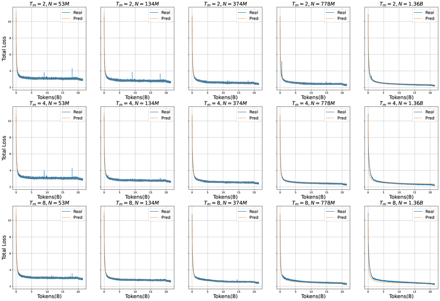
## Line Graphs: Total Loss vs Tokens(B) Across Model Configurations ### Overview The image contains a 3x5 grid of line graphs comparing "Real" and "Predicted" total loss values across different model configurations. Each graph represents a unique combination of training steps (`T_m`) and model size (`N`), with parameters ranging from `T_m = 2, 4, 8` and `N = 53M, 134M, 374M, 778M, 1.36B`. The graphs show how total loss evolves as the number of processed tokens (B) increases during training. --- ### Components/Axes - **X-axis**: "Tokens(B)" (number of processed tokens in billions), scaled from 0 to 20. - **Y-axis**: "Total Loss" (logarithmic scale), ranging from 0 to 10. - **Legend**: Located in the top-right corner of each graph, with: - Solid blue line: "Real" (actual loss values) - Dashed orange line: "Pred" (predicted loss values) - **Graph Titles**: Positioned at the top of each graph, formatted as `T_m = [value], N = [value]` (e.g., `T_m = 2, N = 53M`). --- ### Detailed Analysis #### Trends Across All Graphs 1. **Initial Drop**: Both "Real" and "Pred" lines exhibit a sharp decline in total loss during the first 5–10 tokens(B), indicating rapid improvement in model performance early in training. 2. **Stabilization**: After the initial drop, both lines plateau, showing minimal change in total loss for the remaining tokens(B). The "Pred" line closely tracks the "Real" line, suggesting accurate predictive modeling. 3. **Parameter Impact**: - **Training Steps (`T_m`)**: Higher `T_m` values (e.g., 8 vs. 2) show slightly smoother convergence but no drastic differences in final loss values. - **Model Size (`N`)**: Larger models (e.g., 778M vs. 53M) achieve lower final loss values, indicating better generalization with increased capacity. #### Notable Outliers - In the `T_m = 2, N = 778M` graph, the "Pred" line shows a minor spike (~0.5 loss units) at ~15 tokens(B), but it quickly recovers and aligns with the "Real" line. --- ### Interpretation 1. **Model Performance**: The convergence of "Real" and "Pred" lines across all configurations demonstrates that the predictive model accurately estimates training dynamics, even for large-scale models (up to 1.36B parameters). 2. **Scalability**: Larger models (`N = 778M, 1.36B`) achieve lower final loss values, suggesting that increased model size improves training efficiency and final performance. 3. **Training Dynamics**: The rapid initial drop in loss highlights the importance of early training phases, while the plateau phase indicates diminishing returns after a certain token threshold (~10–15 tokens(B)). --- ### Key Observations - All graphs follow a consistent pattern: sharp initial decline followed by stabilization. - Predictive accuracy ("Pred" vs. "Real") is highest in the early stages of training, with minor deviations later. - Model size (`N`) has a more significant impact on final loss than training steps (`T_m`). --- ### Technical Notes - **Logarithmic Y-axis**: The y-axis uses a logarithmic scale, which emphasizes relative changes in loss during the early, steep decline phase. - **Parameter Ranges**: The `N` values span 3 orders of magnitude (53M to 1.36B), while `T_m` ranges from 2 to 8 steps. - **Legend Consistency**: The solid blue ("Real") and dashed orange ("Pred") lines are consistently placed across all graphs, ensuring visual coherence. --- ### Language and Localization - **Primary Language**: English (all axis labels, legends, and titles are in English). - **No Non-English Text**: No additional languages or annotations are present. --- ### Final Notes This visualization effectively demonstrates the relationship between model configuration (size and training steps) and training dynamics. The alignment of "Real" and "Pred" lines across diverse configurations validates the predictive model's robustness, while the parameter-specific trends provide actionable insights for optimizing training efficiency.