## Scatter Plot and Traveling Salesman Path
### Overview
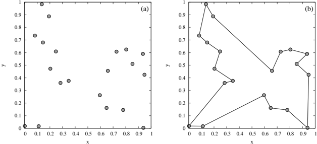
The image presents two scatter plots side-by-side. The left plot, labeled "(a)", shows a random distribution of points. The right plot, labeled "(b)", displays the same points connected by lines, forming a path that appears to minimize the total distance traveled between them, resembling a solution to the Traveling Salesman Problem (TSP).
### Components/Axes
Both plots share the same axes:
* **x-axis:** Labeled "x", ranges from 0 to 1 in increments of 0.1.
* **y-axis:** Labeled "y", ranges from 0 to 1 in increments of 0.1.
* **Data Points:** Represented by gray circles.
* **Path (Plot b):** Represented by black lines connecting the data points.
### Detailed Analysis
**Plot (a): Scatter Plot**
The points are scattered relatively randomly across the plot area. Here are approximate coordinates for some of the points:
* (0, 0): One point
* (0.1, 0): One point
* (0.1, 0.73): One point
* (0.2, 0.9): One point
* (0.2, 0.6): One point
* (0.3, 0.4): One point
* (0.35, 0.35): One point
* (0.4, 0.4): One point
* (0.6, 0.25): One point
* (0.7, 0.15): One point
* (0.75, 0.6): One point
* (0.8, 0.65): One point
* (0.8, 0.5): One point
* (0.9, 0.6): One point
* (0.9, 0.4): One point
**Plot (b): Traveling Salesman Path**
The points from plot (a) are connected by a path. The path starts at approximately (0,0) and visits each point once before returning to the starting point. The path appears to be a reasonable approximation of the shortest possible route connecting all the points.
Here's a breakdown of the path's segments and approximate coordinates of the points it connects:
1. (0, 0) to (0.1, 0)
2. (0.1, 0) to (0.1, 0.73)
3. (0.1, 0.73) to (0.2, 0.9)
4. (0.2, 0.9) to (0.2, 0.6)
5. (0.2, 0.6) to (0.35, 0.35)
6. (0.35, 0.35) to (0.4, 0.4)
7. (0.4, 0.4) to (0.6, 0.25)
8. (0.6, 0.25) to (0.7, 0.15)
9. (0.7, 0.15) to (0.9, 0.4)
10. (0.9, 0.4) to (0.9, 0)
11. (0.9, 0) to (0.9, 0.6)
12. (0.9, 0.6) to (0.8, 0.65)
13. (0.8, 0.65) to (0.75, 0.6)
14. (0.75, 0.6) to (0.8, 0.5)
15. (0.8, 0.5) to (0.2, 0.6)
16. (0.2, 0.6) to (0, 0)
### Key Observations
* Plot (a) shows a random distribution of points.
* Plot (b) demonstrates a possible solution to the Traveling Salesman Problem for the points in plot (a).
* The path in plot (b) attempts to minimize the total distance traveled.
### Interpretation
The image illustrates the Traveling Salesman Problem (TSP), a classic optimization problem. Plot (a) represents the set of locations (cities) that need to be visited. Plot (b) shows a possible solution to the TSP, where a path is constructed that visits each location exactly once and returns to the starting point, while attempting to minimize the total distance traveled. The TSP is NP-hard, meaning that finding the optimal solution becomes computationally expensive as the number of locations increases. The path shown in plot (b) is likely a heuristic solution, meaning it's a good approximation but not necessarily the absolute shortest path.