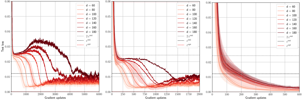
## Test Loss vs. Gradient Updates for Varying Dimensions ### Overview The image presents three line charts comparing the test loss against gradient updates for different dimensions (d = 60, 80, 100, 120, 140, 160, 180). Each chart represents a different scaling of the x-axis (Gradient updates), showing the initial behavior in more detail. The charts also include horizontal lines representing `2 * epsilon_uni`, `epsilon_uni`, and `epsilon_opt`. The lines are color-coded according to the legend in the top-right of each chart. ### Components/Axes * **X-axis (Horizontal):** Gradient updates. The scale varies across the three charts. * Left Chart: 0 to 6000 * Middle Chart: 0 to 2000 * Right Chart: 0 to 600 * **Y-axis (Vertical):** Test loss, ranging from 0.00 to 0.06 in all three charts. * **Legend (Top-Right):** * d = 60 (lightest red) * d = 80 (lighter red) * d = 100 (mid-tone red) * d = 120 (slightly darker red) * d = 140 (darker red) * d = 160 (dark red) * d = 180 (darkest red/brown) * 2 * epsilon^uni (light gray dashed line) * epsilon^uni (dark gray dashed line) * epsilon^opt (red dashed line) ### Detailed Analysis **Left Chart (Gradient Updates: 0 to 6000):** * **d = 60 (lightest red):** Starts at approximately 0.022, decreases to approximately 0.005 around 2000 gradient updates, then fluctuates around that value. * **d = 80 (lighter red):** Starts at approximately 0.023, decreases to approximately 0.007 around 2500 gradient updates, then fluctuates. * **d = 100 (mid-tone red):** Starts at approximately 0.024, decreases to approximately 0.008 around 3000 gradient updates, then fluctuates. * **d = 120 (slightly darker red):** Starts at approximately 0.025, decreases to approximately 0.01 around 3500 gradient updates, then fluctuates. * **d = 140 (darker red):** Starts at approximately 0.026, decreases to approximately 0.012 around 4000 gradient updates, then fluctuates. * **d = 160 (dark red):** Starts at approximately 0.027, increases to approximately 0.032 around 2000 gradient updates, then decreases to approximately 0.013 around 4500 gradient updates, then fluctuates. * **d = 180 (darkest red/brown):** Starts at approximately 0.028, increases to approximately 0.035 around 2500 gradient updates, then decreases to approximately 0.014 around 5000 gradient updates, then fluctuates. * **2 * epsilon^uni (light gray dashed line):** Horizontal line at approximately 0.023. * **epsilon^uni (dark gray dashed line):** Horizontal line at approximately 0.012. * **epsilon^opt (red dashed line):** Horizontal line at approximately 0.025. **Middle Chart (Gradient Updates: 0 to 2000):** * **d = 60 (lightest red):** Starts at approximately 0.022, rapidly decreases to approximately 0.005 within the first 500 gradient updates. * **d = 80 (lighter red):** Starts at approximately 0.023, rapidly decreases to approximately 0.007 within the first 750 gradient updates. * **d = 100 (mid-tone red):** Starts at approximately 0.024, rapidly decreases to approximately 0.008 within the first 1000 gradient updates. * **d = 120 (slightly darker red):** Starts at approximately 0.025, decreases to approximately 0.01 around 1250 gradient updates. * **d = 140 (darker red):** Starts at approximately 0.026, decreases to approximately 0.012 around 1500 gradient updates. * **d = 160 (dark red):** Starts at approximately 0.027, increases to approximately 0.022 around 500 gradient updates, then decreases to approximately 0.013 around 1750 gradient updates. * **d = 180 (darkest red/brown):** Starts at approximately 0.028, increases to approximately 0.023 around 750 gradient updates, then decreases to approximately 0.014 around 2000 gradient updates. * **2 * epsilon^uni (light gray dashed line):** Horizontal line at approximately 0.023. * **epsilon^uni (dark gray dashed line):** Horizontal line at approximately 0.012. * **epsilon^opt (red dashed line):** Horizontal line at approximately 0.025. **Right Chart (Gradient Updates: 0 to 600):** * **d = 60 (lightest red):** Starts at approximately 0.06, rapidly decreases to approximately 0.015 within the first 100 gradient updates, then continues to decrease to approximately 0.005 by 600 gradient updates. * **d = 80 (lighter red):** Starts at approximately 0.06, rapidly decreases to approximately 0.017 within the first 100 gradient updates, then continues to decrease to approximately 0.007 by 600 gradient updates. * **d = 100 (mid-tone red):** Starts at approximately 0.06, rapidly decreases to approximately 0.018 within the first 100 gradient updates, then continues to decrease to approximately 0.008 by 600 gradient updates. * **d = 120 (slightly darker red):** Starts at approximately 0.06, rapidly decreases to approximately 0.019 within the first 100 gradient updates, then continues to decrease to approximately 0.01 by 600 gradient updates. * **d = 140 (darker red):** Starts at approximately 0.06, rapidly decreases to approximately 0.02 within the first 100 gradient updates, then continues to decrease to approximately 0.012 by 600 gradient updates. * **d = 160 (dark red):** Starts at approximately 0.06, rapidly decreases to approximately 0.021 within the first 100 gradient updates, then continues to decrease to approximately 0.013 by 600 gradient updates. * **d = 180 (darkest red/brown):** Starts at approximately 0.06, rapidly decreases to approximately 0.022 within the first 100 gradient updates, then continues to decrease to approximately 0.014 by 600 gradient updates. * **2 * epsilon^uni (light gray dashed line):** Horizontal line at approximately 0.023. * **epsilon^uni (dark gray dashed line):** Horizontal line at approximately 0.012. * **epsilon^opt (red dashed line):** Horizontal line at approximately 0.025. ### Key Observations * For smaller dimensions (d = 60, 80, 100), the test loss decreases rapidly and stabilizes at a low value. * For larger dimensions (d = 160, 180), the test loss initially increases before decreasing, and the final loss is higher than for smaller dimensions. * The rate of decrease in test loss is highest in the initial gradient updates (as seen in the right chart). * The horizontal lines representing `2 * epsilon_uni`, `epsilon_uni`, and `epsilon_opt` provide reference points for evaluating the test loss. ### Interpretation The charts suggest that there is an optimal dimension for the model. Smaller dimensions lead to faster convergence and lower final test loss. However, larger dimensions may initially struggle to decrease the loss, and they may also converge to a higher final loss. This could be due to overfitting or other issues related to model complexity. The values of `epsilon_uni` and `epsilon_opt` seem to represent theoretical bounds or target values for the test loss, and the performance of different dimensions can be evaluated relative to these bounds. The initial increase in test loss for larger dimensions suggests that the model may be initially exploring suboptimal regions of the parameter space before finding a better solution.