# Technical Data Extraction: Spatial Distribution and Current Flow in Nanostructures
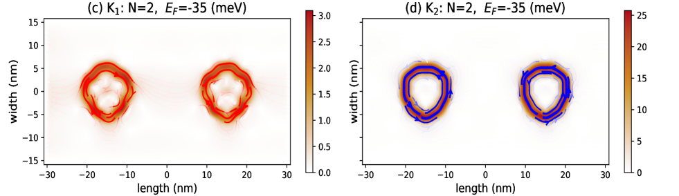
This document provides a detailed technical extraction of the data presented in the provided image, which consists of two side-by-side heatmaps with overlaid vector flow lines, likely representing physical properties (such as local density of states or current density) in a nanostructure.
## 1. Global Metadata and Parameters
The image contains two panels, labeled (c) and (d). Both panels share common physical parameters:
* **N (Number of units/particles):** 2
* **$E_F$ (Fermi Energy):** -35 (meV)
* **X-Axis (Length):** Measured in nanometers (nm), ranging from -30 to 30.
* **Y-Axis (Width):** Measured in nanometers (nm), ranging from -15 to 15.
---
## 2. Panel (c) Analysis: $K_1$ Distribution
### Header Information
* **Label:** (c) $K_1$: N=2, $E_F$=-35 (meV)
### Spatial Grounding and Components
* **Main Chart:** Displays two distinct circular/annular regions of intensity centered at approximately $x = -15$ nm and $x = +15$ nm along the $y = 0$ axis.
* **Color Scale (Right Side):** A vertical gradient bar ranging from **0.0 to 3.0**. The color transitions from white (0.0) to light orange, then to deep red/brown (3.0).
* **Flow Lines:** Overlaid on the intensity regions are bright red streamlines with arrowheads indicating direction.
### Data Trends and Observations
* **Intensity Distribution:** The intensity is concentrated in two ring-like structures. The peak intensity (darkest red, ~3.0 on the scale) forms a jagged, hexagonal-like perimeter around a lower-intensity center.
* **Current/Flow Direction:** The red streamlines indicate a **clockwise** circulation pattern around the center of each of the two structures.
* **Interaction:** There is very little "bleeding" or interaction between the two structures; the region at $x = 0$ shows near-zero intensity (white).
---
## 3. Panel (d) Analysis: $K_2$ Distribution
### Header Information
* **Label:** (d) $K_2$: N=2, $E_F$=-35 (meV)
### Spatial Grounding and Components
* **Main Chart:** Similar to panel (c), it displays two distinct annular regions centered at $x = -15$ nm and $x = +15$ nm.
* **Color Scale (Right Side):** A vertical gradient bar ranging from **0 to 25**. Note that the magnitude is significantly higher (nearly 8x) than in panel (c). The color transitions from white (0) to orange-brown (25).
* **Flow Lines:** Overlaid on the intensity regions are dark blue streamlines with arrowheads.
### Data Trends and Observations
* **Intensity Distribution:** The spatial footprint is nearly identical to panel (c), but the numerical values are much higher. The highest intensity (darkest brown, ~25) is concentrated in the outer ring of the structures.
* **Current/Flow Direction:** The blue streamlines indicate a **counter-clockwise** circulation pattern. This is the inverse of the flow direction observed in panel (c).
* **Symmetry:** The two structures (left and right) appear to be mirror images or identical copies of each other in terms of flow and intensity.
---
## 4. Comparative Summary Table
| Feature | Panel (c) - $K_1$ | Panel (d) - $K_2$ |
| :--- | :--- | :--- |
| **Max Scale Value** | 3.0 | 25 |
| **Flow Line Color** | Red | Blue |
| **Flow Direction** | Clockwise | Counter-clockwise |
| **Center Positions** | $x \approx \pm 15$ nm, $y \approx 0$ nm | $x \approx \pm 15$ nm, $y \approx 0$ nm |
| **Structure Shape** | Annular / Hexagonal Ring | Annular / Hexagonal Ring |
## 5. Conclusion
The data represents two distinct states or components ($K_1$ and $K_2$) of a system with two localized centers. While the spatial geometry of the intensity is consistent across both panels, $K_2$ exhibits a much higher magnitude and an opposite rotational flow compared to $K_1$. This likely represents valley-polarized or spin-polarized currents where $K_1$ and $K_2$ refer to different momentum space valleys.