\n
## Charts: Pulse Amplitude vs. Time for Different CIM Configurations
### Overview
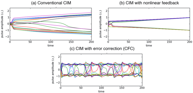
The image presents three separate line charts, labeled (a) Conventional CIM, (b) CIM with nonlinear feedback, and (c) CIM with error correction (CFC). Each chart plots pulse amplitude (x<sub>r</sub>) against time, ranging from 0 to 200. The charts visually compare the behavior of pulse amplitudes under different CIM (Computation In Memory) configurations.
### Components/Axes
* **X-axis:** Time (ranging from 0 to 200, units not specified).
* **Y-axis:** Pulse Amplitude (x<sub>r</sub>), ranging from approximately -2 to 2, units not specified.
* **Chart (a):** Conventional CIM. Multiple lines representing individual pulse amplitudes.
* **Chart (b):** CIM with nonlinear feedback. Multiple lines representing individual pulse amplitudes.
* **Chart (c):** CIM with error correction (CFC). Multiple lines representing individual pulse amplitudes.
* **No Legend:** There is no explicit legend provided for the line colors in any of the charts. Each chart contains multiple lines, each representing a different pulse amplitude, but their specific identities are not labeled.
### Detailed Analysis or Content Details
**Chart (a): Conventional CIM**
* **Trend:** The lines generally converge towards the top of the chart initially, then diverge and spread out over time. Some lines exhibit a downward trend, while others remain relatively stable or slightly increase.
* **Data Points (approximate):**
* At time = 0, most lines start around a pulse amplitude of 1.5 to 2.
* At time = 50, pulse amplitudes range from approximately -0.5 to 1.8.
* At time = 100, pulse amplitudes range from approximately -1.2 to 1.5.
* At time = 150, pulse amplitudes range from approximately -1.8 to 1.2.
* At time = 200, pulse amplitudes range from approximately -1.5 to 1.7.
* There is a line that starts at approximately 1.8 and decreases to approximately -1.5 by time = 150.
**Chart (b): CIM with nonlinear feedback**
* **Trend:** The lines converge rapidly towards a single value near the top of the chart and remain relatively stable over time.
* **Data Points (approximate):**
* At time = 0, lines start between approximately -1 and 1.5.
* At time = 50, lines are clustered around a pulse amplitude of approximately 0.8 to 1.2.
* At time = 100, lines are clustered around a pulse amplitude of approximately 0.8 to 1.2.
* At time = 150, lines are clustered around a pulse amplitude of approximately 0.8 to 1.2.
* At time = 200, lines are clustered around a pulse amplitude of approximately 0.8 to 1.2.
* There is a line that starts at approximately -1 and converges to approximately 0.8 by time = 50.
**Chart (c): CIM with error correction (CFC)**
* **Trend:** The lines oscillate rapidly and consistently around a central value, exhibiting a periodic behavior.
* **Data Points (approximate):**
* At time = 0, lines range from approximately -1.5 to 1.5.
* At time = 50, lines range from approximately -1.5 to 1.5.
* At time = 100, lines range from approximately -1.5 to 1.5.
* At time = 150, lines range from approximately -1.5 to 1.5.
* At time = 200, lines range from approximately -1.5 to 1.5.
* The oscillations appear to have a consistent amplitude and frequency throughout the duration of the chart.
### Key Observations
* The Conventional CIM (a) exhibits the most significant divergence in pulse amplitudes over time, indicating instability or varying behavior.
* The CIM with nonlinear feedback (b) demonstrates the most stable behavior, with pulse amplitudes converging to a consistent value.
* The CIM with error correction (CFC) (c) shows a consistent oscillatory behavior, suggesting a controlled and periodic response.
* The lack of a legend makes it impossible to identify specific pulse amplitudes or their corresponding lines.
### Interpretation
The data suggests that the implementation of nonlinear feedback and error correction techniques significantly improves the stability and control of pulse amplitudes in CIM systems. The conventional CIM configuration exhibits a wider range of behaviors, potentially leading to unpredictable results. The nonlinear feedback configuration effectively stabilizes the pulse amplitudes, while the error correction configuration introduces a controlled oscillatory behavior.
The oscillatory behavior in the CFC configuration might be intentional, representing a desired operational characteristic of the system. The convergence in chart (b) suggests a self-regulating mechanism, while the divergence in chart (a) indicates a lack of such control.
The absence of a legend limits the ability to draw more specific conclusions about individual pulse amplitudes. However, the overall trends clearly demonstrate the benefits of incorporating feedback and error correction mechanisms in CIM designs. The charts provide a comparative analysis of different CIM configurations, highlighting their respective strengths and weaknesses in terms of pulse amplitude stability and control.