## Charts: Scaling Laws for Neural Network Training
### Overview
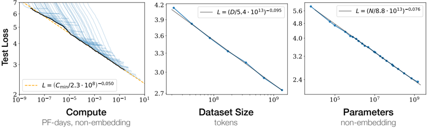
The image presents three charts illustrating scaling laws for neural network training. Each chart explores the relationship between "Test Loss" and a different factor: "Compute", "Dataset Size", and "Parameters". The charts show how test loss decreases as these factors increase, with each chart also including a fitted power law curve.
### Components/Axes
* **Common Y-axis:** "Test Loss" ranging from approximately 2 to 7.
* **Chart 1 (Left):**
* X-axis: "Compute" (PF-days, non-embedding) on a logarithmic scale from 10<sup>-6</sup> to 10<sup>1</sup>.
* Data Series 1 (Blue, faint lines): Multiple individual training runs showing test loss vs. compute.
* Data Series 2 (Orange, bold line): A fitted curve representing the scaling law: L = (C<sub>min</sub>/(2.3 * 10<sup>9</sup>))<sup>-0.050</sup>
* **Chart 2 (Center):**
* X-axis: "Dataset Size" (tokens) on a logarithmic scale from 10<sup>7</sup> to 10<sup>10</sup>.
* Data Series 1 (Blue, bold line): A fitted curve representing the scaling law: L = (D/(5.4 * 10<sup>43</sup>))<sup>-0.095</sup>
* **Chart 3 (Right):**
* X-axis: "Parameters" (non-embedding) on a logarithmic scale from 10<sup>5</sup> to 10<sup>9</sup>.
* Data Series 1 (Blue, bold line): A fitted curve representing the scaling law: L = (N/(8.8 * 10<sup>13</sup>))<sup>-0.076</sup>
### Detailed Analysis or Content Details
* **Chart 1 (Compute):** The blue lines represent individual training runs, showing a wide range of test loss values for a given compute level. The orange line, representing the scaling law, slopes downward, indicating that as compute increases, test loss decreases.
* At Compute = 10<sup>-6</sup>, Test Loss ≈ 6.5
* At Compute = 10<sup>-1</sup>, Test Loss ≈ 3.0
* At Compute = 10<sup>1</sup>, Test Loss ≈ 2.2
* **Chart 2 (Dataset Size):** The blue line slopes downward, indicating that as dataset size increases, test loss decreases.
* At Dataset Size = 10<sup>7</sup>, Test Loss ≈ 4.2
* At Dataset Size = 10<sup>9</sup>, Test Loss ≈ 2.8
* At Dataset Size = 10<sup>10</sup>, Test Loss ≈ 2.7
* **Chart 3 (Parameters):** The blue line slopes downward, indicating that as the number of parameters increases, test loss decreases.
* At Parameters = 10<sup>5</sup>, Test Loss ≈ 5.6
* At Parameters = 10<sup>7</sup>, Test Loss ≈ 3.5
* At Parameters = 10<sup>9</sup>, Test Loss ≈ 2.5
### Key Observations
* All three charts demonstrate a clear inverse relationship between the input factor (Compute, Dataset Size, Parameters) and Test Loss.
* The scaling laws (orange/blue lines) provide a general trend, but individual training runs (blue lines in Chart 1) exhibit significant variance.
* The rate of decrease in test loss appears to diminish as the input factor increases in all three charts.
### Interpretation
These charts illustrate the scaling laws governing the performance of neural networks. They demonstrate that increasing compute, dataset size, and the number of parameters generally leads to lower test loss, and thus improved model performance. The fitted power law curves provide a quantitative relationship between these factors and test loss, allowing for predictions about the performance of models with different configurations. The variance observed in Chart 1 suggests that other factors, beyond compute, also influence model performance. The diminishing returns observed in all charts indicate that there are limits to the benefits of simply scaling up these factors. The specific exponents in the power laws (e.g., -0.050, -0.095, -0.076) quantify the sensitivity of test loss to changes in each factor. These findings are crucial for efficient resource allocation and model design in machine learning.