## Multi-Plot Analysis of Performance Metrics vs. Lambda
### Overview
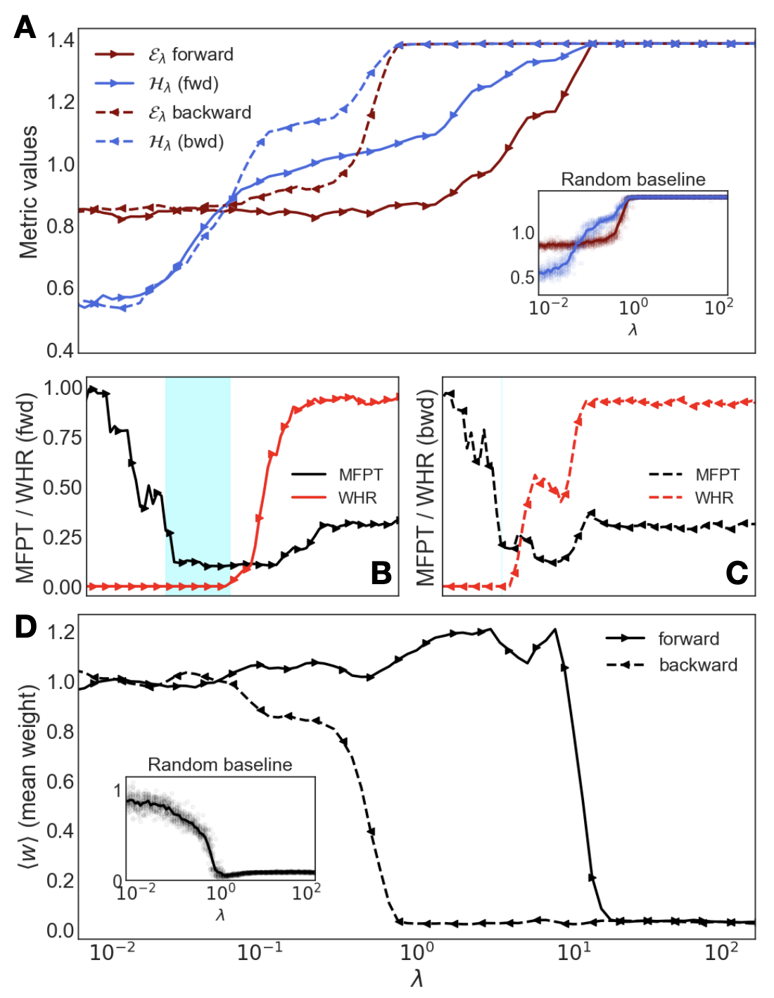
The image presents four plots (A, B, C, and D) and two insets, each displaying different performance metrics as a function of the parameter lambda (λ). The plots explore forward and backward perspectives, and compare metrics like Epsilon (ε), H, MFPT (Mean First Passage Time), and WHR (Weight Histogram Ratio). The insets provide "Random baseline" comparisons for specific metrics.
### Components/Axes
**Plot A:**
* **Title:** (Implied) Performance Metrics vs. Lambda
* **Y-axis:** "Metric values", ranging from 0.4 to 1.4.
* **X-axis:** Lambda (λ), implied to be shared with other plots.
* **Legend (top-left):**
* Red solid line: "ελ forward"
* Blue solid line: "Hλ (fwd)"
* Red dashed line: "ελ backward"
* Blue dashed line: "Hλ (bwd)"
**Plot B:**
* **Title:** MFPT / WHR (fwd) vs. Lambda
* **Y-axis:** "MFPT / WHR (fwd)", ranging from 0.00 to 1.00.
* **X-axis:** Lambda (λ), implied.
* **Legend (center-right):**
* Black solid line: "MFPT"
* Red solid line: "WHR"
* Light blue shaded region spans approximately from λ = 0.02 to λ = 0.07.
**Plot C:**
* **Title:** MFPT / WHR (bwd) vs. Lambda
* **Y-axis:** "MFPT / WHR (bwd)", ranging from 0.00 to 1.00.
* **X-axis:** Lambda (λ), implied.
* **Legend (center-right):**
* Black dashed line: "MFPT"
* Red dashed line: "WHR"
* Light blue shaded region spans approximately from λ = 0.02 to λ = 0.07.
**Plot D:**
* **Title:** (w) (mean weight) vs. Lambda
* **Y-axis:** "(w) (mean weight)", ranging from 0.0 to 1.2.
* **X-axis:** Lambda (λ), ranging from 10^-2 to 10^2 (log scale).
* **Legend (top-right):**
* Black solid line: "forward"
* Black dashed line: "backward"
**Inset Plots:**
* **Plot A Inset:** "Random baseline" comparison for ελ. Y-axis ranges from approximately 0.5 to 1.1. X-axis is Lambda (λ), ranging from 10^-2 to 10^2 (log scale).
* **Plot D Inset:** "Random baseline" comparison for (w). Y-axis ranges from approximately 0 to 1. X-axis is Lambda (λ), ranging from 10^-2 to 10^2 (log scale).
### Detailed Analysis
**Plot A:**
* **ελ forward (red solid line):** Starts at approximately 0.85, remains relatively constant until λ ≈ 0.1, then increases to approximately 1.1 at λ ≈ 1, and continues to increase to approximately 1.4, plateauing around λ = 10.
* **Hλ (fwd) (blue solid line):** Starts at approximately 0.55, increases sharply to approximately 1.2 at λ ≈ 0.1, and then plateaus around 1.4.
* **ελ backward (red dashed line):** Starts at approximately 0.85, remains relatively constant until λ ≈ 0.1, then increases to approximately 1.35, plateauing around λ = 1.
* **Hλ (bwd) (blue dashed line):** Starts at approximately 0.55, increases sharply to approximately 1.1 at λ ≈ 0.1, and then plateaus around 1.4.
**Plot B:**
* **MFPT (black solid line):** Starts at 1.0, decreases sharply to approximately 0.1 at λ ≈ 0.05, then increases to approximately 0.3 at λ ≈ 1, and then decreases again to approximately 0.25.
* **WHR (red solid line):** Starts at approximately 0.0, remains at 0 until λ ≈ 0.07, then increases sharply to approximately 0.95, plateauing around 1.0.
**Plot C:**
* **MFPT (black dashed line):** Starts at approximately 1.0, decreases sharply to approximately 0.1 at λ ≈ 0.05, then increases to approximately 0.3 at λ ≈ 1, and then decreases again to approximately 0.25.
* **WHR (red dashed line):** Starts at approximately 0.0, remains at 0 until λ ≈ 0.07, then increases sharply to approximately 0.95, plateauing around 1.0.
**Plot D:**
* **Forward (black solid line):** Starts at approximately 1.0, remains relatively constant until λ ≈ 5, then decreases sharply to approximately 0.0 at λ ≈ 10, and remains at 0.
* **Backward (black dashed line):** Starts at approximately 1.0, decreases gradually to approximately 0.8 at λ ≈ 1, then decreases sharply to approximately 0.0 at λ ≈ 10, and remains at 0.
**Inset Plots:**
* **Plot A Inset:** The data points are scattered, but the trend shows both forward and backward epsilon values starting around 0.5, increasing to approximately 0.9 around λ = 1, and then plateauing.
* **Plot D Inset:** The data points are scattered, but the trend shows the mean weight starting around 1.0, decreasing to approximately 0.2 around λ = 1, and then plateauing.
### Key Observations
* In Plot A, the forward and backward metrics (ελ and Hλ) converge to similar values as lambda increases.
* In Plots B and C, the MFPT and WHR metrics exhibit inverse relationships, with MFPT decreasing as WHR increases.
* In Plot D, the forward and backward mean weights diverge significantly as lambda increases, with the forward weight dropping sharply to zero.
* The insets show the "Random baseline" performance, providing a reference point for the main plots.
### Interpretation
The plots illustrate the impact of the parameter lambda (λ) on various performance metrics in forward and backward perspectives. The convergence of forward and backward metrics in Plot A suggests that as lambda increases, the system becomes more stable and less sensitive to the direction of analysis. The inverse relationship between MFPT and WHR in Plots B and C indicates a trade-off between the time it takes to reach a certain state (MFPT) and the distribution of weights (WHR). The sharp drop in forward mean weight in Plot D suggests a critical threshold for lambda, beyond which the forward perspective becomes significantly less relevant. The "Random baseline" insets provide a benchmark for evaluating the effectiveness of the system compared to a random scenario. Overall, the data suggests that lambda plays a crucial role in balancing stability, efficiency, and directionality in the system.