## Line Chart with Shaded Regions: Energy Difference vs. β
### Overview
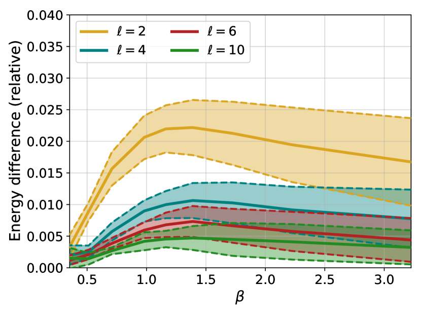
The image is a scientific line chart plotting "Energy difference (relative)" on the y-axis against the parameter "β" on the x-axis. It displays four data series, each corresponding to a different value of "ℓ" (2, 4, 6, 10). Each series is represented by a solid line with a semi-transparent shaded region around it, likely indicating a confidence interval, standard deviation, or range of values.
### Components/Axes
* **Y-Axis:**
* **Label:** "Energy difference (relative)"
* **Scale:** Linear, ranging from 0.000 to 0.040.
* **Major Ticks:** 0.000, 0.005, 0.010, 0.015, 0.020, 0.025, 0.030, 0.035, 0.040.
* **X-Axis:**
* **Label:** "β" (Greek letter beta).
* **Scale:** Linear, ranging from approximately 0.4 to 3.2.
* **Major Ticks:** 0.5, 1.0, 1.5, 2.0, 2.5, 3.0.
* **Legend:**
* **Position:** Top-left corner of the chart area.
* **Entries:**
* `ℓ = 2` (Yellow/Gold solid line)
* `ℓ = 4` (Teal solid line)
* `ℓ = 6` (Red solid line)
* `ℓ = 10` (Green solid line)
* **Note:** The legend only shows the solid line style. The corresponding shaded regions use the same color but with transparency.
### Detailed Analysis
**Trend Verification:** All four data series follow a similar visual trend: they start at a low value near β=0.5, rise to a peak around β=1.5, and then gradually decline as β increases towards 3.0. The magnitude of the energy difference and the width of the shaded region decrease systematically as ℓ increases.
**Data Series Breakdown (Approximate Values):**
1. **ℓ = 2 (Yellow/Gold):**
* **Trend:** Highest curve with the widest shaded region.
* **Key Points:**
* At β ≈ 0.5: y ≈ 0.005
* Peak near β ≈ 1.5: y ≈ 0.022 (solid line), shaded region spans ~0.018 to ~0.026.
* At β ≈ 3.0: y ≈ 0.017 (solid line), shaded region spans ~0.010 to ~0.024.
2. **ℓ = 4 (Teal):**
* **Trend:** Second highest curve.
* **Key Points:**
* At β ≈ 0.5: y ≈ 0.002
* Peak near β ≈ 1.5: y ≈ 0.011 (solid line), shaded region spans ~0.007 to ~0.014.
* At β ≈ 3.0: y ≈ 0.008 (solid line), shaded region spans ~0.005 to ~0.013.
3. **ℓ = 6 (Red):**
* **Trend:** Third highest curve.
* **Key Points:**
* At β ≈ 0.5: y ≈ 0.001
* Peak near β ≈ 1.5: y ≈ 0.008 (solid line), shaded region spans ~0.005 to ~0.010.
* At β ≈ 3.0: y ≈ 0.005 (solid line), shaded region spans ~0.002 to ~0.008.
4. **ℓ = 10 (Green):**
* **Trend:** Lowest curve with the narrowest shaded region.
* **Key Points:**
* At β ≈ 0.5: y ≈ 0.000
* Peak near β ≈ 1.5: y ≈ 0.005 (solid line), shaded region spans ~0.003 to ~0.007.
* At β ≈ 3.0: y ≈ 0.001 (solid line), shaded region spans ~0.000 to ~0.004.
### Key Observations
1. **Systematic Ordering:** There is a clear, monotonic relationship between ℓ and the energy difference. For any given β, the energy difference is highest for ℓ=2 and decreases as ℓ increases (ℓ=2 > ℓ=4 > ℓ=6 > ℓ=10).
2. **Common Peak Location:** All four curves reach their maximum value at approximately the same β value, around 1.5.
3. **Variability Correlates with Magnitude:** The width of the shaded region (uncertainty/variability) is largest for the series with the highest energy difference (ℓ=2) and becomes progressively narrower for series with lower energy differences (ℓ=10).
4. **Convergence at Low β:** All curves appear to converge towards a very low energy difference (near zero) as β approaches 0.4 from the right.
### Interpretation
The chart demonstrates a clear functional relationship where the relative energy difference is a non-monotonic function of β, exhibiting a distinct maximum near β=1.5. This suggests the existence of an optimal β value that maximizes this energy difference metric for the system under study.
The parameter ℓ acts as a scaling or damping factor. Higher ℓ values systematically suppress the energy difference across the entire range of β and also reduce its variability (as indicated by the narrower shaded bands). This could imply that ℓ represents a system size, a coupling strength, or a disorder parameter where increased values lead to more stable or less fluctuating energy states relative to a reference.
The convergence at low β suggests that for small values of this parameter, the system's energy difference becomes negligible and insensitive to the value of ℓ. The most significant differentiation between systems with different ℓ occurs in the intermediate β range (1.0 to 2.0). This type of plot is common in statistical physics or computational materials science, often showing how an energy property (like a formation energy or excitation gap) varies with inverse temperature (β ∝ 1/T) and a system parameter (ℓ).